(3) where cF is a constant. The bounded Frobenius-norm admissible set is defined ..... than 8 hours was recorded from BBC radio 3, which plays mostly classical ...
PARSIMONIOUS DICTIONARY LEARNING Mehrdad Yaghoobi, Thomas Blumensath, Michael E. Davies Institute for Digital Communications, Joint Research Institute for Signal and Image Processing, The University of Edinburgh, EH9 3JL, UK { m.yaghoobi-vaighan, thomas.blumensath, mike.davies}@ed.ac.uk ABSTRACT Sparse modeling of signals has recently received a lot of attention. Often, a linear under-determined generative model for the signals of interest is proposed and a sparsity constraint imposed on the representation. When the generative model is not given, choosing an appropriate generative model is important, so that the given class of signals has approximate sparse representations. In this paper we introduce a new scheme for dictionary learning and impose an additional constraint to reduce the dictionary size. Small dictionaries are desired for coding applications and more likely to “work” with suboptimal algorithms such as Basis Pursuit. Another benefit of small dictionaries is their faster implementation, e.g. a reduced number of multiplication/addition in each matrix vector multiplication, which is the bottleneck in sparse approximation algorithms.
in the sparse approximation of real signals. When the size of the dictionary is unknown, one can start with a oversized dictionary and find the minimum size learnt dictionary. We here introduce a framework for parsimonious dictionary learning. The problem formulation is followed by a practical algorithm to find an approximate solution. We show that the proposed framework gives promising results in dictionary recovery. We then show that the learnt dictionary has advantages over the currently used dictionaries for sparse coding. 2. PARSIMONIOUS DICTIONARY LEARNING FORMULATION Dictionary learning can be formulated as the minimization of a joint objective function based on D and X.
Index Terms— Sparse Approximation, Dictionary Learning, Majorization Method, Sparse Coding 1. INTRODUCTION Let Y = {y (i) : 1 ≤ i ≤ L} be a given set of training samples and X = {x(i) : 1 ≤ i ≤ L} be the corresponding coefficient vectors. Yd×L and XN×L are the matrices generated by using the elements of Y and X as the column vectors, respectively. The dictionary learning problem can be formulated as follows. Given Y, find a “dictionary“ matrix D and a coefficient matrix X, such that the error ǫ = Y−DX is small and X is sparse. This is a challenging problem and researchers from different fields have introduced algorithms to solve it approximately [1–4]. Regardless of the sparsity measure, dictionary learning is a non-convex optimization problem and a locally optimum dictionary is often found [5]. Various additional constraints have been recently imposed on the dictionaries to constrain the dictionary search space. These constraints may come from a priory information about the dictionary [6,7] or help to attain a fast implementation [8, 9]. One application of sparse approximation is sparse coding. In conventional sparse coding, indices of the selected columns of D, called ”atom“, and the associated coefficients are coded separately [10–12]. The coding cost of specifying the selected atoms is reduced by reducing the size of the dictionary. Therefore minimum size dictionaries are more desirable for a coding purpose. Also, when the size of the learnt dictionary reduces, matrix-vector multiplication can be done faster. The application of parsimonious dictionary learning is not limitted to coding. Dictionary size selection is also a challenging problem This work is funded by EPSRC grant number D000246.
min φ(D, X) s.t. D ∈ D; D,X
φ(D, X) = ||Y − DX||2F + λJp,p (X),
(1)
where k.kF is the Frobenius-norm, D is a dictionary in an admissible set D and Jp,p is the penalty term over the diversity of the coefficients, XX Jp,q (X) = [ |xij |q ]p/q , (2) i∈I j∈J
where p ≤ 1. λ is a Lagrangian multiplier. In this paper we use p = 1 which makes the minimization over X convex, if D is fixed. Various admissible sets have been used for dictionary learning (e.g. see [5]). We use bounded column-norm and bounded Frobeniusnorm sets as the admissible sets to make the dictionary update a convex problem for a fixed X. The bounded column-norm admissible set is defined as follows, DF = {Dd×N : ||D||F ≤ c1/2 F },
(3)
where cF is a constant. The bounded Frobenius-norm admissible set is defined by, DC = {Dd×N : ||di ||2 ≤ c1/2 C },
(4)
where di is the ith column of the dictionary D and cC is a constant. To get a dictionary of minimum size, we now include an additional penalty on the dictionary size. The new joint optimization problem is as follows, min φθ,0,∞ (D, X) s.t. D ∈ D; X,D
φθ,0,∞ (D, X) = ||Y − DX||2F + λJ1,1 (X) + θk max |{D}i,j |k0 . i
where ||.||0 is an operator that counts the number of non-zero elements, and is therefore related to the size of the dictionary, and {D}i,j is the element (i, j) of D. Because φθ,0,∞ is non-convex and non-continuous, we replace the objective function with a relaxed version as follows, min φθ,1,q (D, X) s.t. D ∈ D; X,D
φθ,1,q (D, X) = ||Y − DX||2F + λJ1,1 (X) + θJ1,q (DT )
In this subsection we briefly show how the majorization method is used for matrix valued sparse approximation. We add πX to (5) and minimize the surrogate objective based on X, followed by updating X[n−1] with the new value of X. Let A := c1X (DT Y + (cX I − DT D)X[n−1] ). It can be shown that (7) can be solved, for the proposed surrogate objective, by shrinking elements in A, as follows:
(5)
where q ≥ 1. By selecting q = 1, the objective function penalizes any non-zero element of the dictionary. With some changes, this would be useful for sparse dictionary learning as introduced in [13]. When q > 1, the objective function penalizes the number of atoms more than the sparsity of the atoms which is our aim in this paper. The parameter θ is then the regularization parameter which controls the sparsity of the dictionary. By increasing θ, one can get a smaller dictionary. This objective function can be minimized using alternating minimization. Although this method is guaranteed to reduce the objective in each step, the objective function is not convex and has various local minima. The proposed method optimizes X and D alternately keeping the other parameter is fixed. In this framework, the nonconvex optimization problem is broken into two convex optimization problems, which can be solved using any convex optimization method. Here we use a majorization minimization method.
[n]
{X }i,j
( ai,j − λ/2 sign(ai,j ) λ/2 < |ai,j | = 0 otherwise.
We use the majorization minimization method [14] to minimize (5). In the majorization method, the objective function is replaced by a surrogate objective function which majorizes it and can be minimized easier. Here we are interested in the surrogate functions in which the parameters are decoupled, so that the surrogate function can be minimized element-wise. A function ψ majorizes φ when it satisfies the following conditions,
The convergence of this algorithm is studied in [16] for vector valued coefficients. This proof can also be extended to matrix valued problems. 3.2. Dictionary Update The objective function is convex when X is fixed. For fixed X, to minimize over D, the joint sparsity penalty is decoupled by adding πD to the objective function,
ψθ,1,q (D, D[n−1] ) = φθ,1,q (D, X) + πD (D, D[n−1] ).
ψθ,1,q (D, D[n−1] ) ∝ cs tr{DDT − 2BDT } + J1,q (DT )
(9)
(10)
where B := c1D (YXT + D[n−1] (cD I − XXT )). The dictionary constraint is introduced into the objective function using Lagrangian multipliers. Let dj and bj be the j th columns of D and B respectively. The objective function, using the bounded column-norm (4), can be written as, ψθ,1,q (D, D[n−1] ) ∝
X
(tr{τj2 dj dTj − 2bj dTj } +
θ cD
||dj ||q )
j
(6) =
X
(τj2 dTj dj − 2dTj bj +
θ cD
||dj ||q )
j
where Υ is the parameter space. The surrogate function has an additional parameter ξ. We choose this parameter as the current value of ω and find the optimal update for ω.
∝
ωnew = arg min ψ(ω, ξ).
=
ω∈Υ
(8)
By separating the terms depending on D, the surrogate cost can be written as,
3. MAJORIZATION METHOD FOR SPARSE APPROXIMATION AND DICTIONARY UPDATE
φ(ω) ≤ ψ(ω, ξ), ∀ω, ξ ∈ Υ φ(ω) = ψ(ω, ω), ∀ω ∈ Υ,
3.1. Matrix Valued Sparse Approximation
X
((τj dj − bj /τj )2 +
X
ψq D
θ c D τj
||τj dj ||q )
j
(7)
c
θ τj
(τj dj , bj /τj )
j
We then update ξ with ωnew . The algorithm continues until we find an accumulation point. In practice the algorithm could be terminated when the distance between ω and ωnew is less than a threshold. There are different ways to derive a surrogate function. Jensen’s inequality and Taylor series have often been used for this purpose [14]. When D or X are fixed, the surrogate function for the quadratic part of (5) can be found [15] by adding πX (X, X[n−1] ) := cX ||X − X[n−1] ||2F − ||DX − DX[n−1] ||2F or πD (D, D[n−1] ) := cD ||D − D[n−1] ||2F − ||DX − D[n−1] X||2F respectively, where cX > ||DT D|| and cD > ||XT X|| are two constants and ||.|| is defined as the spectral norm. X[n−1] and D[n−1] are the old values of X and D respectively which are the auxiliary parameter ξ in the surrogate objective. In the next two subsections, we show how this method can be used for optimizing (5) in an alternating minimization scheme.
(11)
where ψqα (v, w) = (w−v)2 +α||v||q , τj = (1+γj /cD )1/2 and γj are the Lagrangian multipliers. To minimize (11), we can minimize the first term by minimizing ψqα for each dj independently. With the help of two lemmas presented in [17], we can find the optimum of ψqα based on dj for q = 1, 2 and ∞. The minimum of ψqα (v, w) based on v [17, Lemma 4.1] is, ′
min ψqα (v, w) = w − Pαq (w) v
′
(12)
where Pαq is the orthogonal projection onto the dual norm ball with radius w and the dual norm is defined as ||.||q′ with 1/q ′ + 1/q = 1. This minimization problem can be solved analytically for some
Average percents of exact recovery after 1000 iterations
80 60 40 20 0 3
3.5
4
4.5
5
5.5
6
6.5
7
48
Bounded Frobenius−norm 100
Size of the dictionary
Size of the dictionary
Average percents of exact recovery after 1000 iterations
Bounded column−norm 100
46 44 42
80 60 40 20 0 3
3.5
4
4.5
5
5.5
6
6.5
7
3
3.5 4 4.5 5 5.5 6 6.5 Sparsity (# of non−zero elements in each coefficient vector)
7
40 35 30
40 3
3.5 4 4.5 5 5.5 6 6.5 Sparsity (# of non−zero elements in each coefficient vector)
25
7
Fig. 1. Exact recovery with the constrained column-norm.
Fig. 2. Exact recovery with the bounded Frobenius column-norm.
q [17, Lemma 4.2]. In this paper we derive the dictionary update formula for q = 2.
dictionary updates were based on the joint sparsity objective function (5) (with θ = 0.05, p = 1 and q = 2). The average percentage of exact atom recovery, i.e. absolute inner product of the learnt atom with one of the atoms in the original dictionary is more than 0.99, for 5 trials are shown in Fig. 1 and 2. We plotted the percentage of the exact recovery of the original atoms, regardless of the learnt dictionary size. In the lower plot, we show the size of dictionary after 1000 iterations. With this θ we identified the size correctly but for less sparse signals (higher k) we got less accurate results.
θ cs τj
b∗j = arg min ψ2 dj
=
(
1 (1 τj2
0
−
(τj dj , bj /τj )
θ ) 2cD ||bj ||2
θ 2cD
bj
< ||bj ||2
(13)
otherwise .
When all γj are non-negative, for any inadmissible b∗j with τj = 1/2 1 (γj = 0), one can decrease ||d∗j ||2 to cc by increasing τj to satisfy the K.K.T conditions. The dictionary update is therefore done by calculating B followed first by (13) (τj = 1) and secondly by orthogonal projection onto the convex set (4). When we are looking for a bounded Frobenius-norm dictionary, the dictionary update could be derived using a similar approach, using orthogonal projection onto (3) instead of (4). 4. SIMULATION We evaluate the proposed method with synthetic and real data. Using synthetic data with random dictionaries helps us to examine the ability of the proposed methods to recover dictionaries exactly (to within an acceptable squared error). To evaluate the performance on real data, we chose audio signals. We then used the learnt dictionary for audio coding and show improvements in Rate-Distortion performance compared to coding with classical dictionaries. 4.1. Synthetic Data A 20 × 40 matrix D was generated by normalizing a matrix with i.i.d. uniform random entries. The number of non-zero elements in each of the coefficient vectors was selected between 3 and 7. The locations of the non-zero coefficients were selected uniformly at random. We generated 1280 training samples where the absolute values of the non-zero coefficients were selected uniformly between 0.2 and 1. We debiased all the sparse approximations by orthogonally projecting onto the space spaned by atoms with non-zero coefficients. We assume that the desired dictionary size is unknown but bounded. The simulations were started with four times overcompete dictionaries (two times larger than the desired dictionary size). The
4.2. Parsimonious Dictionary Learning for Sparse Audio Coding In this section we demonstrate the performance of the proposed dictionary learning method on audio signals. An audio sample of more than 8 hours was recorded from BBC radio 3, which plays mostly classical music. We used the proposed method with the bounded Frobenius-norm constraint to learn a dictionary based on a training set of 8192 blocks, each 1024 samples long. In this experiment, instead of fully optimizing over one parameter (X or D) before switching to the other one, we update each parameter for a small number of iterations and then switch to the other one. This type of alterante optimization was found to be faster in practice. We chose a 2 times overcomplete sinusoid dictionary (frequency oversampled DCT) as the initialization point and ran the simulations with different lambda values for 5000 iterations of alternative optimization of (11). The number of appearances of each atom, which are sorted based on their ℓ2 norms, are shown in Fig. 3. To design an efficient encoder we only used atoms that were used frequently in the representations. Therefore we were able to further shrink the dictionary size. In this test we chose a threshold of 40 appearances (out of 8192) as the selection criteria. This dictionary was used to find the sparse approximations of 4096 different random blocks, each of 1024 samples, from the same data set. We then encoded the location (significant bit map) and magnitude of the non-zero coefficients separately. In this paper we used a uniform scalar quantizer with a double zero bin size to code the magnitude. We estimated the entropy of the coefficients to approximate the required coding cost. To encode the significant bit map, we assumed an i.i.d. distribution for the location of the non-zero atoms. The same coding strategy was used to code sparse approximations with a two times frequency over-
Rate−Distortion 6000
20
18
4000 SNR in dB
Number of appearances in the representations
22 5000
3000
16
14
2000 12
Sparse coding with Learnt dictionaries DCT coding Sparse coding with two times overcomplete DCT
10
1000
8 0
0
200
400
600 Atom index number
800
1000
1200
Fig. 3. Number of appearances in the representations of the training blocks (of size 8192).
complete DCT (the initial dictionary used for learning ) followed by shrinking based on the number of appearances. For reference we calculated the rate-distortation of the DCT coefficient encoding of the same data, using the same method of significant bitmap and nonzero coefficients coding. The performance is compared in Fig. 4. In the sparse coding methods, the convex hulls of the rate-distortion performances calculated with different dictionaries, each optimized and shrunk for different bit-rates, are shown in this figure. Using the learnt dictionaries for sparse approximation is superior to using the DCT or overcomplete DCT for the range of bit-rates shown. 5. CONCLUSIONS We introduced a formulation for parsimonious dictionary learning. We have shown how we can solve the dictionary learning problem approximately, by imposing a penalty on the size of the dictionary, using a majorization method. A small set of simulations showed that the algorithm often recovers a dictionary with the correct size. We then used the learnt dictionary for sparse coding. We showed the advantages over standard overcomplete and orthogonal dictionaries, specially at low bit-rate. Although the results are promising, more investigations are needed to find a method to determine the parameter θ. 6. REFERENCES [1] B.A. Olshausen and D.J. Field, “Sparse coding with an overcomplete basis set: a strategy employed by V1?,” Vision Research, vol. 37, no. 23, pp. 3311–3325, 1997. [2] M.S. Lewicki and T.J. Sejnowski, “Learning overcomplete representations,” Neural Comp, vol. 12, no. 2, pp. 337–365, 2000. [3] K. Kreutz-Delgado, J.F. Murray, B.D. Rao, K. Engan, T.W. Lee, and T.J. Sejnowski, “Dictionary learning algorithms for sparse representation,” Neural Comp., vol. 15, pp. 349–396, 2003. [4] M. Aharon, E. Elad, and A.M. Bruckstein, “K-SVD: an algorithm for designining of overcomplete dictionaries for sparse representation,” IEEE Trans. on Signal Processing, vol. 54, no. 11, pp. 4311–4322, 2006.
0.1
0.2
0.3
0.4 0.5 Bit per sample
0.6
0.7
0.8
Fig. 4. Estimated Rate-Distortion for the audio coding. [5] M. Yaghoobi, T. Blumensath, and M. Davies, “Regularized dictionary learning for sparse approximation,” in EUSIPCO, 2008. [6] T. Blumensath and M.E. Davies, “Sparse and shift-invariant representations of music,” IEEE Trans. on Audio, Speech and Language Processing, vol. 14, no. 1, pp. 50–57, 2006. [7] P. Jost, S. Lesage, P. Vandergheynst, and R. Gribonval, “MOTIF: An efficient algorithm for learning translation invariant dictionaries,” in ICASSP, 2006. [8] S. Lesage, R. Gribonval, F. Bimbot, and L. Benaroya, “Learning unions of orthonormal bases with thresholded singular value decomposition,” in ICASSP, 2005. [9] J. Mairal, G. Sapiro, and M. Elad, “Learning multiscale sparse representations for image and video restoration,” SIAM Multiscale Modeling and Simulation, vol. 7, no. 1, pp. 214–241, 2008. [10] P. Frossard, P. Vandergheynst, R. Figueras i Ventura, and M. Kunt, “A posteriori quantization of progressive matching pursuit streams,” IEEE Trans. on Signal Processing, vol. 52, no. 2, pp. 525–535, 2004. [11] M.E. Davies and L. Daudet, “Sparse audio representations using the MCLT,” Signal Processing, vol. 86, no. 3, pp. 457–470, 2006. [12] S. Mallat, A wavelet tour of signal processing, Academic Press, 1999. [13] R. Rubinstein, M. Zibulevsky, and M. Elad, “Sparsity,take 2: Accelerating sparse-coding techniques using sparse dictionaries,” submitted. [14] K. Lange, Optimization, Springer-Verlag, 2004. [15] M. Yaghoobi, T. Blumensath, and M. Davies, “Dictionary learning for sparse approximations with the majorization method,” submitted. [16] I. Daubechies, M. Defrise, and C. De Mol, “An iterative thresholding algorithm for linear inverse problems with a sparsity constraint,” Comm. Pure Appl. Math, vol. 57, pp. 1413–1541, 2004. [17] M. Fornasier and H. Rauhut, “Recovery algorithms for vector valued data with joint sparsity constraints,” to appear in SIAM Journal of Numerical Analysis, 2007.