Part Dimensional Error and Its Propagation

Qiang Huang Jianjun Shi* Department of Industrial and Operations Engineering, The University of Michigan, Ann Arbor, MI 48109

Jingxia Yuan Department of Mechanical Engineering, The University of Michigan, Ann Arbor, MI 48109

1

Part Dimensional Error and Its Propagation Modeling in Multi-Operational Machining Processes In a multi-operational machining process (MMP), the final product variation is an accumulation or stack-up of variation from all machining operations. Modeling and control of the variation propagation is essential to improve product dimensional quality. This paper presents a state space model and its modeling strategies to describe the variation stack-up in MMPs. The physical relationship is explored between part variation and operational errors. By using the homogeneous transformation approach, kinematic modeling of setup and machining operations are developed. A case study with real machined parts is presented in the model validation. 关DOI: 10.1115/1.1532007兴

Introduction

A machining process is typically a discrete and multioperational process with multivariate quality characteristics. Variation reduction and quality improvement is a very important and challenging topic, especially for complicated parts with tight tolerances, multiple operations and frequent changes of datums. Part variations can be attributed to process sequence, datums, fixtures, and machine tools. In addition, variations usually propagate from upstream to downstream operations. Since modeling variation stack-up facilitates design optimization, process control, and root cause diagnosis, it has been studied in many fields. In tolerance design, a variety of tolerance stack-up models have been studied, including the worst case 共WC兲 model, the root sum square 共RSS兲 model 关1兴, the inflated RSS model 关2兴, and the estimated mean shifted model 关3兴. In these models, the stack-up function Y ⫽ f (x 1 ,x 2 ,...,x n ) is frequently applied to describe the relationship between the assembly dimension Y and component feature dimensions x 1 ,x 2 ,...,x n . However, it is hard to make tenable assumptions on the distributions of x i ’s, because they depend on specific design and operation details of a process. Ding et al. 关4兴 proposed so-called process-oriented tolerance synthesis approach by modeling product and process variables together. Instead of the stack-up function, a state space model is employed and fixture tolerances for each station are allocated simultaneously with minimum cost. The studies on state space modeling of assembly processes can be traced back to Jin and Shi 关5兴, where the initiatives are for the purpose of process monitoring and diagnosis. Three different errors caused by fixtures were studied and the state space form was applied to describe the error propagation. This study was extended by considering the situation that more than two sheet metal parts are welded together at one station 关6兴. Mantripragada and Whitney 关7兴 proposed a state transition model in which the fixture is assumed to be perfect and only part fabrication imperfection is considered. Lawless et al. 关8,9兴 used an autoregressive model to analyze the variation transmission problem. Their data-driven approach primarily depends on the historical data. In addition, the same product characteristics need to be tracked at each station, which limits the applicability of that approach. Modeling the physics of variation propagation is surprisingly a *Author to whom all correspondence should be addressed. J. Shi, Tel:734-7635321, Fax: 734-764-3451. Email: [email protected] Contributed by the Manufacturing Engineering Division for publication in the Journal of Manufacturing Science and Engineering. Manuscript received October 2001; Revised July 2002. Associate Editor: E. C. De Meter.

less explored area for MMPs. The main reason could be due to the part and process complexities. Most of the studies focused on single machine station problems, such as the robust fixture design to minimize the workpiece positional errors 关10兴, investigation of the impact of fixture locator tolerance scheme on datum establishment errors 关11兴, or machine tool error compensation study 关12兴. The purpose of this paper is to develop a state space model to describe part error propagation in MMPs. The remainder of the paper includes six sections. Section 2 briefly introduces machining processes and defines error sources. Section 3 presents a quality-oriented part model to facilitate part deviation representation. Kinematic modeling of machining and setup operations is presented in Section 4. Section 5 applies the state space form to recursively describe part error propagation. In Section 6, the developed model is validated by cutting experiments under normal and faulty conditions. A summary is given in Section 7.

2

Machining Processes and Error Accumulation

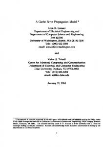
In an MMP, not only the metal cutting 共i.e., the machining operation兲, but also the setup operation 共part locating and orientation兲 affects part quality. The induced part error will propagate through the process, especially when operations correlate with each other. The main correlation is caused by the datum effect, i.e., if previous machined surfaces are used as the datum in the current operation, the datum imperfection often affects the accuracy of currently machined surfaces. Figure 1 shows the error propagation in a machining process with N operations. Operation k(k⫽1,...,N) is defined as the kth setup and the cutting operation based on that setup. In general, the number of machine stations can be smaller than the number of operations, because there may have been more than one setup operation within the same station. The main error sources at operation k are classified as: 1兲 fixture error ekf 共geometric inaccuracy of locating elements兲, 2兲 datum errors edk due to the imperfection of datum surfaces, 3兲 machine tool errors em k 共volumetric errors 关12兴兲, and 4兲 noise w(k) due to process natural variations. Assume that ekf , edk , em k and w(k) are independent. Setup error esk is the error jointly caused by ekf and edk in the kth setup operation. Machine tool error em k , often referred to as the tool path error, is the error generated by the kth cutting operation.

3

Part Model, Part Deviation, and Observation

Intermediate and final part deviation is of direct interest in modeling part dimensional error and error propagation. Part models

Journal of Manufacturing Science and Engineering Copyright © 2003 by ASME

MAY 2003, Vol. 125 Õ 255

Fig. 1 Error propagation in MMPs

need only to describe features relevant to part deviation. Therefore, a revised vectorial surface model is applied to represent the part. More details about vectorial surface modeling can be found in 关13兴. Part Model. Suppose a part has n surfaces related to the error propagation. Those n surfaces include surfaces to be machined, design datums, machining datums and measurement datums. In a coordinate system, the ith surface Xi can be described by its surface orientation ni ⫽ 关 n ix ,n iy ,n iz 兴 T , location pi ⫽ 关 p ix ,p iy ,p iz 兴 T , and size Di ⫽ 关 d i1 ,d i2 ,...,d im 兴 T . By stacking up ni , pi , and Di , Xi is represented as a vector with dimension (6⫹m), that is, Xi ⫽ 关 niT ,piT ,DiT 兴 共T6⫹m 兲 ⫻1

(1)

where m is the number of size parameters in Di . Size parameter here has broader meaning than that for the dimension of size given by GD&T 关14兴. It can be the diameter, flatness, or parallelism. With the representation for individual part surface, the part is modeled as a vector by stacking up all surface vectors, that is, X⫽ 关 XT1 ,XT2 ,...,XTn 兴 T

(2)

Part Deviation. Due to operational errors and natural process variation, machined part features might deviate from their ideal counterparts. The feature deviation can be derived from Eq. 共1兲, that is, the deviation of surface Xi from the ideal surface Xio 共in this paper, variable with superscript ‘‘o ’’ denotes the nominal value of that variable兲 is ⌬Xi ⫽ 关 ⌬niT ,⌬piT ,⌬DiT 兴 T

(3)

where ⌬ni ⫽ 关 ⌬n ix ,⌬n iy ,⌬n iz 兴 , ⌬pi ⫽ 关 ⌬p ix ,⌬p iy ,⌬p iz 兴 and ⌬Di ⫽ 关 ⌬d i1 ,⌬d i2 ,...,⌬d im 兴 T . An example for a cylinder surface is illustrated in Fig. 2. Let x denote part deviation ⌬X. By Eqs. 共2兲 and 共3兲, x is T

x⫽ 关 ⌬XT1 ,⌬XT2 ,...,⌬XTn 兴 T

T

(4)

Use x(k) to index the intermediate part deviation after operation k. Observation of Part Deviation. Suppose p part characteristics Y⫽ 关 Y 1 ,...,Y p 兴 T are measured. The deviation of Y from design specifications, i.e., ⌬Y⫽ 关 ⌬Y 1 ,...,⌬Y p 兴 T , represents the ob-

servations of part deviation x. Similarly, denote ⌬Y as y and index intermediate observation as y(k), if the measurement is taken at operation k. Y i (1⭐i⭐p) is a function of X, i.e., Y i ⫽G i (X). For example, Y i might be the distance between two planes. If part deviation x is small, Taylor series expansion can be used to approximate the function G i by a linear component Ci x plus a noise term ␯ i , that is, ⌬Yi ⫽Ci x⫹ ␯ i

(5)

where Ci ⫽ 关 dG i /dXT 兴 1⫻n ( 6⫹m ) and ␯ i includes the high order terms from Taylor series expansion and measurement errors. By Eq. 共5兲, y is expressed as y⫽Cx⫹ ␯

冋册

C1 C⫽ ] Cp

(6) (7)

p⫻n 共 6⫹m 兲

where C is defined as the sensitivity matrix, transforming the part deviation x to observed deviation y. ␯⫽ 关 ␯ 1 , ␯ 2 ,..., ␯ p 兴 T is the noise term.

4

Setup and Machining Operation

Part deviation is mainly caused by setup and machining operations. During each operation, the part is fixed in a fixture and then cut in the machine tool. Three coordinate systems are introduced as references to describe the part deviation and operational errors. Naturally the homogeneous transformation approach is applied to depict part transformation among coordinates and to model how the operational errors affect the part quality during the transformation. This is the main focus of this section, that is, kinematic modeling of machining and setup operations. 4.1

Coordinate Systems.

• M-Coordinate: the machine tool coordinate (x M ,y M ,z M ), in which the fixture is located and oriented on the machine table. • F-Coordinate: the fixture coordinate (x F ,y F ,z F ), built in the fixture in which the part is located and oriented. • P-Coordinate: the part coordinate (x,y,z), in which the part surfaces are represented. The subscription ‘‘P’’ is omitted for simplicity 共Fig. 3兲. Let X, XF and XM be the part represented in the P-Coordinate, F-Coordinate and M-Coordinate respectively. The homogeneous transformation is used to model the part transformation among coordinates through rotation and translation transformations. For example, before machining, the part needs to be fixed into a fixture on the machine tool table 共This operation is called setup and will be further discussed in Section 4.2兲. The procedure is modeled as transforming the part from P-Coordinate to F-Coordinate and then from F-Coordinate to M-Coordinate. The mathematical expression is given by Eq. 共8兲,

冋 册冋 XF ⫽ 1

Fig. 2 Cylinder surface and surface deviation representation

256 Õ Vol. 125, MAY 2003

F

RP 0

F

册冋 册

TP X 1 1

and

冋 册冋 XM ⫽ 1

M

RF 0

M

册冋 册

TF XF 1 1

(8)

Transactions of the ASME

Fig. 3 Coordinate systems

where ‘‘1’’ is a vector with all ones and ‘‘0’’ is zero matrix. Translation vector M TF is defined as

(9a) where (x F ,y F ,z F ) is the coordinate of the origin of the F-Coordinate in the M-Coordinate. Similarly, we have

(9b) where 共x,y,z兲 is the coordinate of the origin of the P-Coordinate in the F-Coordinate. Rotation matrix M R F is defined as

(10) where Rot F ⫽ 关 uF , vF , wF 兴 3⫻3 and uF , vF and wF denote three unit vectors pointing along the axes of the F-Coordinate in the M-Coordinate. I m⫻m is the identity matrix. F R P is defined as M

M

M

M

M

M

M

Fig. 4 Fixture with 3-2-1 locating scheme

The fact is that in the two-step procedure of setup, the fixture affects the coordinate transformation between the F-Coordinate and M-Coordinate, while the datum affects the coordinate transformation between the P-Coordinate and F-Coordinate. The part deviation might be generated due to improperly positioning the part in the M-Coordinate. To assess the impact of fixture errors and datum errors on part quality, we need to model fixture and datum and to study how those two types of errors affect setup. In order to illustrate fixture deviations, the study uses the popular 3-2-1 locating scheme 共Fig. 4兲. The same methodology can be followed for other locating schemes. Six fixture tooling elements Ti ’s (i⫽1,2, . . . ,6) are sufficient to restrict the six degrees of freedom of the part. In the contact area of tooling element Ti with the datum surface, the position of an arbitrary point is used to represent the position of Ti in the M-Coordinate, denoted as (T ix M ,T iy M ,T iz M ). Since T 1z M , T 2z M , T 3z M , T 4x M , T 5x M and T 6y M are sufficient to determine the F-Coordinate, a vector TE is defined to represent the fixture: TE ⫽ 关 T 1z M ,T 2z M ,T 3z M ,T 4x M ,T 5x M ,T 6y M 兴 T

The fixture deviation is caused by the deviations of tooling elements, which is defined as ⌬TE ⫽ 关 ⌬T 1z M ,⌬T 2z M ,⌬T 3z M ,⌬T 4x M ,⌬T 5x M ,⌬T 6y M 兴 T (14)

(11) where F Rot P ⫽ 关 F uP , F vP , F wP 兴 3⫻3 and F uP , F vP and F wP denote three unit vectors pointing along the axes of the P-Coordinate in the F-Coordinate. 4.2 Setup Operation. Setup consists of two steps, that is, position the workpiece on a fixture, and then locate the fixture on a machine tool table. Equation 共8兲 models the two-step procedure. An alternative is to model setup as a direct transformation from the P-Coordinate to the M-Coordinate. For the kth setup, the incoming workpiece X(k⫺1) is transformed to XM (k⫺1) in the M-Coordinate through a rotation transformation M R P (k) and a translation transformation M TP (k), that is, XM 共 k⫺1 兲 ⫽ M R P 共 k 兲 X共 k⫺1 兲 ⫹ M TP 共 k 兲 where M

M

R P (k) and

M

TP (k) can be obtained from Eq. 共8兲 as

R P 共 k 兲 ⫽ R F 共 k 兲 F R P 共 k 兲 and M

(12a)

M

TP 共 k 兲 ⫽ M R F 共 k 兲 F TP 共 k 兲 ⫹ M TF 共 k 兲

At operation k, only fixture TE 共indexed by TE (k)) affects M R F and M TF . Therefore, transformation deviation of M R F (k) and M TF (k) is caused by fixture deviation ⌬TE (k). Under a small deviation assumption, the transformation deviation is approximated by the first order Taylor series expansion, that is, ⌬ M R F共 k 兲 ⫽

R M 共 k 兲 ⫽ 共 M R P 共 k 兲兲 ⫺1 ⫽ 共 M R F 共 k 兲 F R P 共 k 兲兲 ⫺1 ⫽ P R F 共 k 兲 F R M 共 k 兲 (12c)

Journal of Manufacturing Science and Engineering

d 共 M R F 共 k 兲兲 i j ⌬TE 共 k 兲 dTE 共 k 兲 T

冋

册

(15a) n 共 6⫹m 兲 ⫻n 共 6⫹m 兲

d 共 M T F 共 k 兲兲 i ⌬TE 共 k 兲 dTE 共 k 兲 T

册

(15b) n 共 6⫹m 兲 ⫻1

where ( M R F (k)) i j denotes the ith row and the jth column of M R F (k), and ( M TF (k)) i denotes the ith row of M TF (k). As a result, the actual transformation from F-Coordinate to M-Coordinate is represented by the summation of a nominal transformation and the deviation caused by fixture errors, that is,

F

P

冋

⌬ M T F共 k 兲 ⫽

(12b) where F R P (k), F TP (k), M R F (k) and M TF (k) represent F R P , TP , M R F and M TF at operation k. The following relationship still holds:

(13)

F

M

R F 共 k 兲 ⫽ M R Fo 共 k 兲 ⫹⌬ M R F 共 k 兲

(16a)

M

TF 共 k 兲 ⫽ M TFo 共 k 兲 ⫹⌬ M TF 共 k 兲

(16b)

F

R P and TP are affected by datum. Before introducing datum deviation, we introduce a datum selection matrix D(k) as D 共 k 兲 ⫽diag共共 J 1 兲 共 6⫹m 兲 ⫻ 共 6⫹m 兲 , ¯ , 共 J n 兲 共 6⫹m 兲 ⫻ 共 6⫹m 兲 兲

(17)

MAY 2003, Vol. 125 Õ 257

where J i is a diagonal matrix only with ‘‘1’’ and/or ‘‘0’’ as data entries and m is the dimension of size parameters in X(k). From the incoming workpiece X(k⫺1), D(k) selects part surfaces used for datum at operation k. To select surface Xi as the primary datum, J i is constructed as diag(1,1,1,0 . . . 0), which specifies the orientation of the primary datum. For the secondary or the tertiary datum, J i is constructed by choosing the position component of a surface. Denote the datum as DE (k) with DE 共 k 兲 ⫽D 共 k 兲 X共 k⫺1 兲

⌬DE 共 k 兲 ⫽D 共 k 兲 x共 k⫺1 兲

(19)

If the datum DE (k) firmly contacts with tooling elements of fixture TE (k), the transformation matrices F R P (k) and F TP (k) are determined, which are functions of DE (k). Follow Eq. 共15兲, the deviation of F R P (k) and F TP (k) caused by ⌬DE (k) can be expressed as

冋

d 共 F R P 共 k 兲兲 i j ⌬DE 共 k 兲 dDE 共 k 兲 T

冋

册

(20a) n 共 6⫹m 兲 ⫻n 共 6⫹m 兲

d 共 F TP 共 k 兲兲 i ⌬DE 共 k 兲 ⌬ TP 共 k 兲 ⫽ dDE 共 k 兲 T F

册

(20b) n 共 6⫹m 兲 ⫻1

F

R P 共 k 兲 ⫽ F R oP 共 k 兲 ⫹⌬ F R p 共 k 兲

(21a)

F

TP 共 k 兲 ⫽ F ToP 共 k 兲 ⫹⌬ F TP 共 k 兲

(21b)

The joint effect of fixture errors and datum errors on setup can now be described by plugging Eqs. 共16兲 and 共21兲 into Eq. 共12兲. Neglecting high order terms, we have R P 共 k 兲 ⫽ M R Fo 共 k 兲 F R oP 共 k 兲 ⫹ 关 M R Fo 共 k 兲 ⌬ F R P 共 k 兲 ⫹⌬ M R F 共 k 兲 F R oP 共 k 兲兴 M

TP 共 k 兲 ⫽ 关

M

⫹ M R Fo 共 k 兲 ⌬ F TP 共 k 兲 ⫹⌬ M TF 共 k 兲兴 ⌬ R P共 k 兲 ⫽ M

M

M

(22b)

R Fo 共 k 兲 ⌬ F R P 共 k 兲 ⫹⌬ M R F 共 k 兲 F R oP 共 k 兲

⌬ TP 共 k 兲 ⫽⌬ R F 共 k 兲 M

F

B 共 k 兲 ⫽diag共共 I 1 兲 共 6⫹m 兲 ⫻ 共 6⫹m 兲 , ¯ , 共 I n 兲 共 6⫹m 兲 ⫻ 共 6⫹m 兲 兲 (24a) and (I i ) ( 6⫹m )( 6⫹m ) (1⭐i⭐n) is an indicator matrix for Xi , defined as I i⫽

再

I 共 6⫹m 兲 ⫻ 共 6⫹m 兲 ,

surface Xi is machined at operation k

0,

Otherwise (24b)

where I ( 6⫹m ) ⫻ ( 6⫹m ) is the identity matrix and ‘‘0’’ is the zero matrix. B(k) is a representation of the process sequence, while A(k) is defined as A(k)⫽I⫺B(k), labeling uncut surfaces at operation k. By transforming XM (k) back to the P-Coordinate, the part deviation is expressed as

u P共 em k 兲 i ⫽ 共 B 共 k 兲 xM 共 k 兲兲 i

(22d) Up to now, fixture error ekf and datum error edk can be explicitly expressed by Eqs. 共14兲 and 共19兲, i.e., ekf ⫽⌬TE (k) and edk ⫽⌬DE (k). Setup error e sk is expressed by Eqs. 共22c兲 and 共22d兲. 4.3 Machining Operation. After the setup operation transforms the workpiece X(k⫺1) to XM (k⫺1), the kth machining

(26)

Corresponding to the size parameters of surfaces, the size component of e m k represents tool size related errors. With this, the total part deviations induced by e m k are expressed as

(22c)

ToP 共 k 兲 ⫹ M R Fo 共 k 兲 ⌬ F TP 共 k 兲 ⫹⌬ M TF 共 k 兲

(25)

where noise term w(k) includes neglected high order error terms and natural process variation. In the M-Coordinate, only machine tool error e m k causes deviations of newly machined part surfaces B(k)XuM (k). Depending on the problem domains, e m k can be as complicated as the volumetric error model 关12兴, or a simplified kinematic machine tool model 关15兴. Since the purpose of this research is to model process variation propagation, distinguishing each machine tool error component is unnecessary. In this study, each surface deviation in B(k)xuM is treated as a projection of machine tool error e m k on that surface. The projections vary with surface orientations. Thus the projected machine tool error P(e m k ) i onto the ith surface (B(k)XuM (k)) i is represented as

(22a)

R Fo 共 k 兲 F ToP 共 k 兲 ⫹ M TFo 共 k 兲兴 ⫹ 关 ⌬ M R F 共 k 兲 F ToP 共 k 兲

(23)

where B(k) labels all surfaces to be machined at operation k, defined as

x共 k 兲 ⫽A 共 k 兲 x共 k⫺1 兲 ⫹B 共 k 兲 xu 共 k 兲 ⫹w共 k 兲

Similarly, the actual transformation from P-Coordinate to F-Coordinate is represented by the summation of a nominal transformation and the deviation caused by datum errors, that is,

M

XM 共 k 兲 ⫽A 共 k 兲 XM 共 k⫺1 兲 ⫹B 共 k 兲 XuM 共 k 兲

(18)

The datum deviation is represented as the deviation of those selected part surfaces, that is,

⌬ FR P共 k 兲 ⫽

operation generates new part XM (k), which can be divided into the machined surfaces B(k)XuM (k) and the uncut surfaces A(k)XM (k⫺1), that is,

B 共 k 兲 xuM 共 k 兲 ⫽B 共 k 兲关 X uM 共 k 兲 ⫺X oM 共 k 兲兴

(27)

Based on the knowledge of machine tool capability, we assume the deviation B(k)xuM (k) follows multivariate normal distribution.

5

Deviation Propagation Model

With the preparation work in Section 4, we are ready to describe how the datum errors, fixture errors, and machine tool errors cause part deviation for each operation 共Fig. 5兲. The result is

Fig. 5 Error propagation

258 Õ Vol. 125, MAY 2003

Transactions of the ASME

Fig. 6 Design specifications of cylinder head Table 1 Description of Characteristics Characteristics 共1兲 共2兲 共3兲 共4兲 共5兲 共6兲

Distance btw cover face M and datum surface D Distance btw joint face A and datum surface D Parallelism btw M and A Diameter of hole B Distance btw slot S and D Parallelism btw A and S

Specifications共mm兲

Operation

117.0⫾0.1 2.50⫾0.1 0.050 15.00⫾0.05 100.7⫾0.1 0.050

1st 2nd 3rd

given by the following proposition 共See the derivation in the Appendix兲. Proposition 1 The error propagation model in a MMP is proposed as

⫽C(k)x(k)⫹v(k). Hence, a state space model is developed to model the dimensional deviation propagation and observation for the machining process.

x共 k 兲 ⫽A 共 k 兲 x共 k⫺1 兲 ⫹ P R M 共 k 兲 B 共 k 兲 xuM 共 k 兲 ⫹ 关 P R M 共 k 兲 B 共 k 兲 M R oP 共 k 兲

6

⫺B 共 k 兲兴 X o 共 k 兲 ⫺ P R M 共 k 兲 B 共 k 兲 ⌬ M TP 共 k 兲 ⫹w 共 k 兲

(28)

By comparing Eq. 共28兲 with Eq. 共25兲, the machined surface deviation B(k)xu (k) at operation k can be represented as B 共 k 兲 xu 共 k 兲 ⫽ P R M 共 k 兲 B 共 k 兲 xuM 共 k 兲 ⫹ 关 P R M 共 k 兲 B 共 k 兲 M R oP 共 k 兲 ⫺B 共 k 兲兴 Xo 共 k 兲 ⫺ P R M 共 k 兲 B 共 k 兲 ⌬ M TP 共 k 兲

(29a)

Considering the impacts of datums and fixtures on setup 共Eqs. 共16兲 and 共21兲兲, we can rewrite Eq. 共29a兲 as B 共 k 兲 xu 共 k 兲 ⫽ P R Fo 共 k 兲 F R oM 共 k 兲 B 共 k 兲 xuM 共 k 兲 ⫹ 关 P R Fo 共 k 兲 ⌬ F R M 共 k 兲 B 共 k 兲 M R Fo 共 k 兲 F R oP 共 k 兲 Xo 共 k 兲 ⫺ P R Fo 共 k 兲 F R oM 共 k 兲 B 共 k 兲 ⌬ F R M 共 k 兲 F ToP 共 k 兲 ⫺ P R Fo 共 k 兲 F R oM 共 k 兲 B 共 k 兲 ⌬ M TF 共 k 兲兴 ⫹ 关 ⌬ P R F 共 k 兲 B 共 k 兲 F R oP 共 k 兲 Xo 共 k 兲 ⫺ P R Fo 共 k 兲 B 共 k 兲 ⌬ F TP 共 k 兲兴

(29b)

Remark 1 At the right hand side of Eq. 共29b兲, the three terms f d from left to right are caused by em k , ek and ek respectively. Since m f d ek , ek and ek are independent, those three terms are also independent. This suggests that B(k)xu (k) can be separated into three components corresponding to three types of errors. Remark 2 Although B(k)XuM (k) is only affected by the tool f d path movement, B(k)xu (k) can be contributed by em k , ek and ek . Remark 3 Equations 共28兲 and 共29兲 describe how the error sources affect part accuracy and how the errors propagate in the process. If we treat part deviation as a state vector, Eq. 共25兲, together with Eqs. 共28兲 and 共29兲, can be thought as a state equation. From Eq. 共6兲, deviation observation for operation k is written as y(k) Journal of Manufacturing Science and Engineering

Model Validation

A cylinder head is used to validate the proposed modeling methodology. The parts are machined under both normal and faulty conditions. The CMM measurements are compared with model predictions. Figure 6 shows the part design and specifications. Descriptions of the characteristics are given in Table 1. The association between characteristics and operations is illustrated by the first and the third column in Table 1. Three operations are performed to meet design specifications 共Table 2兲. Figure 7共a兲 graphically shows the operational sequence, where Ti ’s (i⫽1,2, . . . ,6) are six locators used as datums. The primary datum surface D consists of T1 , T2 and T3 . Surface M1 represents the cover face M after the first operation on it. The convention applies to other surfaces. Setups, fixtures and locating schemes are shown in Fig. 7共b兲. To obtain the repeatability of machine tools and fixtures, an experiment is conducted and the results are as follows: the standard deviation of the angular error component is 0.0001 radians and the standard deviation of the positional error component is 10 microns. The repeatability of size related errors is 20 microns. The fixture repeatability, i.e., the standard deviation of tooling element errors, is 10 microns. Under normal conditions, the real part was machined and the CMM measurement data is given in Table 5. Then a fault is pur-

Table 2 Operational Sequence and Locating Datums Locating Datums Operation # (Primary⫹Secondary⫹Tertiary datum) 1 2

D(T1 ,T2 ,T3 )⫹(T4 ,T5 )⫹T6 M1⫹(T4 ,T5 )⫹T6

3

A1⫹B⫹C

Operation Descriptions Mill cover M Mill joint face A Drill hole B and C Mill slot S

MAY 2003, Vol. 125 Õ 259

Fig. 7

„a… Operational sequence „b… fixture locating schemes & setups Table 3 Part Model

Xi 共1兲 共2兲 共3兲 共4兲 共5兲 共6兲

nx 共radian兲

ny 共radian兲

nz 共radian兲

px 共mm兲

py 共mm兲

pz 共mm兲

d1 共mm兲

0 0 0 0 0 0

0 0 0 0 0 0

1 1 1 1 1 1

⫺133.7 0 0 0 0 0

134.7 0 0 0 306 0

0 ⫺2.5 117.0 53.6 53.6 100.7

0 0 0 15 15 0

Surface D Joint face A Cover face M Hole B Hole C Slot S

Table 4 Setup Operations

Entry/unit

␣ ␤ ␥ px py pz

F-Coordinate to M-Coordinate 共nominal兲

P-Coordinate to F-Coordinate 共nominal兲

Fixture noise

Datum noise

Fixture fault

0 0 0 100 60 80

0 ␲ 0 0 0 0

0.0001 0.0001 0.0001 0.01 0.01 0.01

0.0001 0.0001 0.0001 0.01 0.01 0.01

⫺0.0020 ⫺0.0025 0.0001 0.01 0.01 0.4

radian mm

Table 5 Comparison between Measurement and Model Prediction „unit in mm… Char.#

共1兲

共2兲

共3兲

共4兲

共5兲

共6兲

Spec. CMM 共normal兲 Prediction 共normal兲 CMM 共fault兲 Prediction 共fault兲

117.0⫾0.1 117.096

2.50⫾0.1 2.457

0.05 0.035

15.0⫾0.05 15.034

100.7⫾0.1 100.726

0.05 0.042

117.048

2.495

0.028

15.000

100.603

0.035

117.053

2.320

0.446

15.038

100.816

0.446

117.052

2.349

0.144

15.002

100.931

0.202

posely introduced into operation 2 by putting a 0.3 mm shim onto a locating pin of the primary datum. Under faulty conditions, the second part was machined with CMM measurement given in Table 5. The model prediction is performed for comparison study. At first, the part model is built by following the rules given in Section 2. Six surfaces are chosen to model the part 共Table 3兲. The xoy plane of the P-Coordinate coincides with surface D. Different choices of P-Coordinate make no difference to the outcomes if the choice is consistent during the study. The data in Table 3 is the nominal values for the final operation which are determined by the process planning. The second step is to model the setup and machining operations. Under normal conditions, only natural variations exist. The fixture noise is generated by assuming that each tooling element follows a normal distribution with zero mean and standard deviation equal to its repeatability. From the process planning, Euler angles of ␣, ␤, and ␥ are used to construct rotation matrix M R F0 260 Õ Vol. 125, MAY 2003

and F R 0P (k), and p x , p y and p z are for M TFo and F ToP . Under faulty conditions, fixture errors are used to construct matrices ⌬ M R F and ⌬ M TF 共Described by Eq. 共15兲兲. ⌬ P R F and ⌬ F TP are caused by datum variations 共Described by Eq. 共20兲兲. In the first operation, the variability of datum targets Ti ’s (i⫽1,2,...,6) is given in Table 4. Random error of datum surface D is generated to take into account workpiece variations. Other datum surfaces used in the remaining operations are the direct output from the machining operations. The machining simulation is performed based on Eqs. 共28兲 and 共29兲. Developed with Matlab, the program runs in a Pentium III 533 computer with Windows 2000 operation system. 100 parts are run under both normal and faulty conditions. Each run takes less than 20 seconds. By comparing the predicted mean values of characteristics with CMM measurements 共Table 5兲, the discrepancies are small both under normal and faulty conditions. When the 0.3 mm shim is put onto one pin of the primary datum, the discrepTransactions of the ASME

ancies are relatively larger, e.g., the parallelism between M and A and the parallelism between A and S. As the shim makes the part tilted and increases the cutting depth, the cutting force and fixture stability problems could be the contributing factors that make parallelisms worse. Since those two factors are not modeled, this could be the main reason that explains the discrepancies. However, the model still is able to predict that parallelisms are beyond the tolerance range. As the deviations from tolerance are relatively smaller in real situations, the model predicts well within that area without extreme cutting conditions. Therefore, the discrepancies between model prediction and real measurements are reasonably small.

7

Summary

In this paper, a state space model was developed to model the error propagation in MMPs. This is achieved by • providing a quality-oriented part model: A revised vectorial surface model is applied to facilitate part deviation representation and observation. Only error transmission related surfaces are chosen to build the part model. • modeling setup, machining operations, and operational sequences: Modeling of setup, machining operations, and operational sequences facilitates deviation propagation analysis. Further, engineering knowledge from process planning can be captured. • considering errors from datums, fixtures, and machine tools: By using homogenous transformation approach, error transmission is captured by describing the kinematic relationships among three coordinate systems. Fixture errors are modeled in terms of tooling elements and a synthetic machine tool error model is proposed with consideration of both machine tool repeatability and the precision of cutting tool. • modeling deviation propagation: Part deviations are explicitly separated into three parts, i.e., deviations caused by upstream, fixtures, and machine tools. This separation is extremely important for the causality study and variation analysis.

3兲 Unload part from machine tool Part X(k) in P-Coordinate is X共 k 兲 ⫽ P R M 共 k 兲关 XM 共 k 兲 ⫺ M TP 共 k 兲兴 ⫽ P R M 共 k 兲 兵 A 共 k 兲关 M R P 共 k 兲 X共 k⫺1 兲 ⫹ M TP 共 k 兲兴 ⫹B 共 k 兲 XuM 共 k 兲 其 ⫺ P R M 共 k 兲 M Tp 共 k 兲 ⫽ P R M 共 k 兲 A 共 k 兲 M R P 共 k 兲 X共 k⫺1 兲 ⫹ P R M 共 k 兲 B 共 k 兲 XuM 共 k 兲 ⫹ P R M 共 k 兲共 k 兲 A 共 k 兲 M TP 共 k 兲 ⫺ P R M 共 k 兲关 A 共 k 兲 ⫹B 共 k 兲兴 M TP 共 k 兲 ⫽ P R M 共 k 兲 A 共 k 兲 M R P 共 k 兲 X共 k⫺1 兲 ⫹ P R M 共 k 兲 B 共 k 兲关 XuM 共 k 兲 ⫺ M TP 共 k 兲兴 As P R M (k) M R P (k)⫽I, we have P R M (k)A(k) M R P (k)⫽A(k). X(k) turns to be X共 k 兲 ⫽A 共 k 兲 X共 k⫺1 兲 ⫹ P R M 共 k 兲 B 共 k 兲关 XuM 共 k 兲 ⫺ M T P 共 k 兲兴 The part deviation after operation k is x(k)⫽X(k)⫺Xo (k). It is further expressed as x共 k 兲 ⫽A 共 k 兲 X共 k⫺1 兲 ⫹ P R M 共 k 兲 B 共 k 兲 b XuM 共 k 兲 ⫺ M T P 共 k 兲 c ⫺Xo 共 k 兲 ⫽A 共 k 兲 X共 k⫺1 兲 ⫹ P R M 共 k 兲 B 共 k 兲关 XuM 共 k 兲 ⫺XoM 共 k 兲 ⫹XoM 共 k 兲 ⫺ M TP 共 k 兲兴 ⫺ 关 A 共 k 兲 ⫹B 共 k 兲兴 Xo 共 k 兲 As operation k does not change A(k)X(k⫺1), A(k)Xo (k) ⫽A(k)Xo (k⫺1) holds. Then x共 k 兲 ⫽A 共 k 兲 x共 k⫺1 兲 ⫹ P R M 共 k 兲 B 共 k 兲关 XuM 共 k 兲 ⫺XoM 共 k 兲兴 ⫹ P R M 共 k 兲 B 共 k 兲 XoM 共 k 兲 ⫺ P R M 共 k 兲 B 共 k 兲 M TP 共 k 兲 ⫺B 共 k 兲 Xo 共 k 兲 As XoM (k)⫽ M R oP (k)Xo (k)⫹ M ToP (k) ⫺XoM (k), x(k) can be rewritten as

xuM (k)⫽XuM (k)

x共 k 兲 ⫽A 共 k 兲 x共 k⫺1 兲 ⫹ P R M 共 k 兲 B 共 k 兲 xuM 共 k 兲 ⫹ P R M 共 k 兲 B 共 k 兲关 M R oP 共 k 兲 Xo 共 k 兲 ⫹ M T oP 共 k 兲兴

Since the process variables are directly modeled, tolerance design can be performed without struggling on how to make assumptions about component dimensions. Besides that, design problems such as datum selection, fixture layout design, and process validation can also be studied based on the model. On the other hand, the model provides the basis to monitor the multioperational process and to determine root causes. Therefore, the proposed model has great potentials in a variety of applications.

⫺ P R M 共 k 兲 B 共 k 兲 M TP 共 k 兲 ⫺B 共 k 兲 Xo 共 k 兲 ⫽A 共 k 兲 x共 k⫺1 兲 ⫹ P R M 共 k 兲 B 共 k 兲 xuM 共 k 兲 ⫹ 关 P R M 共 k 兲 B 共 k 兲 M R oP 共 k 兲 ⫺B 共 k 兲兴 Xo 共 k 兲 ⫺ P R M 共 k 兲 B 共 k 兲关 M TP 共 k 兲 ⫺ M ToP 共 k 兲兴 ⫹w共 k 兲 Then we have Eq. 共28兲. w(k) is added process noise term.

Acknowledgment The authors gratefully acknowledge the financial support of the NSF Engineering Research Center for Reconfigurable Machining Systems 共NSF Grant EEC95-92125兲 at the University of Michigan and the valuable input from the Center’s industrial partners.

Appendix Proposition 1. The error propagation model in a MMP is proposed as x共 k 兲 ⫽A 共 k 兲 x共 k⫺1 兲 ⫹

and

P

R M 共 k 兲 B 共 k 兲 xuM 共 k 兲 ⫹ 关 P R M 共 k 兲 B 共 k 兲 M R oP 共 k 兲

Nomenclature ekf edk em k w(k)& ␯(k)

⫽ ⫽ ⫽ ⫽

X ⫽ X(k) ⫽

(28)

Y(k) ⫽ x(k) ⫽

Proof: For operation k, the following operations are performed in sequence: 1兲 Setup operation By Eq. 共12兲, setup operation is expressed as

xM , or xF ⫽

⫺B 共 k 兲兴 X o 共 k 兲 ⫺ P R M 共 k 兲 B 共 k 兲 ⌬ M TP 共 k 兲 ⫹w共 k 兲

XM 共 k⫺1 兲 ⫽ M R P 共 k 兲 X共 k⫺1 兲 ⫹ M TP 共 k 兲

y(k) ⫽ B(k) ⫽

2兲 Machining operation By Eq. 共23兲, XM (k) in M-Coordinate turns to be:

A(k) ⫽

XM 共 k 兲 ⫽A 共 k 兲 XM 共 k⫺1 兲 ⫹B 共 k 兲 XuM 共 k 兲

C(k) ⫽

Journal of Manufacturing Science and Engineering

fixture error at operation k datum error at operation k machine tool error at operation k noise terms in the state space equation for operation k a vector used to describe a part part machined after operation k, represented in the P 共part兲 coordinate part measurement at operation k deviation of X(k), represented in the P coordinate deviation of X, represented in the M 共Machine兲 coordinate or the F 共Fixture兲 coordinate deviation of Y(k) indicator matrix which labels all surfaces that are machined at operation k defined as A(k)⫽I⫺B(k), indicating surfaces not machined at operation k sensitivity matrix that relates x(k) to y(k) MAY 2003, Vol. 125 Õ 261

D(k) ⫽ datum selection matrix used to label the datum surfaces for operation k B(k)xu (k) ⫽ machined surface deviation at operation k Z o ⫽ nominal value of variable Z i R j (k) ⫽ rotation transformation from the j coordinate to the i coordinate at operation k,i, j⫽ P,F,M i T j (k) ⫽ translation transformation from the j coordinate to the i coordinate at operation ki, j⫽ P,F,M

References 关1兴 Fortini, E. T., 1967, Dimensioning for Interchangeable Manufacture, Industrial Press, NY. 关2兴 Gilson, J., 1951, A New Approach to Engineering Tolerances, The Machinery Publishing Co., London, UK. 关3兴 Greenwood, W. H., and Chase, K. W., 1987, ‘‘A New Tolerance Analysis Method for Designers and Manufactures,’’ ASME J. Ind., 109, pp. 112–116. 关4兴 Ding, Y., Jin, J., Ceglarek, D., and Shi, J., 2002, ‘‘Process-Oriented Tolerancing for Multi-Station Assembly System,’’ IIE Transactions on Design and Manufacturing 共to appear兲. 关5兴 Jin, J., and Shi, J., 1999, ‘‘State Space Modeling of Sheet Metal Assembly for Dimensional Control,’’ ASME J. Manuf. Sci. Eng., 121, pp. 756 –762. 关6兴 Ding, Y., Shi, J., and Ceglarek, D., 2002, ‘‘Diagnosability Analysis of Multi-

262 Õ Vol. 125, MAY 2003

关7兴 关8兴 关9兴 关10兴 关11兴 关12兴 关13兴 关14兴 关15兴

Station Manufacturing Processes,’’ ASME Transactions, Journal of Dynamics Systems, Measurement, and Control, Vol. 124, pp. 1–13. Mantripragada, R., and Whitney, D. E., 1999, ‘‘Modeling and Controlling Variation Propagation in Mechanical Assemblies Using State Transition Models,’’ IEEE Robotics and Automation , 15, pp. 124 –140. Lawless, J. F., Mackay, R. J., and Robinson, J. A., 1999, ‘‘Analysis of Variation Transmission in Manufacturing Processes—Part I,’’ J. Quality Technol., 31, pp. 131–142. Agrawal, R., Lawless, J. F., and Mackay, R. J., 1999, ‘‘Analysis of Variation Transmission in Manufacturing Processes—Part II,’’ J. Quality Technol., 31, pp. 143–154. Cai, W., Hu, S. J., and Yuan, J. X., 1997, ‘‘Variational Method of Robust Fixture Configuration Design for 3-D Workpiece,’’ ASME J. Manuf. Sci. Eng., 119, pp. 593– 602. Choudhuri, S. A., and De Meter, E. C., 1999, ‘‘Tolerance Analysis of Machining Fixture Locators,’’ ASME J. Manuf. Sci. Eng., 121, pp. 273–281. Chen, J. S., Yuan, J. X., Ni, J., and Wu, S. M., 1993, ‘‘Real-time Compensation for Time-variant Volumetric Errors on a Machining Center,’’ ASME J. Ind., 115, pp. 472– 479. Martinsen, K., 1993, ‘‘Vectorial Tolerancing for All Types of Surfaces,’’ ASME Advances in Design Automation, Vol. 2, pp. 187–198. ASME, Y14.5 M Dimensioning and Tolerancing, 1994. Frey, D. D., Otto, K. N., and Pflager, W., 1997, ‘‘Swept Envelopes of Cutting Tools in Integrated Machine and Workpiece Error Budgeting,’’ CIRP Ann., 46, pp. 475– 480.

Transactions of the ASME