PARTIAL MODEL CHECKING USING NETWORKS OF LABELLED ...

Logical Methods in Computer Science Vol. 9(4:1)2013, pp. 1–32 www.lmcs-online.org

Submitted Published

Sep. 28, 2012 Oct. 1, 2013

PARTIAL MODEL CHECKING USING NETWORKS OF LABELLED TRANSITION SYSTEMS AND BOOLEAN EQUATION SYSTEMS ´ ERIC ´ FRED LANG AND RADU MATEESCU Convecs team, Inria Grenoble – Rhˆ one-Alpes and Lig (Laboratoire d’Informatique de Grenoble), Montbonnot, France e-mail address: {Frederic.Lang,Radu.Mateescu}@inria.fr Abstract. Partial model checking was proposed by Andersen in 1995 to verify a temporal logic formula compositionally on a composition of processes. It consists in incrementally incorporating into the formula the behavioural information taken from one process — an operation called quotienting — to obtain a new formula that can be verified on a smaller composition from which the incorporated process has been removed. Simplifications of the formula must be applied at each step, so as to maintain the formula at a tractable size. In this paper, we revisit partial model checking. First, we extend quotienting to the network of labelled transition systems model, which subsumes most parallel composition operators, including m-among-n synchronisation and parallel composition using synchronisation interfaces, available in the E-Lotos standard. Second, we reformulate quotienting in terms of a simple synchronous product between a graph representation of the formula (called formula graph) and a process, thus enabling quotienting to be implemented efficiently and easily, by reusing existing tools dedicated to graph compositions. Third, we propose simplifications of the formula as a combination of bisimulations and reductions using Boolean equation systems applied directly to the formula graph, thus enabling formula simplifications also to be implemented efficiently. Finally, we describe an implementation in the Cadp (Construction and Analysis of Distributed Processes) toolbox and present some experimental results in which partial model checking uses hundreds of times less memory than on-the-fly model checking.

1. Introduction Concurrent safety critical systems can be verified using model checking [13], i.e., automatic evaluation of a temporal property against a formal model of the system. Although successful in many applications, model checking may face state explosion, particularly when the number of concurrent processes grows. State explosion can be tackled by divide-and-conquer approaches regrouped under the name compositional verification, which take advantage of the compositional structure of the concurrent system under verification. One such approach, which we call compositional model generation in this paper, consists in building the model of the system — usually an 2012 ACM CCS: [Software and its engineering]: Software creation and management—Software verification and validation—Formal software verification. Key words and phrases: automata, compositional verification, concurrency, model checking, temporal logic.

l

LOGICAL METHODS IN COMPUTER SCIENCE

DOI:10.2168/LMCS-9(4:1)2013

c F. Lang and R. Mateescu

CC

Creative Commons

2

F. LANG AND R. MATEESCU

Lts (Labelled Transition System) — in a stepwise manner, by successive compositions and minimisations modulo equivalence relations, possibly using interface constraints [26, 30] to avoid explosion of intermediate compositions. Tools using this approach [21, 31, 32, 15] are available in the Cadp (Construction and Analysis of Distributed Processes) [22, 23] toolbox. In this paper, we explore a dual approach named partial model checking, proposed by Andersen [2, 3] for concurrent processes running asynchronously and composed using Ccs parallel composition and restriction operators. For a modal µ-calculus [29] formula ϕ and a process composition P1 || . . . ||Pn , Andersen uses an operation ϕ//P1 called quotienting of the formula ϕ w.r.t. the process P1 , so that P1 || . . . ||Pn satisfies ϕ if and only if the smaller composition P2 || . . . ||Pn satisfies ϕ//P1 . In addition, simplifications can (and must) be applied to ϕ//P1 to reduce its size. Partial model checking is the incremental application of quotienting and simplifications, so that state explosion is avoided if the size of intermediate formulas can be kept sufficiently small. Partial model checking has been adapted and used successfully in various contexts, such as state-based models [5, 4], synchronous state/event systems [9], and timed systems [8, 11, 36, 37, 38]. It has also been specialised for security properties [40]. More recently, it has been generalised to the full Ccs process algebra, with an application to the verification of parameterised systems [7]. These various developments of partial model checking, although successful, were relatively scarce, which may be explained by the complexity of the method: obtaining a fully operational partial model checker requires a significant implementation effort and extensive experiments for fine-tuning and optimization. In this paper, we focus on partial model checking of the modal µ-calculus applied to (untimed) concurrent asynchronous processes. By considering only binary associative parallel composition operators (such as Ccs and Csp parallel compositions), previous works [2, 3, 7] are not directly applicable to more general operators, such as m-among-n synchronisation (where among n processes executing in parallel, any m of them must synchronise on a given action) and parallel composition by synchronisation interfaces (where all processes containing a given action in their synchronisation interface must synchronise on that action) [24], present in the E-Lotos standard and variants [12, 28]. Our first contribution in this paper is thus a generalisation of partial model checking to networks of Ltss [31], a general model that subsumes parallel composition, hiding, cutting, and renaming operators of standard process languages (Ccs, Csp, µCrl, Lotos, E-Lotos, etc.), including the above-mentioned parallel composition operators. Regarding the communication of data values, our approach is applicable to classical (i.e., with static communication) value-passing process algebras equipped with early operational semantics. This framework encompasses a significant fragment of the π-calculus (containing channel mobility and bounded process creation), which can be translated into classical value-passing process algebras [44]. In realistic cases, partial model checking handles huge formulas and processes, thus requiring efficient implementations. Our second contribution is a reformulation of quotienting as a synchronous product (which can itself be represented in the network model) between a graph representing the formula (called a formula graph) and the behaviour graph of a process, thus enabling efficient implementation using existing tools dedicated to graph manipulations. We prove that this reformulation is sound. Our third contribution is the reformulation of formula simplifications as a combination of graph reductions (including minimisations modulo equivalence relations and bisimulations) and partial evaluation of the formula graph using a Bes (Boolean Equation System) [1].

PARTIAL MODEL CHECKING USING NETWORKS OF LTS AND BOOLEAN EQUATION SYSTEMS

3

Verifying modal µ-calculus formulas of arbitrary alternation depth is generally exponential in the size of the process graph, while verifying the alternation-free fragment remains of linear complexity. Our fourth contribution is a specialisation of the technique to alternationfree µ-calculus formulas. We also present how this specialisation can be again generalised to handle also useful fairness operators of alternation 2 in linear time without developing the complex machinery to evaluate general alternation-2 µ-calculus formulas. Finally, we present an implementation in Cadp and a case-study that illustrates the complementarity between partial and on-the-fly model checking. Paper Overview. The modal µ-calculus is presented in Section 2. The network of Ltss model is presented in Section 3. The generalisation of quotienting to networks and its reformulation as a synchronous product is presented in Section 4. The simplification rules are presented in Section 5. The rules specific to alternation-free µ-calculus formulas are presented in Section 6. The way we handle fairness operators is presented in Section 7. Our implementation of partial model checking of the regular alternation-free µ-calculus extended with fairness operators is presented in Section 8. Experimental results are presented in Section 9. Concluding remarks are given in Section 10. This paper is an extended version of an earlier paper [34]. 2. The Modal µ-Calculus We consider systems whose behavioural semantics can be represented using an Lts (Labelled Transition System), and whose properties can be expressed in the modal µ-calculus [29]. Definition 2.1 (Lts). An Lts is a tuple (Σ, A, −→, s0 ), where: • Σ is a set of states, • A is a set of labels, • −→ ⊆ Σ × A × Σ is the (labelled) transition relation, • and s0 ∈ Σ is the initial state. a a For an Lts S = (Σ, A, −→, s0 ), we may also write s−→s′ ∈ S (or simply s−→s′ when S is clear from the context) instead of (s, a, s′ ) ∈ →. Definition 2.2 (Syntax of the modal µ-calculus). The modal µ-calculus formulas (ϕ) are terms built from Boolean constants (ff , tt), Boolean connectors (disjunction ∨, conjunction ∧, and negation ¬), modalities (possibility h i and necessity [ ]), and fix-point operators (minimal µ and maximal ν) over propositional variables X, generated by the following grammar: ϕ ::= ff | ϕ1 ∨ ϕ2 | hai ϕ0 | µX.ϕ0 | tt | ϕ1 ∧ ϕ2 | [a] ϕ0 | νX.ϕ0 | ¬ϕ0 | X To ensure a proper definition of fix-point operators, a commonly adopted and sufficient condition is that formulas ϕ are syntactically monotonic [29], i.e., have an even number of negations on every path between a variable occurrence X and the µ or ν operator that binds X. Therefore, we will only consider syntactically monotonic formulas. We write Lµ for the set of µ-calculus formulas. We write fv (ϕ) for the set of variables free in ϕ, and bv (ϕ) for the set of variables bound in ϕ. We call a closed formula any formula ϕ such that fv (ϕ) = ∅. We assume that

4


[[ff ]] ρ = ∅ [[tt]] ρ = Σ [[ϕ1 ∨ ϕ2 ]] ρ = [[ϕ1 ]] ρ ∪ [[ϕ2 ]] ρ [[ϕ1 ∧ ϕ2 ]] ρ = [[ϕ1 ]] ρ ∩ [[ϕ2 ]] ρ a [[hai ϕ0 ]] ρ = {s ∈ Σ | (∃s′ ∈ Σ) s−→s′ ∧ s′ ∈ [[ϕ0 ]] ρ} a [[[a] ϕ0 ]] ρ = T {s ∈ Σ | (∀s′ ∈ Σ) s−→s′ =⇒ s′ ∈ [[ϕ0 ]] ρ} [[µX.ϕ0 ]] ρ = S{U ⊆ Σ | [[ϕ0 ]] (ρ ⊘ [U/X]) ⊆ U } [[νX.ϕ0 ]] ρ = {U ⊆ Σ | U ⊆ [[ϕ0 ]] (ρ ⊘ [U/X])} [[¬ϕ0 ]] ρ = Σ \ [[ϕ0 ]] ρ [[X]] ρ = ρ(X) Figure 1: Semantics of the modal µ-calculus all bound variables have distinct names, and for X ∈ bv (ϕ), we write ϕ[X] for the (unique) sub-formula of ϕ of either form µX.ϕ0 or νX.ϕ0 . Given ϕ1 and ϕ2 , we write ϕ1 [ϕ2 /X] for substituting all free occurrences of X in ϕ1 by ϕ2 (while implicitly applying α-conversion to maintain the unicity of bound variables). Definition 2.3 (Semantics of the modal µ-calculus). The semantics of the modal µ-calculus are formally defined by the equations of Figure 1. A propositional context ρ is a partial function mapping propositional variables to sets of states and ρ ⊘ [U/X] stands for a propositional context identical to ρ except that X is mapped to U . The interpretation [[ϕ]] ρ (also written [[ϕ]] if ρ is empty) of a state formula on an Lts in a propositional context ρ (which maps each variable free in ϕ to a set of states) denotes the subset of states satisfying ϕ in that context. The Boolean connectors are interpreted as usual in terms of set operations. The possibility modality hai ϕ0 (resp. the necessity modality [a] ϕ0 ) denotes the states for which some (resp. all) of their outgoing transitions labelled by a lead to states satisfying ϕ0 . The minimal fix-point operator µX.ϕ0 (resp. the maximal fix-point operator νX.ϕ0 ) denotes the least (resp. greatest) solution of the equation X = ϕ0 interpreted over the complete lattice 2Σ , ∅, Σ, ∩, ∪, ⊆ . A state s satisfies a closed formula ϕ if and only if s ∈ [[ϕ]]. Proposition 2.4. The modal µ-calculus satisfies the following identities: ¬tt ¬ff ¬(ϕ1 ∧ ϕ2 ) ¬(ϕ1 ∨ ϕ2 ) ¬ [a] ϕ0 ¬ hai ϕ0 ¬νX.ϕ0 ¬µX.ϕ0

= = = = = = = =

ff tt ¬ϕ1 ∨ ¬ϕ2 ¬ϕ1 ∧ ¬ϕ2 hai ¬ϕ0 [a] ¬ϕ0 µX.¬ϕ0 [¬X/X] νX.¬ϕ0 [¬X/X]

Definition 2.5 (Positive form and disjunctive form). Every modal µ-calculus formula ϕ can be rewritten in both of the following forms: • A formula is in positive form if it contains any of the modal µ-calculus operators but the negation operator ¬. Note that syntactic monotonicity implies that every negation can be eliminated using the identities of Proposition 2.4. Given a modal µ-calculus formula ϕ, we write ϕ+ the corresponding formula in positive form.


5

• A formula is in disjunctive form if it contains only the constant ff , disjunctions, possibility modalities, minimal fix-points, propositional variables and negations. Every formula can be put in disjunctive form using the identities of Proposition 2.4. Note that a formula in disjunctive form is not necessarily a disjunctive formula due to the presence of negations. Definition 2.6. A formula ϕ is alternation-free if ϕ+ does not contain any sub-formula of the form µX.ϕ1 (resp. νX.ϕ1 ) containing a sub-formula of the form νY.ϕ2 (resp. µY.ϕ2 ) such that X ∈ fv (ϕ2 ). The fix-point sign of a variable X in ϕ is µ (resp. ν) if ϕ+ [X] has the form µX.ϕ0 (resp. νX.ϕ0 ). We write Lµ1 for the set of alternation-free µ-calculus formulas, and more generally Lµn for the set of µ-calculus formulas of alternation up to n (for some n). Definition 2.7 (Block-labelled formula). In this paper, we consider block-labelled formulas ϕ in disjunctive form, in which each propositional variable X is labelled by a natural number k, called its block number. Intuitively, a block-labelling is well-formed if the µ-calculus formula can be converted into an equivalent set of µ-calculus equations partitioned into blocks, so that all variables having the same block number are defined in the same block and if k < k′ then the equations within block number k occur before the equations within block number k′ . The proof is beyond the scope of this paper. The well-formedness conditions are the following: (1) All occurrences of a given variable X are labelled by the same block number k. (2) All variables sharing the same block number have the same fix-point sign. ′ (3) For all X k ∈ bv (ϕ), Y k ∈ fv(ϕ[X k ]) it holds that k′ ≤ k. By convention, we assume without loss of generality that the even block numbers are associated to variables of sign µ and odd block numbers are associated to variables of sign ν. Initially, every unlabelled formula ϕ in disjunctive form can be turned into the wellformed block-labelled formula bl (ϕ, tt, 0, []), where bl (ψ, b, k, γ) is defined as follows, γ denoting a mapping from variables to block numbers: bl (ff , b, k, γ) bl (X, b, k, γ) bl (¬ϕ0 , b, k, γ) bl (ϕ1 ∨ ϕ2 , b, k, γ) bl (hai ϕ0 , b, k, γ)

= = = = =

ff X γ (X) ¬bl (ϕ0 , ¬b, k, γ) bl (ϕ1 , b, k, γ) ∨ bl (ϕ2 , b, k, γ) hai bl (ϕ0 , b, k, γ) µX k .bl (ϕ0 , tt, k, γ[X 7→ k]) if b = tt bl (µX.ϕ0 , b, k, γ) = k+1 µX .bl (ϕ0 , tt, k + 1, γ[X 7→ k + 1]) otherwise

We write blocks(ϕ) for the set of block numbers occurring in ϕ. A block-labelled formula ϕ ′ in disjunctive form is alternation-free if k′ = k for all X k ∈ bv(ϕ), Y k ∈ fv(ϕ[X k ]). A well-known result of the µ-calculus is that the variables of an alternation-free formula can be partitioned into blocks that have no cyclic dependencies. Another way to state this result is that any unlabelled formula in disjunctive form is alternation-free if and only if it can be block-labelled so that it satisfies the definition of alternation-free block-labelled formula. In the remainder of this paper, we will consider block-labelled formulas in disjunctive form. At last, we consider the following notion of formula equivalence, which is a slight generalisation of syntactic equality to enclose also the semantic notions of renaming, commutativity, and idempotence.

6


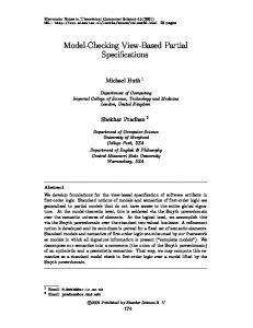
Definition 2.8. Let f be a bijective function from the set of propositional variables to itself, called a renaming. For formulas in disjunctive form, we define syntactic equality modulo commutativity, idempotence and f -renaming as the smallest relation, written =f , such that if ϕi =f ϕ′i (i ∈ 0..2) then: • ff =f ff , ¬ϕ0 =f ¬ϕ′0 , hai ϕ0 =f hai ϕ′0 , ϕ1 ∨ ϕ2 =f ϕ′1 ∨ ϕ′2 , X =f f (X), and µX.ϕ0 =f µf (X).ϕ′0 for each propositional variable X (syntactic equality modulo renaming), • ϕ1 ∨ ϕ2 =f ϕ′2 ∨ ϕ′1 (commutativity), • ϕ0 ∨ ϕ0 =f ϕ′0 and ϕ0 =f ϕ′0 ∨ ϕ′0 (idempotence). 3. Networks of LTSs Networks of LTSs (or networks for short) are inspired from the Mec [6] and Fc2 [10] synchronisation vectors and were introduced in [31] as an intermediate model to represent compositions of Ltss using various operators. Definition 3.1 (Vector and vector projection). We write n..m for the set of integers ranging from n to m, or the empty set if n > m. A vector v of size n is a total function on 1..n. For i ∈ 1..n, we write v[i] for v applied to i, denoting the element of v stored at index i. We write (e1 , . . . , en ) for the vector v of size n such that (∀i ∈ 1..n) v[i] = ei . In particular, () denotes a vector of size 0. Given n ≥ 1 and i ∈ 1..n, v\i denotes the projection of v on to the set of indices 1..n \ {i}, defined as the vector of size n − 1 such that (∀j ∈ 1..i − 1) v\i [j] = v[j] and (∀j ∈ i..n − 1) v\i [j] = v[j + 1]. Definition 3.2 (Network of LTSs). A network of LTSs N of size n is a pair (S, V ), where S is a vector of Ltss (called individual LTSs) of size n, and V is a set of synchronisation rules. Each synchronisation rule has the form (t, a) with a a label and t a vector of size n, called the synchronisation vector, of labels and occurrences of a special symbol • distinct from any label. Let S[i] = (Σi , Ai , −→i , s0i ) (i ∈ 1..n). N can be associated to a (global) Lts lts (N ) which is the parallel composition of individual Ltss. Each (t, a) ∈ V defines transitions labelled by a, obtained either by synchronisation (if more than one index i is such that t[i] 6= •) or by interleaving (otherwise) of individual Lts transitions. Formally, lts (N ) = (Σ, A, −→, s0 ), where: • Σ = Σ1 × . . . × Σn , • A = {a | (t, a) ∈ V }, • s0 = (s01 , . . . , s0n ), and a • −→ is the relation satisfying s−→s′ if and only if there exists (t, a) ∈ V such that for all i ∈ 1..n: ′ s [i] = s[i] if t[i] = • t[i] s[i]−→i s′ [i] otherwise We write A(t) for the set of active Lts (indices), defined by {i | i ∈ 1..n ∧ t[i] 6= •}. Example 3.3. Let a, b, c, and d be labels, and P1 , P2 , and P3 be the processes defined in Figure 2 (top), where the initial states are denoted by bold circles. Let N = ((P1 , P2 , P3 ), V ) with V = {((a, a, •), a), ((a, •, a), a), ((b, b, b), b), ((c, c, •), τ ), ((•, •, d), d)}, whose global Lts is depicted in Figure 2 (bottom left). The first two rules express a nondeterministic synchronisation on a between either P1 and P2 , or P1 and P3 . The third rule expresses a


0

c

c

3

a

b 1

a

1

τ

1

3

c

3

b

6

τ

d 2

d

4

9

5

0

11

c

a 1

3

d

b

2

a αa τ

1

4

τ αb

3

6

αb τ

7

10

τ

12

lts (N )

a

13

τ

τ

5

a

8

5

7

9

αa τ

11

αa

a b

4

P3

d τ

d τ

8

d

2

a

5

b

b

0

P2

a τ

4 a

P1 0

c

2

a

2

c

b

0

7

14

10

lts (N\3 )

Figure 2: Labelled Transition Systems for N defined in Example 3.3 multiway synchronisation on b. The fourth rule yields an internal (τ ) transition. The fifth rule expresses full interleaving of transitions labelled by d. The network of Ltss model is used in the tool Exp.Open [31] of Cadp as an intermediate model for representing Ltss composed using the hiding, renaming, cutting, and parallel composition operators present in the process algebras Ccs, Csp, Lotos, and µCrl, but also more expressive operators, such as m-among-n synchronisation and parallel composition using synchronisation interfaces [24] present in E-Lotos [28] and Lotos NT [12]. For instance, the rules {((a, a, •), a), ((a, •, a), a), ((•, a, a), a)} realize 2-among-3 synchronisation on a. Computing the interactions of a process Pi with its environment in a composition of processes ||j∈1..n Pj is easy when || is a binary and associative parallel composition operator, since ||j∈1..n Pj = Pi || (||j∈1..n\{i} Pj ). However, as argued in [24], binary and associative parallel composition operators are of limited use when considering, e.g., m-among-n synchronisation. A more involved operation named sub-network extraction is necessary for networks. Definition 3.4 (Sub-network extraction). N = (S, V ) being a network of size n, we assume a function α (t, a) that assigns a unique unused label to each (t, a) ∈ V . Given i ∈ 1..n, we define N\i = (S\i , V\i ) the sub-network of N modeling the environment of S[i] in N , where V\i = {(t\i , a) | (t, a) ∈ V ∧ i ∈ / A(t)} ∪ {(t\i , α (t, a)) | (t, a) ∈ V ∧ {i} ⊂ A(t)}. N is semantically equivalent to the network ((S[i], lts (N\i )), V ′ ) with V ′ the following set of rules, which define the interactions between S[i] and N\i : { ((•, a), a) | (t, a) ∈ V ∧ i ∈ / A(t) }∪ { ((t[i], α (t, a)), a) | (t, a) ∈ V ∧ {i} ⊂ A(t) } ∪ { ((a, •), a) | (t, a) ∈ V ∧ {i} = A(t) } Each α(t, a) is a unique interaction label between S[i] and N\i , which aims at avoiding erroneous interactions in case of nondeterministic synchronisation.

8


Example 3.5. N being defined in Example 3.3, N\3 has vector of Ltss (P1 , P2 ), P1 and P2 being defined in Figure 2 (top left and top middle), and rules {((a, a), a), ((a, •), αa ), ((b, b), αb ), ((c, c), τ )} with αa = α ((a, •, a), a) and αb = α ((b, b, b), b); lts(N\3 ) is depicted in Figure 2 (bottom right); Composing it with P3 using {((•, a), a), ((a, αa ), a), ((b, αb ), b), ((•, τ ), τ ), ((d, •), d)} yields lts(N ). Note that if a had been used instead of αa in the above synchronisation rules, then the composition of N\3 with P3 would have enabled, in addition to the (correct) binary synchronisations on a between P1 and P2 and between P1 and P3 , the (incorrect) multiway synchronisation on a between the three of P1 , P2 , and P3 . Indeed, the label a resulting from the synchronisation between P1 and P2 in N\3 — rule ((a, a), a) in N\3 — could synchronise with the label a in P3 — rule ((a, a), a) in the composition between N\3 and P3 . Note however that t[i] can be used instead of α(t, a) when the network does not have nondeterministic synchronisation on t[i], as is the case for b and αb in this example. In this paper we use α(t, a) uniformly to avoid complications. 4. Quotienting for Networks using Networks To check a closed formula ϕ on a network N = (S, V ), one can choose an individual Lts S[i], compute the quotient of the formula ϕ with respect to S[i], and check the resulting quotient formula on the smaller (at least in number of individual Ltss, but also hopefully in global Lts size) network N\i . Definition 4.1 (Quotient formula). The quotient formula is written ϕ //∅i si0 and defined as follows for closed formulas in disjunctive form: ff //B i s = ff k B X k //B i s = ϕ[X ] //i s B (¬ϕ0 ) //B i s = ¬(ϕ0 //i s) B B (ϕ1 ∨ ϕ2 ) //B i s = (ϕ1 //i s) ∨ (ϕ2 //i s) ( Xsk (µX k .ϕ0 ) //B B∪{Xsk } i s = µXsk .(ϕ0 //i s)  ( i∈ / A(t) W  (haiϕ ) //B s =  ({i} ⊂ A(t) 0

i

(t,a)∈V

if Xsk ∈ B otherwise

∧W hai (ϕ0 //B i s) ) ′ hα (t, a)i (ϕ0 //B ∧ t[i] i s )) Ws−→i s′ ′ (ϕ0 //B ({i} = A(t) ∧ t[i] i s )) ′ s−→i s

 ∨ ∨  

This definition follows and generalises Andersen’s [2] (specialised for Ccs) to networks. The main difference is the definition of (haiϕ0 ) //B i s, Ccs composition corresponding to vectors ((a, •), a), ((•, a), a), or ((a, a), τ ), a and a being an action and its Ccs co-action, making the use of special labels α(t, a) not necessary. A minor difference is that we use µ-calculus terms instead of equations1. Any sub-formula produced by quotienting has the 1Note that terms will be compiled into graphs, thus enabling the sharing of sub-formulas that is also

possible using equations.


9

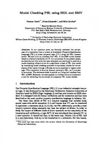
same block number as the original sub-formula, reflecting the order of equation blocks in Andersen’s definition. The set B keeps track of new variables already introduced in the quotient formula. Quotienting is well-defined, because formulas are finite, every ϕ[X k ] has the form µX k .ϕ0 (because the formula is in disjunctive form), and the size of the set B is bounded by | bv (ϕ)| × |Σi |. Note that well-formedness of the block-labelling is preserved by quotienting, because for every variable Xsk ∈ bv (ϕ //∅i s0 ) we have X k ∈ bv (ϕ) and for ′ ′ every variable Ysk′ ∈ fv ((ϕ //∅i s0 )[Xsk ]) we have Y k ∈ fv (ϕ[X k ]), and therefore k′ ≤ k. Example 4.2. The µ-calculus formula µX 0 .haitt∨hbiX 0 (existence of a path of zero or more b leading to an a) can be rewritten to disjunctive form as µX 0 .hai¬ff ∨ hbiX 0 . Quotienting of this formula with respect to P3 in the network N introduced in Example 3.3 (page 6) yields the formula µX00 .hai¬ff ∨ hαa i¬ff ∨ hαb iµX20 .hai¬ff ∨ ff . In other words, an action a can be reached after a (possibly empty) sequence of b actions in the network N if and only if an action a, or an action αa , or an action αb followed by an action a, can be reached immediately in N\3 , given the behaviour of P3 depicted in Figure 2 (page 7). We now show that quotienting can be implemented as a network that realises a product between an Lts encoding the formula (called a formula graph) and an individual Lts of the network under verification. Definition 4.3 (Circuit). Let S = (Σ, A, →, s0 ) be an Lts and T ⊆ → be a subset of its transitions. The states of T are defined as the set st (T ) = {s, s′ ∈ Σ | (s, σ, s′ ) ∈ T }. T is a circuit of S if for all s, s′ ∈ st (T ) there is a sequence of transitions belonging to T from s to s′ . A state s ∈ st (T ) is a root of the circuit T if there is a sequence of transitions from s0 to s that does not traverse any transition of T . Definition 4.4 (Formula graph). A formula graph is an Lts (Σ, A, →, s0 ) such that: (1) Every label σ ∈ A has either form ∨, ¬, hai (for some a belonging to a fixed set of action names), or µk (for some k ∈ N). µk ′ δ (2) If s0 −→s−→s for some δ ∈ A∗ and k ∈ N, then k is even if and only if δ contains an even number of occurrences of the label ¬. (3) If s ∈ Σ is a root of a circuit then (a) the circuit contains a µk -transition and (b) if the first µk -transition traversed on the circuit starting in s has block number k′ then every µk -transition belonging to the circuit satisfies k ≥ k′ . Every formula graph can be decoded into a closed formula as follows. Definition 4.5 (Decoding a formula graph). A formula graph P = (Σ, A, →, s0 ) encodes the modal µ-calculus formula decs (P, s0 , ∅), where decs (P, s, E) is defined as follows (E ⊆ Σ). In our decoding every variable is uniquely identified by the source state s and the block number k of the µ-transition, which we write sk . _ σ decs (P, s, E) = dect (P, s−→s′ , E) σ

s−→s′ ∈P

where

∨

dect (P, s−→s′ , E) = decs (P, s′ , E) ¬ dect (P, s−→s′ , E) = ¬ decs (P, s′ , E) hai dect (P, s−→s′ , E) = hai decs (P, s′ , E) k µk ′ s dect (P, s−→s , E) = µsk . decs (P, s′ , E ∪ {s})

if s ∈ E otherwise

10


4

hbi

∨

2

5

∨ 0

µ0

¬

µ0

0

6

1

3

2

hαb i

4

∨

∨

hai ∨

∨

1

9

¬

6

hai

3

7

µ0

10

∨

11

∨

hαa i

5

¬

(a)

8

12

hai

13

¬

14

(b) hαb i 0

hai 1

¬ 2

3

hai hαa i

(c) Figure 3: Examples of formula graphs This definition implies that a deadlock state decodes as ff (empty disjunction). Function decs is well-defined. In particular, it terminates because every cyclic path contains a label of the form µk . By recording in the set E the source states of traversed µk -transitions, we thus avoid infinite traversals of cycles. In practice (see next section), formula graphs need not be decoded except for correctness proofs. Definition 4.6 (Encoding a formula into a formula graph). The formula graph corresponding to a formula ϕ in disjunctive form is an Lts written enc (ϕ), whose states are identified with sub-formulas of ϕ. The initial state of the formula graph is ϕ, ff is a deadlock state, and each sub-formula has transitions as follows: hai ∨ ¬ ¬ϕ0 −→ϕ0 haiϕ0 −→ϕ X k −→ϕ[X k ] 0 µk ∨ ∨ ϕ1 ∨ ϕ2 −→ϕ1 ϕ1 ∨ ϕ2 −→ϕ2 µX k .ϕ0 −→ϕ0 Although the states of a formula graph are identified by formulas, only the transition labels are required for decoding. In figures, states will be simply identified by numbers. Note that the formula graph obtained by encoding a formula satisfies the conditions given in Definition 4.4. Condition (2) is a direct consequence of the block-labelling convention stated in Definition 2.7. Condition (3) comes from the fact that the roots of the circuits are the states associated to formulas of the form µX k .ψ such that X k occurs free in ψ. In particular, subcondition (b) is a consequence on the third well-formedness condition given in Definition 2.7. Example 4.7. The formula graph corresponding to the formula µX 0 .(haitt) ∨ hbiX 0 introduced in Example 4.2 is depicted in Figure 3 (a). We now prove that our encoding of closed formulas into formula graphs is sound, in the sense that the formula can be recovered from the formula graph into which the formula is encoded. This is stated formally in Proposition 4.9 below, which is a corollary of the following Lemma: Lemma 4.8. Let ϕ be a closed formula in disjunctive form and f be a renaming that maps k

each propositional variable X k ∈ bv (ϕ) to ϕ[X k ] . For every sub-formula ψ of ϕ, if {ϕ[Y k ] | Y k ∈ fv (ψ)} ⊆ E and E ∩ {ϕ[Y k ] | Y k ∈ bv (ψ)} = ∅, then decs (enc (ϕ), ψ, E) =f ψ. Proof. We proceed by structural induction on ψ:

PARTIAL MODEL CHECKING USING NETWORKS OF LTS AND BOOLEAN EQUATION SYSTEMS 11

Case ψ = ff: By definition of enc (ϕ), the state ψ has no outgoing transition. Therefore by definition of decs , we have decs (enc (ϕ), ff , E) = ff . ∨

Case ψ = X k : By definition of enc (ϕ), the state ψ has a single transition X k −→ϕ[X k ]. Therefore by definition of decs , we have decs (enc (ϕ), X k , E) = decs (enc (ϕ), ϕ[X k ], E). Since X k ∈ fv (X k ), by the hypothesis ϕ[X k ] ∈ E. It follows by definition of decs that k

decs (enc (ϕ), X k , E) = ϕ[X k ] =f X k . ¬

Case ψ = ¬ψ0 : By definition of enc (ϕ), the state ψ has a single transition ¬ψ0 −→ψ0 . Therefore by definition of decs , we have decs (enc (ϕ), ¬ψ0 , E) = ¬ decs (enc (ϕ), ψ0 , E). Since fv (ψ0 ) = fv (ψ) and bv(ψ0 ) = bv (ψ), the induction hypothesis holds and then decs (enc (ϕ), ψ0 , E) =f ψ0 . It follows immediately that decs (enc (ϕ), ¬ψ0 , E) =f ¬ψ0 . ∨

Case ψ = ψ1 ∨ ψ2 : By definition of enc (ϕ), the state ψ has two transitions ψ1 ∨ ψ2 −→ψ1 ∨ and ψ1 ∨ ψ2 −→ψ2 . Therefore by definition of decs , we have decs (enc (ϕ), ψ1 ∨ ψ2 , E) = decs (enc (ϕ), ψ1 , E) ∨ decs (enc (ϕ), ψ2 , E) (modulo commutativity if the transitions are enumerated in the opposite order, and idempotence if the transitions are identical). Since fv (ψ1 ) ∪ fv (ψ2 ) = fv (ψ) and bv(ψ1 ) ∪ bv (ψ2 ) = bv (ψ), the induction hypothesis holds and then we have both decs (enc (ϕ), ψ1 , E) =f ψ1 and decs (enc (ϕ), ψ2 , E) =f ψ2 . It follows that decs (enc (ϕ), ψ1 ∨ ψ2 , E) =f ψ1 ∨ ψ2 . hai

Case ψ = haiψ0 : By definition of enc (ϕ), the state ψ has a single transition haiψ0 −→ψ0 . Therefore by definition of decs , we have decs (enc (ϕ), haiψ0 , E) = hai decs (enc (ϕ), ψ0 , E). Since fv (ψ0 ) = fv (ψ) and bv(ψ0 ) = bv (ψ), the induction hypothesis holds and then decs (enc (ϕ), ψ0 , E) =f ψ0 . It follows immediately that decs (enc (ϕ), haiψ0 , E) =f haiψ0 . µk

Case ψ = µX k .ψ0 : By definition of enc (ϕ), the state ψ has a single transition µX k .ψ0 −→ψ0 . Also, µX k .ψ0 ∈ / E because µX k .ψ0 = ϕ[X k ], X k ∈ bv (ψ) and, by hypothesis, E ∩ {ϕ[Y k ] | Y k ∈ bv (ψ)} = ∅. As a consequence and by definition of decs , we have k

decs (enc (ϕ), µX k .ψ0 , E) = µµX k .ψ0 . decs (enc (ϕ), ψ0 , E ∪ {µX k .ψ0 }). k

Since µX k .ψ0 = ϕ[X k ], the latter formula is also equal to µϕ[X k ] . decs (enc (ϕ), ψ0 , E ∪ {ϕ[X k ]}). To apply the induction hypothesis, we must show that {ϕ[Y k ] | Y k ∈ fv (ψ0 )} ⊆ E ∪ {ϕ[X k ]} and that (E ∪ {ϕ[X k ]}) ∩ {ϕ[Y k ] | Y k ∈ bv (ψ0 )} = ∅. This is true by hypothesis and because fv (ψ0 ) = fv (ψ) ∪ {X k } and bv (ψ0 ) = bv (ψ) \ {X k }. Therefore, decs (enc (ϕ), ψ0 , E) =f ψ0 . It follows immediately that decs (enc (ϕ), µX k .ψ0 , E) =f µX k .ψ0 . Proposition 4.9. If ϕ is a closed formula in disjunctive form, then decs (enc (ϕ), ϕ, ∅) =f ϕ k

where f maps each propositional variable X k ∈ bv (ϕ) to ϕ[X k ] . Proof. If ϕ is a closed formula, then fv (ϕ) = ∅. We have {ϕ[Y k ] | Y k ∈ fv (ϕ)} = ∅. Therefore, the hypotheses of Lemma 4.8 are satisfied, which implies decs (enc (ϕ), ϕ, ∅) =f ϕ. Using this encoding, the quotient of a formula with respect to the ith Lts of a network can be computed as a synchronous product using a network called quotient formula network. Definition 4.10 (Quotient formula network). Let ϕ be a modal µ-calculus formula in disjunctive form, N = (S, V ) be a network of size n, and i ∈ 1..n. The quotient formula

12


network of ϕ with respect to S[i] is defined as the network ((enc (ϕ), S[i]), V //i ), where V //i denotes the following set of rules: { { { {

((σ, ((hai, ((hai, ((hai,

•), •), t[i]), t[i]),

σ) hai) hα (t, a)i) ∨)

| σ ∈ {¬, ∨} ∪ {µk | k ∈ blocks(ϕ)} } | (t, a) ∈ V ∧ i ∈ / A(t) } | (t, a) ∈ V ∧ {i} ⊂ A(t) } | (t, a) ∈ V ∧ {i} = A(t) }

∪ ∪ ∪

Note that the Lts corresponding to the quotient formula network is a formula graph. This δ can easily be shown by observing that, if (ψ1 , s1 )−→(ψn , sn ) is a transition sequence of δ′ the quotient formula network, then there exists a transition sequence of the form ψ1 −→ψn in the input formula graph, such that the µ-projection of δ′ (i.e., the sequence obtained from δ′ by keeping only the µk -labels) and the µ-projection of δ are identical. In addition, if the transition sequence labelled by δ is a circuit, then δ′ can be found such that the transition sequence labelled by δ′ is also a circuit. This ensures that conditions (2) and (3) of Definition 4.4 are preserved in the Lts corresponding to the quotient formula network. We now prove that the Lts corresponding to the quotient formula network indeed encodes the quotient correctly. This is stated formally in Proposition 4.8 below, which is a corollary of the following Lemma: Lemma 4.11. Let ϕ be a closed formula in disjunctive form, N = (S, V ) be a network of size n, i ∈ 1..n, P = lts ((enc (ϕ), S[i]), V //i ) be the quotient formula network of ϕ with respect to S[i], s be a state of S[i], and f be a renaming that maps each propositional variable k

k k i k Ytk ∈ bv (ϕ //B i s0 ) to (ϕ[Y ], t) . If E = {(ϕ[Y ], t) | Yt ∈ B} then for every sub-formula ψ of ϕ, decs (P, (ψ, s), E) =f ψ //B i s.

Proof. We proceed by case on ψ and by structural induction on the formula ψ //B i s (which is finite): Case ψ = ff : By definition of P , the state (ff , s) has no outgoing transition, because by definition of enc (ϕ) the state ff has no outgoing transition, and V //i contains no synchronisation rule of the form ((•, a), b). Therefore, by definition of decs we have decs (P, (ff , s), E) = ff and by definition of quotienting we have ff //B i s = ff . It follows immediately that decs (P, (ff , s), E) =f ff //B s. i ∨

Case ψ = X k : By definition of P , the state (X k , s) has a transition (X k , s)−→(ϕ[X k ], s), ∨ because by definition of enc (ϕ) the state X k has a transition X k −→ϕ[X k ] and V //i contains the synchronisation rule ((∨, •), ∨). The state (X k , s) has no other transition in P , because the state X k has no other transition and V //i does not contain other synchronisation rules of either form ((•, a), b) or ((∨, a), b). Therefore, we have decs (P, (X k , s), E) = decs (P, (ϕ[X k ], s), E) by definition of decs . As formulas are in disjunctive form, ϕ[X k ] has the form µX k .ψ0 . The rest of the proof for this case is identical to the case ψ = µX k .ψ0 detailed below. ¬

Case ψ = ¬ψ0 : By definition of P , the state (¬ψ0 , s) has a transition (¬ψ0 , s)−→(ψ0 , s), ¬ because by definition of enc (ϕ) the state ¬ψ0 has a transition ¬ψ0 −→ψ0 and V //i contains the synchronisation rule ((¬, •), ¬). The state (¬ψ0 , s) has no other transition in P , because the state ¬ψ0 has no other transition and V //i does not contain other synchronisation rules of either form ((•, a), b) or ((¬, a), b). On the one hand, we thus have decs (P, (¬ψ0 , s), E) = ¬ decs (P, (ψ0 , s), E) by definition of decs . On the other hand, we have


B B (¬ψ0 ) //B i s = ¬(ψ0 //i s) by definition of quotienting. Also ψ0 //i s is a proper sub-formula B of ψ //i s. Therefore, by induction hypothesis we have decs (P, (ψ0 , s), E) =f ψ0 //B i s. It B follows immediately that decs (P, (¬ψ0 , s), E) =f (¬ψ0 ) //i s.

Case ψ = ψ1 ∨ ψ2 : By definition of P , the state (ψ1 ∨ ψ2 , s) has transitions (ψ1 ∨ ∨ ∨ ψ2 , s)−→(ψ1 , s) and (ψ1 ∨ ψ2 , s)−→(ψ2 , s), because by definition of enc (ϕ) the state ψ1 ∨ ψ2 ∨ ∨ has transitions ψ1 ∨ ψ2 −→ψ1 and ψ1 ∨ ψ2 −→ψ2 and V //i contains the synchronisation rule ((∨, •), ∨). The state (ψ1 ∨ ψ2 , s) has no other transition in P , because the state ψ1 ∨ ψ2 has no other transition and V //i does not contain other synchronisation rules of either form ((•, a), b) or ((∨, a), b). On the one hand, we thus have decs (P, (ψ1 ∨ ψ2 , s), E) = decs (P, (ψ1 , s), E) ∨ decs (P, (ψ2 , s), E) by definition of decs . On the other hand, we have B B B (ψ1 ∨ ψ2 ) //B i s = (ψ1 //i s) ∨ (ψ2 //i s) by definition of quotienting. Also ψ1 //i s and B B ψ2 //i s are proper sub-formulas of ψ //i s. Therefore, by induction hypothesis we have B decs (P, (ψ1 , s), E) =f ψ1 //B i s and decs (P, (ψ2 , s), E) =f ψ2 //i s. It follows immediately B that decs (P, (ψ1 ∨ ψ2 , s), E) =f (ψ1 ∨ ψ2 ) //i s. hai

Case ψ = haiψ0 : By definition of enc (ϕ), the state haiψ0 has a transition haiψ0 −→ψ0 . By definition of P , the state (haiψ0 , s) has three kinds of transitions: hai • A transition of the form (haiψ0 , s)−→(ψ0 , s) for each (t, a) ∈ V such that i ∈ / A(t), because V //i contains the synchronisation rule ((hai, •), hai). This corresponds to a disjunct of the form i ∈ / A(t) ∧ hai(ψ0 //B the definition of (haiψ0 ) //B i s) in i s. hα (t,a)i • A transition of the form (haiψ0 , s) −→ (ψ0 , s′ ) for each (t, a) ∈ V such that {i} ⊂ t[i] A(t) and for each transition s−→i s′ in S[i], because V //i contains the synchronisation rule This corresponds to a disjunct of the form {i} ⊂ A(t) ∧ W ((hai, t[i]), hα (t, a)i). B s′ ) in the definition of (haiψ ) //B s. t[i] hα (t, a)i(ψ / / ′ 0 0 i i s−→i s ∨ • A transition of the form (haiψ0 , s)−→(ψ0 , s′ ) for each (t, a) ∈ V such that {i} = A(t) t[i] and for each transition s−→i s′ in S[i], because V //i contains the synchronisation rule W B s′ ) t[i] (ψ / / ((hai, t[i]), ∨). This corresponds to a disjunct of the form {i} = A(t) ∧ s−→ ′ 0 i is in the definition of (haiψ0 ) //B i s. The state (haiψ0 , s) has no other transitions in P , because the state haiψ0 has no other transition and V //i does not contain other synchronisation rules of either form ((•, b), c) or B ′ B ((hai, b), c). Also, ψ0 //B i s and ψ0 //i s are proper sub-formulas of ψ //i s. By induction B ′ ′ hypothesis, we have decs (P, (ψ0 , s), E) =f ψ0 //i s and decs (P, (ψ0 , s ), E) =f ψ0 //B i s . It then follows immediately that decs (P, (haiψ0 , s), E) =f (haiψ0 ) //B i s. Case ψ = µX k .ψ0 : By definition of P , and since by definition of enc (ϕ) the state µX k .ψ0 k µ has a transition µX k .ψ0 −→ψ0 and V //i contains the synchronisation rule ((µk , •), µk ), the µk k k state (µX .ψ0 , s) has a transition (µX .ψ0 , s)−→(ψ0 , s). The state (µX k .ψ0 , s) has no other transition in P , because the state µX k .ψ0 has no other transition and V //i does not contain other synchronisation rules of either form ((•, a), b) or ((µ, a), b). We consider two cases: • If (µX k .ψ0 , s) ∈ E then by hypothesis Xsk ∈ B. On the one hand, we thus have k

decs (P, (µX k .ψ0 , s), E) = (µX k .ψ0 , s) by definition of decs . On the other hand, we k

k k have (µX k .ψ0 ) //B i s = Xs by definition of quotienting. We also have (µX .ψ0 , s) =f k k k X by definition of =f and because µX .ψ0 = ϕ[X ]. It follows immediately that decs (P, (µX k .ψ0 , s), E) =f (µX k .ψ0 ) //B i s.

14


• If (µX k .ψ0 , s) ∈ / E then by hypothesis Xsk ∈ / B. On the one hand, we thus have k

decs (P, (µX k .ψ0 , s), E) = µ(µX k .ψ0 , s) . decs (P, (ψ0 , s), E ′ ) where E ′ = E ∪ {µX k .ψ0 }, B∪{Xsk }

k by definition of decs . On the other hand, we have (µX k .ψ0 ) //B i s = µXs .(ψ0 //i

by definition of quotienting. Also,

B∪{Xsk } ψ0 //i

s)

s is a proper sub-formula of ψ //B i s. B∪{X k }

s By induction hypothesis, we thus have decs (P, (ψ0 , s), E ′ ) =f ψ0 //i s using E ′ = k k k k E ∪ {(µX .ψ0 , s)} = {(ϕ[Y ], t) | Yt ∈ B ∪ {Xs }}. It then follows immediately that decs (P, (µX k .ψ0 , s), E) =f (µX k .ψ0 ) //B i s.

Proposition 4.12. The Lts corresponding to the quotient formula network of ϕ with respect to S[i] encodes the quotient of ϕ with respect to S[i]. Proof. Let P be the quotient formula network of ϕ with respect to S[i], in other words, P = lts ((enc (ϕ), S[i]), V //i ). Since {(ϕ[Y k ], t) | Ytk ∈ ∅} = ∅, then we have by Lemma 4.11 that i decs (P, (ϕ, si0 ), ∅) =f ϕ //∅i si0 , where f maps each propositional variable Ytk ∈ bv (ϕ //B i s0 ) k

to (ϕ[Y k ], t) . In other words P , the quotient formula network of ϕ with respect to S[i], encodes ϕ //∅i si0 , which is the quotient of ϕ with respect to S[i]. Example 4.13. Consider the network N of Example 3.3 (page 6) and the formula of Example 4.7 (page 10). Quotienting of the formula with respect to P3 involves the following set of rules: {((¬, •), ¬), ((∨, •), ∨), ((µ0 , •), µ0 ), ((hai, •), hai), ((hai, a), hαa i), ((hbi, b), hαb i)} It yields the formula graph depicted in Figure 3 (b), page 10. This graph encodes as expected the quotient formula of Example 4.2 (page 9), which can be evaluated on N\3 . Working with formulas in disjunctive form is crucial: branches in the formula graph denote disjunctions between sub-formulas (or-nodes). During composition between the formula graph and an individual Lts, the impossibility to synchronise on a modality hai (no transition labelled by t[i] in the current state of the individual Lts) denotes invalidation of the corresponding sub-formula, which merely disappears, in conformance with the equality ff ∨ ϕ0 = ϕ0 . 5. Formula Graph Simplifications The quotient of a formula graph with n states with respect to an Lts with m states may have up to n × m states. Hence, as observed by Andersen [2], simplifications are needed to keep intermediate quotiented formulas at a reasonable size. We present in Figure 4 several simplifications applying to formula graphs, as conditional rules of the form “l r (cond )” where l and r are transition relations and cond is a Boolean condition. l, r, and cond are expressed using variables representing either states (written s, s1 , s2 , . . .) or labels (written σ, σ1 , σ2 , . . .), such that every variable occurring in r or in cond must also occur in l. It means that all transitions matching the left-hand side so that cond is satisfied can be replaced by the transitions of the right-hand side.


(1)

σ3

s3

∨

s2 ⑥ ❆❆σn

~⑥⑥

...

(2)

(s3 , . . . , sn are all the successors of s2 )

s1

s1 ❆

sn s1 W

σ3 σ3

s2 ⑥ ❆❆σn

~⑥⑥

s3

σn

❆

...

sn

s1

µk

(3)

s1

¬

/ s2

¬

/ s3

s1

s2

¬

/7 s 3

∨

(4)

s1

(5)

s1

(6)

σ2

s2 (7) (8)

⑥ ~⑥ ⑥

s1 σ2

s2

⑥ ~⑥ ⑥

µk ¬

/ s2

s1

/ s2

s1

s1 ❆ σn ❆ ... σ

/ s2

(decoding of s2 does not contain s1 k )

s2

(s2 evaluates to tt)

s1

¬

...

sn

/ ff

(s1 evaluates to tt)

❆

sn

s2

/ s2

s1

❆

sn

s2 s1

s1 ❆ σn ❆ ...

∨

(s2 has a single outgoing transition)

s2

...

(σ 6= ¬ and s2 evaluates to ff ) (s1 evaluates to ff )

sn

Figure 4: Simplification rules applying to formula graphs Elimination of ∨-transitions (1). This rule allows transitions generated by synchronisation rules of the form ((hai, t[i]), ∨) in the quotient formula network to be eliminated. This elimination can be achieved efficiently by applying reduction modulo τ ∗ .a equivalence [17], ∨-transitions being interpreted as internal (τ ) transitions. Elimination of unguarded variables (2). When combined with the previous rule, this rule allows unguarded variable occurrences to be eliminated. Indeed, an unguarded variable is characterized by a (possibly empty) sequence of ∨-transitions connecting the target and source of a µ-transition. The elimination of this sequence of ∨ transitions then produces a self-looping transition labelled by µ, which can be thereafter eliminated using the current rule. Elimination of double-negations (3). This rule can be used to simplify formulas of the form ¬¬ϕ, which often occur in quotient formulas. For instance, a double-negation is introduced in the quotient of the formula ¬hai¬ϕ′ with respect to an Lts that offers an action synchronising with a (thus having the modality disappear if the synchronisation is binary).

16


Elimination of µ-transitions (4). In this rule, the transition from s1 to s2 denotes the binder of a propositional variable s1 k . If this variable does not occur free in the sub-formula denoted by state s2 , then the µ-transition can be replaced by an ∨-transition, which can be subsequently eliminated using rule (1). Determining whether s1 k occurs free would require to decode the formula graph, which should be avoided in practice. For this reason, we only consider the following sufficient conditions, which can be checked in linear-time: • s1 and s2 are not in the same strongly connected component (i.e., there is no path from s2 to s1 ), or • s1 is not the initial state and has a single predecessor p, and either p has a single outgoing ′ transition (which necessarily goes to s1 ) and this transition is labelled by µk , or p satisfies the same condition as s1 , recursively (this recursive condition is well-founded as long as it is applied to states reachable from the initial state) Evaluation of constant sub-formulas (5–8). These four rules apply when some state denotes a sub-formula that evaluates to a constant in any context. This can be determined by using the following Bes, which implements partial evaluation of the formula. This Bes consists of blocks T k and F k (k ∈ 0..n) of respective signs µ and ν, n being the greatest block number in the formula graph. Blocks are ordered so that k < k ′ implies T k (resp. ′ ′ F k ) is before T k (resp. F k ): k W k′ W W k k k′ µ ¬ ∨ Tk : Ts =µ s−→s′ Ts′ ∨ s−→s′ Fs′ ∨ s−→s′ Ts′ s∈Σ k V k′ V V V k k′ k k k hβi µ ¬ ∨ F : Fs =ν s−→s′ Fs′ ∧ s−→s′ Fs′ ∧ s−→s′ Ts′ ∧ s−→s′ Fs′ s∈Σ

We consider only the variables reachable from Ts00 or Fs00 , s0 being the initial state of the formula graph. A state s denotes tt (resp. ff ) if the Boolean variables Tsk (resp. Fsk ) evaluate to tt in all (reachable) blocks k. Due to the presence of modalities, there may be states s and blocks k such that Tsk and Fsk are both false, indicating that the corresponding sub-formula is not constant. Intuitively, Tsk expresses that s evaluates to tt in block k if ′ one of its successors following a transition labelled by ∨ or µk evaluates to tt, or one of its successors following a transition labelled by ¬ evaluates to ff . Variable Fsk expresses that state s evaluates to ff in block k if all its successors following transitions labelled by ∨, ′ µk , or modalities (by applying the identity haiff = ff) evaluate to ff and all its successors following transitions labelled by ¬ evaluate to tt. Regarding fix-point signs, observe that k k for the formula µX k .X k (which is equivalent to the constant ff), FµX k .X k and TµX k .X k are k k defined respectively by the greatest fix-point equation FµX k .X k =ν FµX k .X k and the least fixk k k k point equation TµX k .X k =µ TµX k .X k . This Bes has the solution FµX k .X k = tt, TµX k .X k = ff , reflecting the constant value false of µX k .X k as expected. Repeated application of quotienting progressively eliminates modalities, until none of them remains in the formula graph, which then necessarily evaluates to a constant equal to the result of evaluating the formula on the whole network. Sharing of equivalent sub-formulas. In addition to the above eight rules, reducing a formula graph modulo strong bisimulation does not change its decoding, modulo idempotence, renaming of propositional variables, and unification of equivalent variables defined in the same block. Strong bisimulation reduction can thus decrease the size of intermediate formula graphs.


Example 5.1. After applying the above simplifications to the formula graph of Example 4.13 (page 14), we obtain the (smaller) formula graph depicted in Figure 3 (c), page 10, which corresponds to the formula (haitt) ∨ (hαa itt) ∨ (hαb ihaitt). Example 5.2. The graph corresponding to µX 0 .(haiµY 0 .hbiX 0 ) ∨ hciX 0 reduces as expected to a deadlock state representing the constant ff (left as an exercise). Note that the simplification of a formula graph produces a formula graph. In particular, the parity of the number of occurrences of the label ¬ on paths leading to a µk -transition is not changed by any rule, including rule (3) which eliminates negations by pair. Also, the simplifications do not create new circuits and every µk -transition eliminated by rule (4) cannot be the first µk -transition occurring on any circuit. All the simplifications that we propose in this paper correspond more or less to simplifications already proposed by Andersen [2], but we apply them directly on formula graphs instead of systems of µ-calculus equations. For the interested reader, we review below the simplifications proposed by Andersen and detail how they map to our simplification rules: • Reachability analysis is included in our setting, due to our definition of the quotient on formulas (instead of systems of equations), which necessarily yields connected formulas (or formula graphs). In practice, reachability analysis is achieved using on-the-fly graph traversals, in particular on-the-fly generation of the Lts corresponding to the quotient network. • Simple evaluation, constant propagation, and trivial equation elimination are implemented by rules 5–8. The Bes that we have proposed for partial evaluation seems however slightly more general than Andersen’s simplification rules, which do not seem to provide means to evaluate X to ff in the system of equations “X =µ haiY ∨ hciX, Y =µ hbiX”, whereas the corresponding formula (see Example 5.2) evaluates as expected to ff in our setting. • The approximation of equivalence reduction proposed by Andersen, which relies on a heuristic, is the same as our sharing of equivalent sub-formulas, implemented by strong bisimulation reduction. This can be seen easily as the definition of the heuristic in [2] looks very similar to the definition of strong bisimulation on Ltss. • Unguarded equations elimination is implemented by the combination of rules 1–3. About correctness of the simplifications. The eight simplification rules preserve the semantics of the encoded formula. We do not provide the formal proof of this statement, but we give the intuitions behind this result. Intuitively, every rule defines a rather simple transformation on a set of equations. Rule (1) replaces the set {s1 = s2 , s2 = ψ} by {s1 = ψ, s2 = ψ}, which is correct independently of the fix-point sign. Rule (2) replaces the equation {s1 =µ s1 ∨ ψ} by {s1 =µ ψ}, which is a well-known transformation of the µ-calculus. Rule (3) replaces {s1 = ¬s2 ∨ ψ, s2 = ¬s3 } by {s1 = s3 ∨ ψ, s2 = ¬s3 }. Rule (4) reflects the fact that the fix-point sign of an equation does not influence the result of its resolution if the bound variable has no free occurrence in the set of equations. Rules (5) to (8) express that any variable can be replaced by its solution. At last, the sharing of equivalent formulas reflect that two variables can be merged if they are defined in the same block and if they have the same definition modulo variable names. The correctness of a similar transformation has been proven in [2].

18


6. Simplification of Alternation-Free Formula Graphs Simplifications apply to µ-calculus formulas of arbitrary alternation depth. We focus here on the alternation-free µ-calculus fragment (Lµ1 ), which has a linear-time model checking complexity [14] and is therefore more suitable for scaling up to large Ltss. We propose a variant of constant sub-formula evaluation specialised for alternation-free formulas, using alternation-free Bess [1]. Even in the case of alternation-free formulas, the above Bes is not alternation-free due to the cyclic dependency between T k and F k , e.g., when evaluating sequences of ¬transitions. In Figure 5, we propose a refinement of this Bes, which splits each variable Tsk of sign µ into two variables Ts+k of sign µ and Fs−k of sign ν, which evaluate to true iff the sub-formula corresponding to state s is preceded by an even (for Ts+k ) or odd (for Fs−k ) number of negations and evaluates to true. Variable Fsk is split similarly. This Bes is a generalisation, for formula graphs containing negations and modalities, of the Bes characterising the solution of alternation-free Boolean graphs outlined in [41]. ) W k′ W W −k +k +k ′ +k = µ ¬ ′ T ′ ∨ ′ T ′ ∨ ∨ T T ′ ′ µ s Vs−→s s−k Vs−→s s−k Vs−→s s+k V k′ Tk : +k ′ hβi µ ¬ ∨ Ts−k =µ s−→s′ Ts′ ∧ s−→s′ Ts′ ∧ s−→s′ Ts′ ∧ s−→s′ Fs′ s∈Σ ) ( V V V V ′ ′ −k +k +k +k hβi µk ¬ ∨ Fs+k =ν s−→s′ Fs′ ∧ Ws−→s′ Fs′ ∧ Ws−→s′ Fs′ ′ ∧ s−→s′ Fs′ W Fk : ′ −k +k +k µk ∨ ¬ Fs−k =ν s−→s′ Fs′ ∨ s−→s′ Fs′ ∨ s−→s′ Ts′ (

s∈Σ

Figure 5: Bes for the evaluation of constant alternation-free formulas

For general formulas, this Bes is not alternation-free due to the cyclic dependencies between ′ T k and F k , of different fix-point signs. Yet, for alternation-free block-labelled formulas, it is ′ ′ alternation-free, since each dependency from T k to F k (or from F k to T k ) always traverses a µ-transition preceded by an odd number of negations, which switches to a different block number k′ > k. 7. Handling fairness operators In the previous sections, we described a partial model checking procedure for the full modal µ-calculus Lµ, which we then specialised to the alternation-free fragment Lµ1 . This fragment allows to express certain simple fairness operators, such as the fair reachability of actions (i.e., potential reachability by skipping cycles), originally proposed in the statebased setting [48]. The fair reachability of an action a is expressed by the following Lµ1 formula (where ¬a denotes all actions except a), stating that as long as a has not been encountered, it is still possible to reach it: νX.(µY.(hai tt ∨ htti Y ) ∧ [¬a] X). An equivalent, more concise, formulation of this property using the operators of Pdl [18] is [(¬a)∗ ] htt∗ .ai tt. More elaborate fairness properties can be conveniently expressed by characterizing unfair cycles using the infinite looping operator ∆R of Pdl-∆ [49], which states the existence of an infinite transition sequence made by concatenation of subsequences that satisfy the regular expression R. The ∆R operator can be translated into the fix-point formula νX. hRi X, which can be further expanded into a plain µ-calculus formula [16]. This operator can encode the existence of accepting cycles in B¨ uchi automata, and therefore it is able to capture Ltl properties; in fact, this operator brings significant expressive power to Pdl,


making Pdl-∆ more expressive than Ctl∗ [50]. When the regular expression R contains Kleene star operators, the operator ∆R yields a formula of Lµ2 , the µ-calculus fragment of alternation depth 2. Although this fragment has a quadratic worst-case model checking complexity [16], the ∆R operator can be checked on-the-fly in linear-time by formulating the problem as a Bes resolution and applying the A4cyc algorithm [46]. This algorithm generalizes the resolution algorithm A4 for disjunctive Bess [43] by enabling the detection of cycles in the underlying Boolean graphs that pass through marked Boolean variables, in a way similar to the detection of accepting cycles in B¨ uchi automata. However, this does not yield a linear-time model checking for Ltl (resp. Ctl∗ ) because the translations from Ltl model checking problems to B¨ uchi automata (resp. from Ctl∗ formulas to Pdl-∆) are not succinct. We propose a way to evaluate the ∆R operator on a network of Ltss using partial model checking, without developing the complex (and quadratic-time) machinery needed to evaluate general Lµ2 formulas. We rely instead on the approach proposed in [46], which transforms the evaluation of ∆R into the resolution of an alternation-free Bes containing marked Boolean variables. We first illustrate this approach using an example of ∆R operator where R contains star operators, and then we show its application in the partial model checking framework. Consider the formula ∆((a|b)∗ .c), which is equivalent to the Lµ formula νX. h(a|b)∗ .ci X. The regular diamond modality can be further expanded by repeatedly applying the classical Pdl identities (hR1 .R2 i ϕ = hR1 i hR2 i ϕ, hR1 |R2 i ϕ = hR1 i ϕ∨hR2 i ϕ, and hR∗ i ϕ = µY.(ϕ∨ hRi Y )) until all regular operators have been eliminated: νX. h(a|b)∗ .ci X = νX. h(a|b)∗ i hci X = νX.µY.(hci X ∨ ha|bi Y ) = νX.µY.(hci X ∨ hai Y ∨ hbi Y ) The resulting Lµ2 formula can be written equivalently as a modal equation system containing two mutually recursive blocks with opposite fix-point signs: {X=ν Y }, {Y =µ hci X ∨ hai Y ∨ hbi Y } The evaluation of variable X on a state s is reformulated as the resolution of the Boolean variable Xs of the following Bes: W W W a c ′ Xs′ ∨ Y′∨ {Xs =ν Ys }s∈S , {Ys =µ s→s b ′ Ys′ }s∈S s→s′ s s→s

We observe that the ν-block contains only singular equations, the µ-block is disjunctive (i.e., all right-hand sides of equations contain only disjunctions), and does not contain tt constants but possibly ff constants (which correspond to empty disjunctions). This structure, which is guaranteed by construction for every Bes encoding the evaluation of a ∆R operator, enables to obtain a linear-time resolution procedure in the following way: (a) The ν-block is merged into the µ-block by changing the fix-point sign of its equations (this operation is abusive, since it changes the semantics of the Bes); (b) In the resulting µ-block, the Xs Boolean variables are marked (with the superscript @ ) in order to retrieve the original semantics of the Bes during resolution. For the example considered, this procedure yields the following single-block Bes: W W W @ a c ′ X ′ ∨ Y′∨ {Xs@ =µ Ys , Ys =µ s→s b ′ Ys′ }s∈S s s→s′ s s→s

20


If the Lts does not contain any infinite sequence belonging to the ω-regular language ((a|b)∗ .c)ω , the initial formula ∆((a|b)∗ .c) evaluates to ff , which is also the result of evaluating variable Xs0 in the µ-block above. If there exists such an infinite sequence going out of the initial state s0 , the initial formula evaluates to tt, whereas variable Xs0 in the µ-block above does still evaluate to ff (given the absence of tt constants in this Bes). The existence of such an infinite sequence in the Lts corresponds to a cycle in the Boolean graph associated to the Bes, which passes through some Xs variable. Therefore, to retrieve the original semantics of the two-block Bes the resolution algorithm must mark the Xs variables and detect whether one of these variables Xs@ belongs to a cycle; if this is the case, then the variable is replaced by a tt constant, which forces (by back-propagation through the disjunctive operators) the variable Xs0 to evaluate to tt. This kind of resolution is carried out in linear-time by the A4cyc algorithm [46], based on a depth-first search of the Boolean graph with detection of cycles containing marked variables by computing the strongly connected components. This algorithm is robust w.r.t. repeated invocations, i.e., a sequence of calls has a cumulated linear-time complexity, which enables the evaluation of ∆R operators nested with (alternation-free) fix-point operators without losing the overall linear-time complexity in the size of the Bes. This evaluation procedure for ∆R operators can be applied in the partial model checking setting by abusively merging the two equation blocks into a single one, producing the formula graph in which the X variable is marked (using an outgoing transition labeled by a special action µ@), carrying out the projection steps, obtaining in the last step a modalityfree formula graph corresponding to a Bes with marked variables, and solving this Bes using the A4cyc algorithm. During the projection steps, partial evaluation is carried out on the formula graph by using the same Bes as in Section 6, slightly extended to take into account the transitions labeled by µk@ corresponding to marked variables. Every µ-block corresponding to a ∆R operator (with marked variables) is assigned a unique block number. Partial evaluation is carried out using algorithm A4cyc every time a variable Y belonging to such a block is encountered: if the algorithm detects a modality-free cycle containing a marked variable of that block, the variable Y evaluates to tt. Figure 6 illustrates the partial model checking of a formula containing an infinite looping operator on a network representing a semaphore-based mutual exclusion protocol. The network N = ((P0 , S, P1 ), V ), shown in Figure 6(a), consists of two processes P0 and P1 competing for a shared resource, and a semaphore S guarding the access to the resource. Each process Pi (for i ∈ {0, 1}) cyclically executes the following sequence: first it performs its non-critical section ncs i , then it requests the access to the resource by synchronising with the semaphore on req i , then it accesses the resource during its critical section cs i , and finally it releases the semaphore by synchronising on rel i . The three processes interact via the following set of synchronisation vectors: V = { ((req 0 , req 0 , •), req 0 ), ((rel 0 , rel 0 , •), rel 0 ), ((•, req 1 , req 1 ), req 1 ), ((•, rel 1 , rel 1 ), rel 1 ), ((ncs 0 , •, •), ncs 0 ), ((cs 0 , •, •), cs 0 ), ((•, •, ncs 1 ), ncs 1 ), ((•, •, cs 1 ), cs 1 ) } The Pdl-∆ formula checked on the network N is [ncs 0 ] ∆((¬any 0 )∗ .ncs 1 .(¬any 0 )∗ .cs 1 ), stating that after P0 executes its non-critical section, it may never access the shared resource because of a systematic overtaking by P1 (the action formula ¬any 0 denotes the set of actions not executed by P0 , i.e., {ncs 1 , req 1 , cs 1 , rel 1 }). This formula can be expressed in Lµ as


rel 0

0

3

ncs 0

cs 0 1

1

0

2

rel 1

3

ncs 1

rel 1

rel 0

2

req 0

0

req 1

req 0

cs 1 1

req 1

2

(a) 13

∨

∨

12

µ1

15

∨

18

µ1

14

h¬any 0 i

11

hncs 1 i

hα2 i

10

µ

1

7

∨

15

6

µ1

9

µ1 µ

1

10

8

h¬any 0 i

5

6

4

hcs 1 i ¬

3

µ1@

µ1 14

13 hα2 i µ1

9 ∨

hα2 i

11 µ1

5

µ1

µ1@

16

1

hα2 i

µ1

µ1

hα2 i µ

µ1

µ1 ∨

17

hα2 i

µ1

4 µ1

7

∨

hα2 i 3

hncs 0 i 2

¬ 2

¬ 1

hα1 i 1

µ0

¬

0

0

(b)

(c)

∨ µ1

hα2 i

µ1

16

12

Figure 6: Partial model checking of a fairness property on a network

8

22


νX.µY.(hncs 1 i µZ.(hcs 1 i X ∨h¬any 0 i Z)∨h¬any 0 i Y ), or equivalently as the modal equation system {U =µ ¬ hncs 0 i ¬X @ , X @ =µ Y, Y =µ hncs 1 i Z ∨ h¬any 0 i Y, Z =µ hcs 1 i X @ ∨ h¬any 0 i Z}, in which the equation defining X @ has been abusively merged into the minimal fix-point block. The graph corresponding to this formula, where X @ is marked by means of an outgoing transition labeled by µ1@ , is shown in Figure 6(b). At the last step of the partial model checking procedure (i.e., after quotienting w.r.t. processes P1 and S), the formula graph obtained contains a modality-free cycle passing through X, indicated with thick arrows in Figure 6(c). This cycle is detected in linear-time by applying the simplification procedure, which invokes the Bes resolution algorithm A4cyc . We observe that the quotienting w.r.t. process P0 was not necessary (and not done), since the presence of the cycle containing X was detected as soon as processes P1 and S were taken into account. 8. Implementation We have implemented partial model checking of the alternation-free µ-calculus extended with the ∆R fairness operator. We used Cadp, which provided much of what was needed: • Individual processes can be described in one of the numerous formats and languages available in Cadp: directly as Ltss in, e.g. the Bcg file format2, or as high-level processes in the Lotos [27], Lotos NT [12] (a variant of E-Lotos [28]), or Fsp [39] languages. Cadp contains tools to generate Ltss in the Bcg format automatically from those three languages. For the latter two, this is done via an automated generation of intermediate Lotos code using translators [35, 12]. Other languages can easily be connected to Cadp using either the same approach (for instance a connection of the applied π-calculus [44]), or through the Open/Cæsar [19] Api of Cadp. • Process compositions can be described in the Exp.Open 2.0 language [31], which provides various parallel composition operators, such as synchronisation vectors [6], process algebra operators (Lotos, Ccs, Csp, µCrl), and the generalised parallel composition operator of E-Lotos/Lotos NT [24]. It also provides generalised operators for hiding, renaming, and cutting labels based on a representation of label sets using regular expressions. The Exp.Open 2.0 tool compiles its input into a network of Ltss. It then generates C code for representing the transition relation using the Open/Cæsar interface [19], so that the Lts can be either generated or traversed on-the-fly using various libraries. For partial model checking, the Exp.Open 2.0 tool has been slightly extended both to implement sub-network extraction and to generate the network representing the parallel composition between the formula graph and a chosen individual Lts. • Regular alternation-free µ-calculus formulas (i.e., an extension of the alternation-free µ-calculus with action formulas and regular expressions inside modalities to represent actions and sequences of actions) extended with the ∆R fairness operator can be handled by the Evaluator on-the-fly model checker [45, 46]. Regular expressions inside modalities are eliminated by Evaluator and replaced by ordinary fix-point formulas with mere action formulas inside the modalities. An option has been added for compiling the formula into a formula graph represented in the Bcg format. This option also takes as input the set of actions potentially occurring 2http://cadp.inria.fr/man/bcg.html


in the process composition (which can be obtained using Exp.Open 2.0), so that the action formulas can be replaced by finite sets of actions. • Reductions modulo τ ∗ .a equivalence and strong bisimulation are achieved using respectively the Reductor and Bcg Min tools of Cadp, without any modification. Elimination of double-negations, of µ-transitions, and evaluation of constant formulas (for Lµ1 extended with the ∆R operator) have been implemented in a new prototype tool3 (1, 000 lines of C code), which relies on the Caesar Solve library [43] for solving alternation-free Bes (extended to handle fairness as explained in Section 7). Finally, the Lts w.r.t. which the formula is quotiented at each step is selected automatically using the smart heuristic, described in [15]. 9. Experimentation We have used partial model checking in two case studies, one in avionics addressing the verification of a communication protocol between a plane and the ground, based on Tftp (Trivial File Transfer Protocol)/Udp (User Datagram Protocol) and the other one in hardware, addressing the verification of the bus arbitration protocol used in the Scsi-2 standard. 9.1. Trivial File Transfer Protocol/User Datagram Protocol. The Tftp/Udp casestudy has been described by Garavel & Thivolle in [25]. In this section, we consider the same specifications and compare our new partial model checking approach with on-the-fly model checking. The system consists of two instances (A and B) of the Tftp connected by Udp using a Fifo buffer. Since the state space of the specification is very large in the general case, Garavel & Thivolle have defined five scenarios named A to E, depending on whether each instance may write and/or read a file (see Table 1). We have considered the same five scenarios in our study. All of them are specified in Lotos, as the parallel composition of eight processes named TFTP A, TFTP B, MEDIUM A, MEDIUM B, RCV A, RCV B, SND A, and SND B. The Ltss corresponding to those eight processes are generated automatically from their Lotos specification using the Caesar tool of Cadp. Their parallel composition is translated into a network of Ltss using the Exp.Open tool of Cadp. Table 2 provides the sizes after reduction of the Ltss corresponding to the eight processes for each scenario, as well as the size of their composition. We considered the (alternation-free) µ-calculus (branching-time) properties named A01 to A28, studied in [25], as well as an additional alternation-2 fairness property A29 not checked in [25]. We checked all properties both using the well-established on-the-fly model checker Evaluator [45, 46] of Cadp and using the partial model checking approach described in this paper. These experiments were done on a 64-bit computer with 148 gigabytes of memory. The results summarized in Table 3 give, for each scenario and each property, the peak of memory in megabytes (MB) used by on-the-fly model checking (column fly) and partial model checking (column pmc). Some properties being irrelevant to some scenarios (e.g., they concern a read or write operation absent in the corresponding scenario), they have not 3This prototype tool, accompanied with a shell-script implementing partial model checking, a manual,

and examples, can be downloaded at http://convecs.inria.fr/software/pmc. Cadp is required to be installed for the script and the prototype tool to run. Cadp licenses are free for academic users.

24


Scenario A B C D E

TFTP A read write X X X X X

TFTP B read write

X X X

Table 1: The five scenarios of the TFTP/UDP case study

TFTP A TFTP B MEDIUM {A,B} SND A, RCV B SND B, RCV A

Scenario A States Trans. 704 4,542 504 3,421 801 5,440 1 4 1 4

Product (×103 )

1, 963

8, 527

Scenario B States Trans. 719 4,610 504 3,421 801 5,440 1 4 1 3 867

3, 737

Scenario C States Trans. 704 4,542 1,058 7,164 801 5,440 1 7 1 7

Scenario D States Trans. 719 4,610 1,058 7,164 801 5,440 1 5 1 6

Scenario E States Trans. 719 4,610 1,058 7,164 801 5,440 1 6 1 6

35, 024

40, 856

19, 436

151, 810

189, 068

83, 921

Table 2: Individual Lts sizes (in states and transitions) and product Lts size (in kilostates and kilotransitions) for each scenario been checked, which explains the shaded cells. The symbol “⋆” corresponds to verifications that have been stopped because they took too long and used too much memory. The execution times are given in Table 4. Note that the major part of time and memory are used by formula simplifications, as compared to the rather low complexity of the synchronous product operation used for quotienting. These results confirm that partial model checking may be much more efficient (up to 600 times less memory in this example) than on-the-fly model checking. This is particularly the case of some formulas of either form [R] ff or hRi tt, where R is a regular expression, which denote the absence, respectively the existence, of a sequence of transitions that matches R. The quotient evaluates to true (in the case of formulas of the form [R] ff ) or false (in the case of formulas of the form hRi tt) before all individual Ltss have been taken into account in the quotient, because it has been possible to determine that none of the paths possible in the parts of the system already taken into account in the quotient may yield a path satisfying R in the global system. We illustrate this by giving details on the verification of formula A09b on Scenario C. This formula has the form [R] ff and evaluates to true after the partial model checking steps reported in the following table. Step Initial formula graph Simplification & reduction Quotient wrt. TFTP A Simplification & reduction Quotient wrt. TFTP B Simplification & reduction Quotient wrt. MEDIUM B (encodes tt)

States

Transitions

13 7 125 60 9,166 5,308 2

62 56 1,964 1,512 69,490 50,799 1


Prop A01 A02 A03 A04 A05 A06 A07 A08 A09a A09b A10 A11 A12 A13 A14 A15 A16 A17 A18 A19 A20 A21 A22 A23 A24 A25 A26 A27 A28 A29

Scenario A pmc fly 199 207 182 199 10 187 187 186

267

31 374

Scenario B pmc fly 6 6 6 6 6 6 6 6

89 93 80 89 7 85 85 80

Scenario C pmc fly 6 6 6 6 6 6 6 6

6 118

15

85 207

6 6

35 170

7 6

9 6

41 391 195 228

9 6 6 6

198

7

102 88

6 7

Scenario D pmc fly

2, 947 3, 156 2, 737 2, 947 7 2, 808 2, 808 2, 745

24 25 6 6 6 6 6 6

2, 955 3, 354 3, 206 620

6 6 6 ⋆

3, 988 521

23 ⋆

667 476 6, 352 837 4, 958

⋆ 11 90 21 25

427 5, 480 2, 857 3, 534 3, 654 2, 942

1, 786 40 15 6 22 9

Scenario E pmc fly

3, 351 3, 631 3, 162 3, 351 7 3, 249 3, 249 3, 170 3, 290

27 28 6 29 6 7 6 6 28

1, 530 1, 612 1, 386 1, 530 10 1, 428 1, 428 1, 390 1, 488

23 10 6 7 10 6 6 6 6

4, 444 133 4, 499

7 ⋆ ⋆

1, 674 1, 711 101 2, 094 2, 107 1, 524 186

6 6 ⋆ ⋆ 15 59 8

156

⋆

569 255 8, 753

⋆ 6 13

1, 271 9

1, 391 3, 104 261 2, 817 191 3, 039

6 55 25 25 650 40

427 6, 909

6 7

1, 477 1, 871 1, 821 1, 525

10 6 6 9

4, 032 3, 350

Table 3: Experimental results for the Tftp/Udp case study: memory (in megabytes) The fairness formula A29 is also evaluated efficiently using partial model checking. This formula is specified in Pdl as ∆ (tt∗ .A1 .(¬(A1 ∨ A2 ))∗ .A3 .(¬A1 )∗ .A2 ) (or, in the Mcl input language of Evaluator, as htt∗ .A1 .(¬(A1 ∨ A2 ))∗ .A3 .(¬A1 )∗ .A2 i @ ) and denotes the existence of a cyclic sequence of transitions matching the regular expression tt∗ .A1 .(¬(A1 ∨ A2 ))∗ .A3 .(¬A1 )∗ .A2 , where A1 , A2 , and A3 are particular actions. It evaluates to false on all scenarios. The first steps of partial model checking for this formula on Scenario E are detailed in the following table. Step

States

Transitions

Initial formula graph Simplification & reduction Quotient wrt. TFTP B Simplification & reduction Quotient wrt. TFTP A Simplification & reduction (encodes ff )

19 7 903 896 26,369 1

151 139 20,388 20,099 197,480 0

In a few other cases, partial model checking leads to combinatorial explosion (properties A12, A13, A15, and A17) while on-the-fly model checking performs efficiently. We illustrate this with the verification of formula A12 on scenario C. This formula has the form hRi tt and

26


Prop A01 A02 A03 A04 A05 A06 A07 A08 A09a A09b A10 A11 A12 A13 A14 A15 A16 A17 A18 A19 A20 A21 A22 A23 A24 A25 A26 A27 A28 A29

Scenario A pmc fly 28 31 22 26 1 23 23 22

54

1 131

Scenario B pmc fly 2 3 1 3 5 3 3 3

10 12 8 10 1 9 9 8

Scenario C pmc fly 3 3 1 3 5 3 3 3

3 11

5

9 53

1 3

1 39

12 3

3 3

1 133 25 38

13 3 3 3

26

2

15 11

3 2

Scenario D pmc fly

1, 324 1, 640 1, 210 1, 400 1 1, 306 1, 299 1, 220

3 6 1 3 5 3 3 3

1, 415 2, 112 1, 722 76

8 3 3 ⋆

2, 681 55

3 ⋆

315 86 6, 159 224 4, 004

⋆ 7 3 6 3

148 4, 163 1, 383 2, 323 2, 538 1, 524

3, 189 6 3 3 3 6

Scenario E pmc fly

1, 590 2, 010 1, 365 1, 598 1 1, 540 1, 687 1, 620 1, 679

2 7 1 3 5 3 3 3 7

3, 583 8 3, 297

1 ⋆ ⋆

15

⋆

217 35 9, 393

⋆ 3 3

147 5, 605

2, 615 1, 738

772 883 668 770 1 667 674 625 695

3 6 1 3 5 3 3 3 3

929 997 6 1, 446 1, 443 705 40

3 3 ⋆ ⋆ 3 7 1

2, 712 9

599 2, 697 39 2, 293 43 2, 345

1 3 6 3 1, 007 6

3 3

687 1, 196 1, 277 700

3 3 3 5

Table 4: Experimental results for the Tftp/Udp case study: time (in seconds) evaluates to true. The first steps of partial model checking are detailed in the following table, in which we provide the time and memory used to complete each step. The reduction step includes both the pre-reduction modulo τ ∗ .a equivalence (i.e., elimination of τ -transitions) and the reduction modulo strong bisimulation. Note that this may produce a graph that is not minimal in number of transitions, although always minimal in number of states.


Step Initial formula graph Simplification Reduction Quotient wrt. TFTP A Simplification Reduction Quotient wrt. TFTP B Simplification Reduction Quotient wrt. MEDIUM B Simplification Reduction Quotient wrt. MEDIUM A

Time (s)

Memory (MB)

States

Transitions

4 66 66 4 66 66 6 66 66 267 234 540

8 8 4 210 136 134 21,172 21,015 14,042 1,648,096 1,648,089 1,551,338 40,572,824

56 56 52 5,687 3,665 3,587 168,172 168,172 119,789 10,327,294 10,327,294 14,773,975 229,050,227

0 0 0 0 0 0 0 1 14 35 72 686 ...

This explosion seems inherent to the structure of the system and the formula, intermediate quotients needing to capture a large part of the behaviour before the truth value of the formula can be computed. This shows that both partial and on-the-fly model checking are complementary and worthy of being used concurrently. 9.2. The SCSI-2 Bus Arbitration Protocol. This case-study has been described by Garavel & Hermanns in [20]. It was originally designed to illustrate the combination of functional verification and performance evaluation features of Cadp. In this section, we reuse the specification4 to compare on-the-fly verification of an alternation-2 fairness formula with its verification using partial model checking. The case-study represents a storage system (developed by Bull in the early 90’s) consisting of up to eight devices (up to seven hard disks and a disk controller) connected by a bus (which enables eight connections) implementing the Scsi-2 standard. Each device is assigned a unique Scsi-number ranging between 0 and 7, the device assigned the highest number having highest priority when several devices are ready to access the bus. Each disk is represented by a process named DISK n, the controller by a process named CONTROLLER n, and each unused connection to the bus by a process named NO DEVICE n, n corresponding to the assigned Scsi-number. The controller may send randomly to any disk of number n a message “CMD !n” (command) indicating a transfer request (read/write a block of data from/to the disk). After processing this command, the disk sends back to the controller a message “REC !n” (reconnect). We considered the alternation-2 fairness property expressing that after the controller (of number c) sends a data transfer request to disk number n such that n < c, then for each disk of number m such that m > n, there must exist a cyclic execution sequence matching the regular expression (¬REC !n)∗ · CMD !m · (¬REC !n)∗ · REC !m, i.e., the processing of data transfer request with a disk that has not priority over the controller does not prevent other requests to be processed by disks of higher priority. In a first step, we considered two different configurations (named A and B) of the storage system, each consisting of three disks, one controller and four unused connections. In configuration A, the controller is assigned number 7 and the disks are assigned numbers 0 to 2. In configuration B, the controller is assigned number 1 and the disks are assigned 4

A Cadp demo available on-line at ftp://ftp.inrialpes.fr/pub/vasy/demos/demo 31.

28


numbers 0, 2, and 3. In both configurations, the Lts corresponding to the system has 56, 168 states and 154, 748 transitions5. Configuration A satisfies the fairness property. On-the-fly model checking takes 1.67 seconds and 66 MB, whereas partial model checking takes 4 minutes and 107 MB. The largest intermediate formula graph has 489, 983 states and 4, 336, 623 transitions. On the contrary, configuration B violates the property. On-the-fly model checking takes 1.12 seconds and 66 MB, whereas partial model checking takes 19.16 seconds and 66 MB. The largest intermediate formula graph has 22, 171 states and 198, 467 transitions. The performance of partial model checking on configuration B is interesting, because intermediate formula graphs always remain smaller than the product Lts. To see how this scales up, we evaluated the property on larger configurations, still assigning number 1 to the controller, but progessively replacing the unused connections by additional disks (up to 6 disks, the configuration with 7 disks being too large for model checking). The results are given in Table 5. Note that partial model checking scales well on this example as, for configurations with five disks and more, it terminates faster than the product Lts generation. We summarize in the following table the sizes of intermediate formula graphs during the partial model checking of the configuration with 6 disks. Step Initial formula graph Simplification Reduction Quotient wrt. CONTROLLER 1 Simplification Reduction Quotient wrt. NO DEVICE 6 Simplification Reduction Quotient wrt. DISK 0 Simplification Reduction Quotient wrt. DISK 7 Simplification Reduction Quotient wrt. DISK 5 Simplification Reduction Quotient wrt. DISK 4 Simplification Reduction Quotient wrt. DISK 3 Simplification Reduction Quotient wrt. DISK 2 Simplification

Time (s) 0 0 734 1,021 1,807 489 801 2,219 1,073 721 145 145 271 285 125 389 652 276 971 1,717 680 1,721 5,099 1,002 417

Memory (MB)

States

Transitions

4 66 1,165 7,630 7,483 1,472 7,234 4,673 2,657 17,594 479 297 1,129 744 283 1,765 1,398 623 3,449 2,632 1,330 6,667 5,571 2,521 7,791

109 9 6 19,545,220 19,072,829 12,400,293 12,400,293 12,400,293 12,400,293 29,367,067 1,345,007 1,285,959 3,101,185 3,101,177 3,101,169 7,124,779 7,124,771 6,024,459 13,770,325 13,770,317 12,201,825 27,557,019 27,557,011 25,967,207 44,137,283 1

360 28 25 332,937,946 332,937,946 326,265,410 320,065,265 320,065,265 547,718,843 710,452,069 36,186,832 36,127,784 51,160,987 , 51,160,987 51,160,979 78,762,466 78,762,466 103,247,732 152,237,584 152,237,584 223,819,978 290,881,082 290,881,082 442,140,277 343,601,116 0

10. Conclusion The original contributions of this paper are the following: 5Actually, a third configuration C is proposed in the on-line Cadp demo, with the controller assigned

number 0. We have not considered this configuration as the fairness formula is trivially true in this case, the controller yielding priority to all disks.


DISK n size (states) DISK n size (transitions) CONTROLLER n size (states) CONTROLLER n size (transitions) NO DEVICE n size (states) NO DEVICE n size (transitions)

3 768 5, 119 4, 617 32, 373 1 16

Product Lts size (states) Product Lts size (transitions) Generation time (seconds) Memory peak (MB)

56, 168 154, 748 1 66

Verification time (seconds) Memory peak (MB) Verification time (seconds) Memory peak (MB) Largest formula graph (states) Largest formula graph (transitions)

1 66 19 66 22, 171 198, 467

Number of disks 4 5 768 768 9, 215 17, 407 53, 217 583, 929 630 828 12, 237, 723 1 1 32 64

6 768 33, 791 6, 200, 145 238, 990, 986 1 128

1, 384, 021 32, 003, 282 708, 174, 559 4, 499, 237 119, 691, 662 2, 992, 012, 087 17 884 31, 193 66 680 17, 594 On-the-fly model checking 17 1, 273 47, 532 95 1, 705 39, 236 Partial model checking 61 759 24, 276 66 1, 007 16, 239 253, 723 2, 773, 147 29, 367, 067 3, 023, 449 45, 639, 547 710, 452, 069

Table 5: Experimental results for Scsi-2 bus arbitration, 3 to 6 disks (configuration B) (1) Partial model checking has been generalised to the network model, which subsumes many parallel composition operators. (2) An efficient implementation of quotienting with respect to an individual Lts has been proposed, using a synchronous product between this Lts and a graph representation of the formula. A key is the representation of the formula in a disjunctive form (using negations), which turns every node of the formula graph into an or-node. (3) An efficient implementation of formula simplifications has also been proposed, using a combination of existing algorithms (such as reductions modulo equivalence relations), simple transformations, and traversals of the formula graph using a Bes solver. Using a graph equivalence relation to simplify the formula was already proposed in [7], where the formula was translated into an and-or-graph and then reduced modulo strong bisimulation. We use a weaker relation (τ ∗ .a equivalence) that enables more reduction of the formula graph, and we apply it directly on simple Ltss, thus allowing efficient Lts reduction tools to be used without any modification. Our simplifications integrate smoothly in the approach, both quotienting and simplifications applying to the same graph representation, without encoding and decoding formulas back and forth. (4) A specialisation to the case of alternation-free formulas (using alternation-free Bes) extended with the alternation-2 ∆R operator of Pdl-∆ has also been proposed, and experiments have been conducted, showing that partial model checking may result in much better performance than complementary approaches, such as on-the-fly model checking. Only small software developments were required, thanks to the wealth of functionalities available in Cadp. The approach would be also applicable to formulas of arbitrary alternation depth using a solver for Bes of arbitrary alternation depth. The implementation of quotienting as a synchronous product opens the way for combining partial model checking with techniques originating from compositional model generation, such as (compositional) τ -confluence reduction [33, 42, 47], or restriction using interface constraints following the approach developed in [26] and refined in [21, 30, 32]. Note also that

30


partial model checking and compositional model generation are complementary. Although it is difficult in general to know which of them will be most efficient, a reasonable methodology is to try compositional model generation first (because one then obtains a single model on which all formulas of interest can be evaluated). In case of failure, partial model checking can then be used for each formula. Acknowledgements. The authors warmly thank Hubert Garavel, Wendelin Serwe, and Damien Thivolle for providing the sources of case-studies. They thank the past and present developers of Cadp, without which this work would not have been possible. They also thank the anonymous referees, whose remarks greatly helped to improve this paper. References [1] H. R. Andersen. Model checking and boolean graphs. Theoretical Computer Science, 126(1):3–30, 1994. [2] H. R. Andersen. Partial Model Checking. In Proceedings of the 10th Annual IEEE Symposium on Logic in Computer Science LICS, IEEE Computer Society Press, 1995. [3] H.R. Andersen and J. Lind-Nielsen. Partial Model Checking of Modal Equations: A Survey. Springer International Journal on Software Tools for Technology Transfer (STTT), 2(1999):242–259, 1999. [4] H.R. Andersen, J. Staunstrup, and N. Maretti. A Comparison of Modular Verification Techniques. In Proceedings of the 7th International Joint Conference CAAP/FASE, volume 1214 of Lecture Notes in Computer Science. Springer Verlag, 1997. [5] H.R. Andersen, J. Staunstrup, and N. Maretti. Partial Model Checking with ROBDDs. In Proceedings of the 3rd International Workshop on Tools and Algorithms for Construction and Analysis of Systems TACAS, volume 1217 of Lecture Notes in Computer Science. Springer Verlag, 1997. [6] A. Arnold. MEC: A System for Constructing and Analysing Transition Systems. In Proceedings of the 1st Workshop on Automatic Verification Methods for Finite State Systems, volume 407 of Lecture Notes in Computer Science. Springer Verlag, 1989. [7] S. Basu and C.R. Ramakrishnan. Compositional Analysis for Verification of Parameterized Systems. In Proceedings of the 9th International Conference on Tools and Algorithms for the Construction and Analysis of Systems TACAS, volume 2619 of Lecture Notes in Computer Science. Springer Verlag, 2003. [8] B. Berard and F. Laroussinie. Verification compositionnelle des p-automates. Technical Report Lot 4.1, Réseau National des Technologies Logicielles, projet AVERROES, 2003. [9] N. Bodentien, J. Vestergaard, J. Friis, K. Kristoffersen, and K. Larsen. Verification of State/Event Systems by Quotienting. Technical Report RS-99-41, Basic Research in Computer Science, 1999. [10] A. Bouali, A. Ressouche, V. Roy, and R. de Simone. The Fc2Tools set: a Toolset for the Verification of Concurrent Systems. In Proceedings of the 8th Conference on Computer-Aided Verification, volume 1102 of Lecture Notes in Computer Science. Springer Verlag, 1996. [11] F. Cassez and F. Laroussinie. Model-checking for hybrid systems by quotienting and constraints solving. In Proceedings of the 12th International Conference on Computer Aided Verification CAV, volume 1855 of Lecture Notes in Computer Science. Springer Verlag, 2000. [12] D. Champelovier, X. Clerc, H. Garavel, Y. Guerte, F. Lang, C. McKinty, V. Powazny, W. Serwe, and G. Smeding. Reference Manual of the LOTOS NT to LOTOS Translator (Version 5.8). INRIA/VASY, 155 pages, 2013. [13] E. Clarke, O. Grumberg, and D. Peled. Model Checking. MIT Press, 2000. [14] R. Cleaveland and B. Steffen. A Linear-Time Model-Checking Algorithm for the Alternation-Free Modal Mu-Calculus. Formal Methods in System Design, 2(2):121–147, 1993. [15] P. Crouzen and F. Lang. Smart Reduction. In Proceedings of Fundamental Approaches to Software Engineering FASE’2011, volume 6603 of Lecture Notes in Computer Science. Springer Verlag, 2011. [16] E. A. Emerson and C-L. Lei. Efficient Model Checking in Fragments of the Propositional Mu-Calculus. In Proceedings of the 1st LICS, 1986. [17] J.-C. Fernandez and L. Mounier. “On the Fly” Verification of Behavioural Equivalences and Preorders. In Proceedings of the 3rd Workshop on Computer-Aided Verification, volume 575 of Lecture Notes in Computer Science, Berlin, 1991. Springer Verlag.


[18] M. J. Fischer and R. E. Ladner. Propositional Dynamic Logic of Regular Programs. Journal of Computer and System Sciences, (18):194–211, 1979. [19] H. Garavel. OPEN/CÆSAR: An Open Software Architecture for Verification, Simulation, and Testing. In Proceedings of the First International Conference on Tools and Algorithms for the Construction and Analysis of Systems TACAS’98, volume 1384 of Lecture Notes in Computer Science, Berlin, 1998. Springer Verlag. [20] H. Garavel and H. Hermanns. On Combining Functional Verification and Performance Evaluation using CADP. In Proceedings of the 11th International Symposium of Formal Methods Europe FME’2002, volume 2391 of Lecture Notes in Computer Science. Springer Verlag, 2002. [21] H. Garavel and F. Lang. SVL: a Scripting Language for Compositional Verification. In Proceedings of the 21st IFIP WG 6.1 International Conference on Formal Techniques for Networked and Distributed Systems FORTE’2001. IFIP, Kluwer Academic Publishers, 2001. [22] H. Garavel, F. Lang, R. Mateescu, and W. Serwe. CADP 2010: A Toolbox for the Construction and Analysis of Distributed Processes. In Proceedings of the 17th International Conference on Tools and Algorithms for the Construction and Analysis of Systems TACAS’2011, volume 6605 of Lecture Notes in Computer Science. Springer Verlag, 2011. [23] H. Garavel, F. Lang, R. Mateescu, and W. Serwe. CADP 2011: A Toolbox for the Construction and Analysis of Distributed Processes. Springer International Journal on Software Tools for Technology Transfer (STTT), 15(2):89-107, 2013. [24] H. Garavel and M. Sighireanu. A Graphical Parallel Composition Operator for Process Algebras. In Proceedings of the Joint International Conference on Formal Description Techniques for Distributed Systems and Communication Protocols, and Protocol Specification, Testing, and Verification FORTE/PSTV’99. IFIP, Kluwer Academic Publishers, 1999. [25] H. Garavel and D. Thivolle. Verification of GALS Systems by Combining Synchronous Languages and Process Calculi. In Model Checking Software, Proceedings of the 16th International SPIN Workshop on Model Checking of Software SPIN’2009, Lecture Notes in Computer Science. Springer Verlag, 2009. [26] S. Graf and B. Steffen. Compositional Minimization of Finite State Systems. In Proceedings of the 2nd Workshop on Computer-Aided Verification, volume 531 of Lecture Notes in Computer Science. Springer Verlag, 1990. [27] ISO/IEC. LOTOS — A Formal Description Technique Based on the Temporal Ordering of Observational Behaviour. International Standard 8807, International Organization for Standardization — Information Processing Systems — Open Systems Interconnection, Genève, 1989. [28] ISO/IEC. Enhancements to LOTOS (E-LOTOS). International Standard 15437:2001, International Organization for Standardization — Information Technology, Genève, 2001. [29] D. Kozen. Results on the Propositional µ-calculus. Theoretical Computer Science, 27:333–354, 1983. [30] J.-P. Krimm and L. Mounier. Compositional State Space Generation from LOTOS Programs. In Proceedings of TACAS’97 Tools and Algorithms for the Construction and Analysis of Systems, volume 1217 of Lecture Notes in Computer Science, Berlin, 1997. Springer Verlag. [31] F. Lang. EXP.OPEN 2.0: A Flexible Tool Integrating Partial Order, Compositional, and On-the-fly Verification Methods. In Proceedings of the 5th International Conference on Integrated Formal Methods IFM’2005, volume 3771 of Lecture Notes in Computer Science. Springer Verlag, 2005. [32] F. Lang. Refined Interfaces for Compositional Verification. In Proceedings of the 26th IFIP WG 6.1 International Conference on Formal Techniques for Networked and Distributed Systems FORTE’2006, volume 4229 of Lecture Notes in Computer Science. Springer Verlag, 2006. [33] F. Lang and R. Mateescu. Partial Order Reductions using Compositional Confluence Detection. volume 5850 of Lecture Notes in Computer Science. Springer Verlag, 2009. [34] F. Lang and R. Mateescu. Partial Model Checking using Networks of Labelled Transition Systems and Boolean Equation Systems. In Proceedings of the 18th International Conference on Tools and Algorithms for the Construction and Analysis of Systems TACAS, volume 7214 of Lecture Notes in Computer Science. Springer Verlag, 2012. [35] F. Lang, G. Sala¨ un, R. Hérilier, J. Kramer, and J. Magee. Translating FSP into LOTOS and Networks of Automata. Formal Aspects of Computing, 22(6):681–711, 2010. [36] F. Laroussinie and K. Larsen. Compositional Model Checking of Real Time Systems. In Proceedings of the 6th International Conference on Concurrency Theory CONCUR, volume 962 of Lecture Notes in Computer Science. Springer Verlag, 1995.

32


[37] F. Laroussinie and K. Larsen. CMC: A Tool for Compositional Model Checking of Real-Time Systems. In Proceedings of the IFIP TC6 WG6.1 Joint International Conference on Formal Description Techniques for Distributed Systems and Communication Protocols and Protocol Specification, Testing and Verification FORTE/PSTV, volume 135 of IFIP Conference Proceedings. Kluwer, 1998. [38] K. Larsen, P. Pettersson, and W. Yi. Compositional and Symbolic Model Checking of Real-Time Systems. In Proceedings of the 16th IEEE Real-Time Systems Symposium. IEEE Computer Society, 1995. [39] J. Magee and J. Kramer. Concurrency: State Models and Java Programs. Wiley, 2006 edition, 2006. [40] F. Martinelli. Symbolic Partial Model Checking for Security Analysis. In Proceedings of the 2nd International Workshop on Mathematical Methods, Models, and Architectures for Computer Network Security MMM-ACNS, volume 2776 of Lecture Notes in Computer Science. Springer Verlag, 2003. [41] R. Mateescu. Efficient Diagnostic Generation for Boolean Equation Systems. In Proceedings of 6th International Conference on Tools and Algorithms for the Construction and Analysis of Systems TACAS’2000, volume 1785 of Lecture Notes in Computer Science. Springer Verlag, 2000. [42] R. Mateescu. On-the-fly State Space Reductions for Weak Equivalences. In Proceedings of the 10th International Workshop on Formal Methods for Industrial Critical Systems FMICS’05. ERCIM, ACM Computer Society Press, 2005. [43] R. Mateescu. CAESAR SOLVE: A Generic Library for On-the-Fly Resolution of Alternation-Free Boolean Equation Systems. Springer International Journal on Software Tools for Technology Transfer (STTT), 8(1):37–56, 2006. [44] R. Mateescu and G. Sala¨ un. Translating Pi-Calculus into LOTOS NT. In Proceedings of the 8th International Conference on Integrated Formal Methods IFM’2010, volume 6396 of Lecture Notes in Computer Science. Springer Verlag, 2010. [45] R. Mateescu and M. Sighireanu. Efficient On-the-Fly Model-Checking for Regular Alternation-Free Mu-Calculus. Science of Computer Programming, 46(3):255–281, 2003. [46] R. Mateescu and D. Thivolle. A Model Checking Language for Concurrent Value-Passing Systems. In Proceedings of the 15th International Symposium on Formal Methods FM’08, number 5014 in Lecture Notes in Computer Science. Springer Verlag, 2008. [47] G. Pace, F. Lang, and R. Mateescu. Calculating τ -Confluence Compositionally. In Proceedings of the 15th International Conference on Computer Aided Verification CAV’2003, volume 2725 of Lecture Notes in Computer Science. Springer Verlag, 2003. [48] J.-P. Queille and J. Sifakis. Fairness and Related Properties in Transition Systems — A Temporal Logic to Deal with Fairness. Acta Informatica, 19:195–220, 1983. [49] R. Streett. Propositional Dynamic Logic of Looping and Converse. Information and Control, (54):121– 141, 1982. [50] P. Wolper. A Translation from Full Branching Time Temporal Logic to One Letter Propositional Dynamic Logic with Looping, 1982. Unpublished manuscript.

This work is licensed under the Creative Commons Attribution-NoDerivs License. To view a copy of this license, visit http://creativecommons.org/licenses/by-nd/2.0/ or send a letter to Creative Commons, 171 Second St, Suite 300, San Francisco, CA 94105, USA, or Eisenacher Strasse 2, 10777 Berlin, Germany