PARTIAL OBSERVERS AND PARTIAL SYNCHRONIZATION

Letters International Journal of Bifurcation and Chaos, Vol. 13, No. 2 (2003) 453–458 c World Scientific Publishing Company

PARTIAL OBSERVERS AND PARTIAL SYNCHRONIZATION GIOVANNI SANTOBONI, ALEXANDER YU. POGROMSKY and HENK NIJMEIJER Department of Mechanical Engineering, Dynamics and Control Group, Eindhoven University of Technology, PO Box 513, 5600 MB Eindhoven, The Netherlands Received November 5, 2001; Revised January 31, 2002 In this Letter we analyze the concept of partial synchronization as observer design. Our aim is to estimate a signal, the function of the coordinates of a particular system that, when considering a specific output, is not necessarily fully observable. Keywords: Synchronization; observer design.

1. Introduction

The observer problem is related to the synchronization problem (see, e.g. [Nijmeijer & Mareels, 1997]). Synchronization of chaos is a topic that recently attracted much attention from various branches of the scientific community [Fujisaka & Yamada, 1983; Afraimovich et al., 1986; Pecora & Carroll, 1990]. While the effect of synchronization (of periodic systems) was known to Huijgens centuries ago [Huijgens, 1673] and since then has been intensively studied, there is still something astonishing about the fact that two chaotic and therefore unstable systems can produce coherent oscillations [Landa, 1996]. Its interest lies in many disciplines, such as statistical mechanics, because of the possible development of attraction properties that can be evaluated only on average, biology and population ecology, for the analysis of coherence in reproduction cycles of interacting populations, and engineering mechanics and electronics, because of possible applications in the design of tracking systems or secure communication devices. The interested reader can find more details on this topic in the following works [Blekhman, 1988; Pecora et al., 1997]. Great interest in the topic of chaotic synchronization started after the publication by Pecora

Traditionally, in engineering science, observer techniques most often deal with control problems. However, the potential of the theory on nonlinear observers [Njimejier & Mareels, 1997; Krener & Respondek, 1983; Xia & Gao, 1989] lies far beyond the area of control applications. Let us discuss a naive but illustrative example. Suppose a physician can monitor through a set of sensors some important characteristics of a patient, such as temperature or blood pressure. Suppose further that an important piece of information about some other characteristics (e.g. glucose concentration in the blood) is not available. Following an observer’s point of view, to design an online estimator for unknown characteristics we should design an observer for a system representing a human model. It is intuitively clear, however, that to solve this problem we do not need any information about the position of the ankle of the patient. All we need is a partial model because we do not need to estimate the whole state. A design problem of this sort constitutes what we call the partial observation problem. It is clear that the problem which we discuss is different from a reduced observer problem. 453

454 G. Santoboni et al.

and Carroll [Pecora & Carroll, 1990]. They studied a situation in which two coupled chaotic systems resulted in an asymptotic coincidence of two chaotic dynamics. They proposed to utilize this phenomenon in practice (chaotic communication) by sending some partial information of the system state (i.e. the output in control terminology) so that the receiver would be able to reconstruct all information about the system state. Usually the implementation involves two identical systems coupled in a unidirectional manner. One may consider two different problems related to synchronization. The first problem is of an analytic nature. It can be formulated as follows: given two (or more) systems and the way they are coupled, find conditions under which they demonstrate synchronous behavior. The second problem is a typical design problem: given a dynamical system with an output, the task is to estimate the state variables of the given system based on online measurements of the output signal. In control terminology, a dynamical system which estimates the states of the given system provided the output is available for measurements is referred to as the observer. For an observer viewpoint on synchronization, see [Nijmeijer & Mareels, 1997]. The scope of this paper is to review an observerbased approach to study situations in which a synchronous system can be built for only a subsystem of a given control system. Together with the so-called full synchronization (the whole state vector is reconstructed) the case of partial synchronization has also attracted considerable attention. Partial synchronization is a phenomenon by which only a part of the states of the coupled systems is asymptotically coherent. Again, if we consider a problem of partial synchronization from a design point of view we arrive at the concept of partial observers, which will be introduced in this paper. The problem can be formulated as follows: given a dynamical system with two outputs, in which the first output is available for online measurements, the partial observer is a system which estimates the second output. The presentation is kept simple. So far, no attempt has been made to state the most general results which can be derived from nonlinear control theory. In this paper only continuous-time dynamical systems are considered. A similar treatment for discrete-time dynamical systems is also possible. The paper is organized as follows. First we pose the problem of partial observer design. In Sec. 3 we

will discuss a motivating example. Section 4 deals with a problem of partial observer design through a linearization of error dynamics by means of appropriate coordinate transformation.

2. Problem Statement Consider a dynamical system given by the following system of differential equations: x˙ = f (x),

x(0) = x0 ∈ Rn ,

t ∈ R+

(1)

Throughout the paper we will assume that f is smooth, so that existence and uniqueness of solution of (1) are guaranteed. Additionally, we will assume that this solution exists for all t ∈ R + and all initial data. Suppose an output signal y(t) = h(x(t)),

y ∈ Rm ,

h ∈ C∞

(2)

is available for online measurements. The problem which we would like to address is to make an online estimation of the signal z(t) = g(x(t)),

z ∈ Rp ,

g ∈ C∞

(3)

This problem is referred to as the partial observer design problem. It is worth mentioning that the problem differs from the classical reduced observer design problem. Indeed, in the reduced observer design problem the estimation of z(t) and measurements of y(t) allows to reconstruct the whole state x(t). Contrary to this the partial observer design problem requires an estimation of the signal z(t) only. In the sequel we will discuss the problem only for the scalar case m = p = 1.

3. Partial Observers Although a complete solution of the problem posed in this paper is unknown, we will discuss a partial answer based on the concept of partial observers. To our knowledge, this problem is new in the case the system (1) with output (2) is not observable (detectable). The class of control systems of interest for our research are those for which system (1) can be proven to be diffeomorphic via a differentiable and invertible coordinate change x 7→ (ξ, ζ) to a cascade system of the form ξ˙ = f1 (ξ) ζ˙ = f2 (ξ, ζ)

(4)

Partial Observers and Partial Synchronization 455

where ξ ∈ Rn1 , ζ ∈ Rn2 , n1 + n2 = n and, additionally, the pair (f1 , h) is observable (detectable) and in the new coordinates z depends only on ξ. The form (4) is not generic. However, there are examples in applied sciences showing systems in cascade form. In this case it is possible to design an observer for ˆ the first (drive) subsystem giving an estimate ξ(t) ˆ of ξ(t). Then the signal ψ(ξ(t)) is an estimate for z(t), provided ξ(t) is bounded. An observer for the first (drive) subsystem will be referred then to as a partial observer. Previous observation shows that a first step towards a solution of the problem might be to give verifiable conditions which ensure the existence of a coordinate transformation such that in the new coordinates system (1) is of the form (4). Introduce the observability space O (cf. [Nijmeijer & van der Schaft, 1990]) as a space containing the output h(x) and all subsequent Lie derivatives with respect to f Lrf h,

r = 1, . . .

The observability space defines the observability codistribution dO, by setting dO(x) = span{Dh(x), DLf h(x), . . .}, where D denotes the Jacobian. As a standard result from nonlinear control we mention a theorem which claims that the condition dim dO(x) = n in some open subset of Rn is equivalent to the local observability of system (1). The proof of this fact is based on the following coordinate transformation s: Rn → Rn , where s(x) = (h(x), Lf h(x), . . . , Lfn−1 h(x)). The observability rank condition ensures that this coordinate transformation is well defined (at least locally). A control system that is observable may admit a synchronizing copy of itself that allows to reconstruct the whole state vector. A complete solution exists for linear systems [Kailath, 1980], while only partial results exist for nonlinear systems (see [Nijmeijer & van der Schaft, 1990], for example). If a control system is, instead, not observable, we cannot estimate all possible functions of the state variables, but only a subset of them, with the rest being the unobservable dynamics. The use of observability theory in this situation will show that the control system that is not fully observable can be rewritten in a cascade form, in which the observable dynamics is singled out explicitly.

Suppose that dim dO(x) = n1 < n, n1 6= 0

(5)

in some neighborhood Ω ∈ Rn . In this case the system (1) is not locally observable. Nevertheless the mapping s: Rn → Rn1 defined as before s(x) = (h(x), Lf h(x), . . . , Lfn1 −1 h(x)) allows to rewrite the system (1) locally in Ω in the form (4) where ξ = s(x) and ζ are some coordinates complementary to ξ. Moreover, the pair (f1 , h) satisfies in this case the observability rank condition (locally in Ω). In this case, condition (5) can be referred to as the partial observability condition, while the concept of partial (local) observability can be introduced similarly to the concept of (local) observability [Nijmeijer & van der Schaft, 1990]. Two states x1 , x2 ∈ Ω are called indistinguishable if the output functions h(x(t, x 1 )) and h(x(t, x2 )) for initial states x1 and x2 are identical on their common domain of definition. Let SΩ ⊆ Ω be a set of different elements x1 , x2 such that x1 and x2 are indistinguishable. The system (1), (2) is called observable, if SΩ = ∅. The system is called partially observable if S Ω 6= ∅ and SΩ 6= Ω.

Definition 1.

The system (1), (2) is called locally partially observable at x0 ∈ Ω if there exists a neighborhood W of x0 such that for every neighborhood V ⊂ W of x0 it follows that SV 6= ∅ and SV 6= V . If the system is locally partially observable at each x0 lying in the domain of interest then it is called locally partially observable. Definition 2.

Clearly, partial observability is a necessary condition for the design of a partial observer for the first subsystem of (4), given the output y. Once such an observer has been designed, if the first subsystem has bounded trajectories and, additionally, g depends only on ξ, it is possible to estimate the variable z. The observability condition (5) can tell us how wide is the range of functions of state variables that we can estimate and explicitly give us the smooth coordinate change that rewrites system (1) in a cascade form.

4. Illustrative Example As a clarifying example, we consider (1) to be the

456 G. Santoboni et al. 200

The observability condition is checked by the computation of the dimension of the observability codistribution, that is, considering the Jacobians of the Lie derivatives of the output for the system (6) are

z(t)

100

h(x) = x3

0

Lf h(x) = c1 +x3 (x1 −b1 ) L2f h(x) = −x3 (x2 +x3 +x5 ) +(x1 −b1 )[c1 +x3 (x1 −b1 )]

−100

L3f h(x) −200

(7) = (x1 −x2 −x3 −x5 −b1 )[c1 +x3 (x1 −b1 )] −(x1 −b1 )x3 (x2 +x3 +x5 )

0

50

100 time


150 

200 

L4f h(x)

= ...



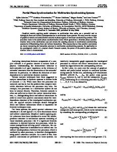
Fig. 1. Portion of the time series of z(t) = g(x(t)) = x1 (t)(x2 (t) + x5 (t)) we wish to estimate, function of the variables of the system (6).

and the respective Jacobians Dh(x) = (0, 0, 1, 0, 0, 0) DLf h(x) = (x3 , 0, x1 − b1 , 0, 0, 0) DL2f h(x) = (c1 + 2x3 (x1 − b1 ), −x3 , −x2 − 2x3

following six-dimensional system,   x˙ 1 = −x2 − x3 − x5      x˙ 2 = x1 + a1 x2 − x4 + (a1 − a2 )x5      x˙ = c + x (x − b ) 3 1 3 1 1  x˙ 4 = −x5 − x6 + x3       x˙ 5 = x4 + a2 x5    

− x5 + (x1 − b1 )2 , 0, −x3 , 0)

(8)

DL3f h(x) = (∗, a(x), ∗, 0, a(x), 0) DL4f h(x) = · · · (6)

x˙ 6 = c2 + x6 (x4 − b2 ) .

where a1 , b1 , c1 , a2 , b2 , c2 are real constants. The local observability condition described in the previous section can tell us whether there are parts of the dynamics that are unobservable using a specific output. Suppose we are given the output y = h(x) = x3 , consider the problem of estimation of the following signal z(t) = g(x(t)) = x1 (t)(x2 (t) + x5 (t)) through online measurements of y(t). A short segment of the time series of this variable that we wish to estimate, is given in Fig. 1. Numerical evidence shows that there are regions of the phase space from which the system (6) shows a bounded outcome, exponential divergence, or even escape to infinity (for negative x 3 or x6 ) in a finite time. We are unable to give a mathematical proof of boundedness of trajectories starting in an subset of the total phase space, therefore we assume boundedness of the trajectories in order to proceed with the discussion.

where a(x) = −[c1 + x3 (x1 − b1 )] − (x1 − b1 )x3 . We do not need to calculate Lie derivatives of the output higher than the third one to realize that the observability codistribution is of dimension at most three. Therefore, there must be a subset of the six equations of motion (6) (that evidently includes the output x3 ) that acts as a driving for the remaining part, so that the whole system (6) can be actually rewritten (at least locally) in a cascade form. It is now clear, from the calculation of DL 3f h(x) that the coordinate transformation that expresses the second variable x2 as x2 − x5 will make the system (6) appear in a cascade form. After all, the system (6) has been derived from coupling the two systems     z˙1 = −z2 − z3

z˙ = z + a z

2 1 1 2    z˙ = c + z (z − b ) 3 1 3 1 1

    z˙4 = −z5 − z6 + z3

z˙ = z + a z

5 4 2 5    z˙ = c + z (z − b ) . 6 2 6 4 2

(9)

that is composed by two coupled R¨ossler systems, via the linear change of coordinates z 2 → x2 + x5 , and that leaves all other coordinates unchanged. Clearly, the output y = x3 = z3 gives us no information on the driven subsystem of (9), hence neither the observability codistribution for (9), nor for (6) can be of full rank, since the systems (6) and

Partial Observers and Partial Synchronization 457

(ξ1 , ξ2 , ξ3 ) = (z1 , z2 , log z3 ) ,

η = log y

transforms the driving part of (9) in the form ˙ = Aξ(t) + g(η(t)) , ξ(t)

ξ(0) = ξ0

(10)

η(t) = Cξ(t)

10

5

e1(t)

(9) are linked by a smooth coordinate change, that preserves local observability. In principle, the Jacobians (8) give us enough information to build a local coordinate change that would transform system (6) into cascade form, to a form that (up to a coordinate transformation) is similar to (9), i.e. it has the same macroscopic properties, averaged quantities such as Lyapunov exponents, dimensions, concepts popular in the field of chaotic dynamics (in case this transformation is global, of course). In this case, we have the chance to estimate the quantity x1 (x2 +x5 ) from the system (6), from the output y = z3 , because we can construct an observer for the independent part of (9). As in [Nijmeijer & Mareels, 1997], the coordinate transformation



0

−5

−10

0

50

100 time

150




200







Fig. 2. Variable e1 (t) versus time for the error dynamics (12). The synchronization between the observer (11) and the system (10) provides us with an estimate of the variables (ξ1 , ξ2 , ξ3 ).

For the choice of the matrix K = (1 0 1) > , the variable e1 (t) is shown in Fig. 2. Assuming boundedness of the estimates ξˆ1 and ξˆ2 , the product ξˆ1 ξˆ2 is an estimate for g.

where 

ξ1 (t)





0

  d   ξ2 (t)  =  1    dt ξ3 (t) 1  

+ 



0

a1

    0   ξ2 (t) 

0

0

ξ1 (t)

5. Linear Error Dynamics



−1

The results presented in Sec. 2 show that conditions ensuring the existence of a solution to the posed problem are coordinate-free. At the same time, the methods for observer design developed so far are not so flexible. To illustrate this idea suppose for a moment that the drive system is represented by the following equations

ξ3 (t)

eξ3 (t) 0 −b1 + c1 e−ξ3 (t)

   

with output η(t) = (0 0 1)ξ(t). In this form, the pair (A, C) is observable, and a full observer with linear error dynamics can be constructed as ˙ˆ ˆ + g(η(t)) + K(ˆ ξ(t) = Aξ(t) η (t) − η(t)) , ˆ = ξˆ0 ξ(0)



0 . . . ξ˙ =  .  ..  0

1 ..

··· .. . .. .

.

··· ···

···







α1 (ξ1 )   ..     . ,  ξ +    ..    . 1   αn1 (ξ1 ) 0 0 ..   . 

y = ξ1

(11)

ˆ ηˆ(t) = C ξ(t) provided that is possible to find K such that the matrix A + KC is Hurwitz. Once variables (ξ 1 , ξ2 , ξ3 ) are estimated, it is possible to derive an estimate of x1 (x2 + x5 ) through a coordinate change. The ˆ − ξ(t), where e(t) = (e1 , e2 , e3 ) variable e(t) = ξ(t) provides the evolution of the error dynamics, given by e(t) ˙ = (A + KC)e(t) . (12)

(13) Then the system 

0 . . . ˙ˆ  ξ= .  ..  0

1 ..

.

··· ···

··· .. . .. . ···

+ K(ξ1 − ξˆ1 ),







α1 (ξ1 ) 0    .. ..       . .ˆ    ξ +  ..    . 1   αn1 (ξ1 ) 0 yˆ = ξˆ1

(14)

458 G. Santoboni et al.

is a partial observer for (1) with appropriate K in the sense that it ensures the following observation goal: ˆ kξ(t) − ξ(t)k → 0, as t → ∞ It is important to observe that in this case the error dynamics is linear. Thus one may pose the problem of finding conditions under which system (1) has a partial observer with a linear error dynamics. A solution to this problem can be derived similarly to [Nijmeijer & van der Schaft, 1990], following which we will look for the existence of a transformation s: Rn → Rn1 , s: x 7→ ξ such that in the new coordinates the ξ-subsystem takes the form (13) and hence admits the observer (14). Here we present the conditions of equivalence via state transformation of the systems (1) and (4) with the ξ-subsystem in the form (13): 1. Local observability of a part of variables dim dO(x) = n1 ∀ x ∈ Ω ⊂ Rn . 2. There is a vector field r on Ω ⊂ Rn that satisfies Lr h(x) = Lr Lf h(x) = · · · = Lr Lnf 1 −2 h(x) = 0 and

Lr Lnf 1 −1 (x) = 1

such that [r, adkf r] = 0 ∀ k = 1, 3, 5, . . . , 2n1 − 1 If, additionally, g = ψ ◦ s, and ξ is bounded, then ˆ is an estimate for the signal z. the signal ψ(ξ)

6. Conclusion In this paper we have considered an observer-based approach to study partial synchronization, a situation in which a synchronizing system can be built only for a subsystem of a given dynamical system. We used the existing theory of observability to define and apply a similar condition for partial observability. This theory applies when the observability condition (given a specific output) is not fulfilled. The partial observability condition enables us to build a partial observer, which allows us to estimate only the observable part of the dynamics, given a specific output. The theory we explained in this paper gives conditions needed to find partial observers for systems for which the standard observability condition

is not fulfilled. We have only described the basic conditions for its design, and after this, all standard techniques existing in control theory can be applied. Apart from the linearization of the error dynamics there are other systematic observer design procedures [Gauthier et al., 1992].

Acknowledgment G. Santoboni would like to acknowledge the Netherlands Organization for Scientific Research (NWO) for financial support.

References Afraimovich, V. S., Verichev, N. N. & Rabinovich, M. I. [1986] “Stochastic synchronization of oscillations in dissipative systems,” Radiophys. Quant. Electron. 29, 795–803. Blekhman, I. [1988] Synchronization in Science and Technology (ASME Press, NY). Fujisaka, H. & Yamada, T. [1983] “Stability theory of synchronized motion in coupled-oscillator systems I,” Prog. Theor. Phys. 69, 32–47. Gauthier, J., Hammouri, H. & Othman, S. [1992] “A simple observer for nonlinear systems, applications to bioreactors,” IEEE Trans. Automat. Contr. 37, 875–880. Huijgens, C. [1673] Horoloqium Oscillatorium (Parisis). Kailath, T. [1980] Linear Systems (Prentice Hall, Englewood Cliffs, NJ). Krener, A. J. & Respondek, W. [1983] “Nonlinear observers with linearizable error dynamics,” SIAM J. Contr. Opt. 23, 47–52. Landa, P. S. [1996] Nonlinear Oscillations and Waves (Kluwer, Dordrecht). Nijmeijer, H. & van der Schaft, A. [1990] Nonlinear Dynamical Control Systems (Springer-Verlag, NY). Nijmeijer, H. & Mareels, I. M. Y. [1997] “An observer looks at synchronization,” IEEE Trans. Circuits Syst. 44, 882–890. Pecora, L. M. & Carroll, T. L. [1990] “Synchronization in chaotic systems,” Phys. Rev. Lett. 64, 821–824. Pecora, L. M., Carroll, T. L., Johnson, G. A., Mar, D. J. & Heagy, J. F. [1997] “Fundamentals of synchronization in chaotic systems, concepts and applications,” Chaos 7, 520–543. Xia, X. H. & Gao, W. B. [1989] “Nonlinear observer design by observer error linearization,” SIAM J. Contr. Opt. 27, 199–216.