Partially Supervised Neighbor Embedding for Example-Based Image ...

Partially Supervised Neighbor Embedding for

Example-Based Image Super-Resolution IEEE Journal of Signal Processing, Vol. 5, No. 2, 2011 Kaibing Zhang, Xinbo Gao, Xuelong Li, and Dacheng Tao Presented by In-Yong Song

School of Electrical Engineering and Computer Science Kyungpook National Univ.

Abstract  Proposed

method

– Novel example-based image super-resolution reconstruction algorithm • Assumption for Textures – Containing multiple manifolds

• Use of clustering and supervised neighbor embedding(CSNE) – Class predictor for low-resolution(LR) patches » Use of unsupervised Gaussian mixture model – Estimating high-resolution(HR) patches » Use of supervised neighbor embedding » Utilizing class label information of each patch

2 / 30

Introduction  Existing

super-resolution approaches

– Interpolation-based method • Using base function or interpolation kernel function – Intuitional and highly efficient – Use of less additive information » Generating high resolution image of less perceptual version

– Degrading model-based method • Three step – Registration with a reference image, deblurring and fusion

• Use of a priori knowledge – Making SR reconstruction well-posed

3 / 30

• Tikhonov’s regularization – The most representative regularization based algorithms

• Farsiu et al. – Proposing bilateral total variation(BTV) operator

• Li et al. – Presenting locally adaptive bilateral total variation(LABTV) operator

• Problem of algorithms – Achieving good result » Under the limited imaging model and correct selection of regularization parameters – Difficult to practical application

4 / 30

– Example-based or learning-based method • Single-frame super-resolution method – Predicting high-frequency details of low-resolution

– Learning co-occurrence relationship between LR patches and their corresponding HR patches

• Freeman et al. – Modeling relationship between local regions of image and scenes by using Markov network » Sensitive to training examples

• Chang et al. – Assuming LR image and its corresonding HR image » Similar local geometry – Use of locally linear embedding » Estimating HR patch by minimizing reconstruction error and optimal weights – Problem of neighbor sizes 5 / 30

• Chan et al. – Use of histogram matching » Problem of neighbor embedding

• Extended Chan et al. – Considering edge and neighborhood sizes » Important role of reconstruction quality of HR – Treating edge patches and non-edge patches differently in neighbor size – Problem of algorithm » Highly depending edges detection » Selecting neighborhood size

– Proposed method • Novel example-based image super-resolution – Using clustering and partially supervised neighbor embedding(CSNE) algorithm – Use of Gaussian mixture model » Clustering LR patches into different categories to guide neighbor embedding

6 / 30

Review of neighbor embedding for super-resolution reconstruction  Neighbor

embedding for image super-resolution

– Brief formulation •

X s  {xsi }im1

: a training patches of low resolution images

•

Ys  {xsi }im1

: the corresponding high-resolution patches

•

X t  {xtj }mj 1 :

•

X t  {x }

j m t j 1

a set of low-resolution patches

: their corresponding high-resolution patches

• Three step – 1) Find k-nearest neighbors Nt j  {xtj (1) , xtj (2) ,..., xtj ( K ) } of each xtj

among all patches from X s , i.e., Nt j  X s . The distance i j measure matrix between xs and xt is defined as Dij , i  1,2,..., m, j  1,2,..., n.

The j th column of D is the distance

j between xt and all patches from X s

7 / 30

– 2) Compute weights ij which best reconstruct each xtj from j its neighbors N t

 j  min xtj 

 x

i ij s

(1)

xsi Nt j

where ij is the weights for xsi , subject to the following constraints:



ij

 1 and ij  0 if xsi  Nt j

xsi Nt j

j – 3) Compute each yt as follow:

ytj 



ij

ysi

(2)

xsi Nt j

• First, to find k -nearest neighbors of the input LR patch • Second, to compute optimal weights by minimizing

reconstruction error • Last, to compute a HR patch with linear combination of the HR patches corresponding to the k -nearest LR patches

8 / 30

Proposed algorithm  Describing

general idea of the proposed algorithm

– Framework of algorithm

Fig. 1. Illustration of neighbor embedding for image super-resolution.

9 / 30

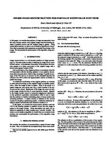
 Image

patches classification with Gaussian mixture model – Gaussian mixture model(GMM) • Set of parameters describing the mean and variation of the random vectors C p( xi |  * )   p( xi | c* )

(3)

c 1

* * * where c  ( c , c ,  c ) is the parameter set of the c th sub-calss. *

• The probability density function for random vectors 1 pxi |c ( xi | c, )  (2 ) D /2 *



*



xi

1 2

c

*  1   exp  ( xi  c* )T ( c ) 1 ( xi  c* )   2  here D represents the dimension of random vector xi

(4)

10 / 30

• The conditional probability C

pxi ( xi |  )   pxi |c ( xi | c, * ) c* *

c 1

• Thus, log of the probability of the N

C

i 1

c 1

(5)

X N  {xi }iN1

log pxi ( xi C , )   log  pxi |k ( xi | c, * ) c* *

(6)

• For the model parameters  * , a maximum of the fitness in terms of maximum likelihood(ML) ^

*  ML  arg max log px ( xi | C , * )

*

i

(7)

11 / 30

 Clustering

and supervised neighbor embedding for SR reconstruction – Partially supervised neighbor embedding for SR reconstruction • Taking account of the low-resolution patches containing multiple manifolds, corresponding to classes • Using class label information of input LR patches – Tuning the distance between samples in different classes » Embedding k -neighbors of the patches from the same class

12 / 30

– Algorithm • 1) The training samples X s are divided into using Gaussian mixture model • 2) Find k -nearest neighbors

among all patches from Dij

between

xsi and x tj

X s.

C

clusters by

Nt j  {xtj (1) , xtj (2) ,..., xtj ( K ) }

j of each xt

The distance measure matrix

is tuned as follows:

Dij'  Dij   max( D) M ij

i  1,2,..., m, j  1,2,..., n

(8)

i j where M ij  0 if xs and xt belong to the same class, otherwise 1.

• Supervised strength parameter  in(8) – Control of Using how much class information

» Finding k -nearest neighbors – Value range from [0, 1] » Calling partially supervised neighbor embedding within (0,1)

13 / 30

 Proposed

example-based image superresolution algorithm – Pseudo-code of proposed algorithm

14 / 30

• 1) Partition X t and X s into patches of size q x q with overlapping by one or two pixels • 2) Partition Ys into patches of size sq x sq with overlapping by s or 2s pixels accordingly, thus generating high-low training patch-pairs from X s , i.e., { ysi : xsi }im1; • 3) For all low-resolution patches {xsi }im1 , given initial cluster C , a class predictor (called CP) is learnt through unsupervised Gaussian mixture model. After CP constructed, all {xsi }im1 are divided into its corresponding class; • 4) For each patch xt In X t , find k -nearest neighbors among i m i j all {xs }i1, and the distance between xs and xt is computed as if CP(xsi , xtj )  1 then j

M ij  0

else

end if

M ij  1

Dij'  Dij   max( D) M ij

i  1,2,..., m, j  1,2,..., n 15 / 30

• 5) Compute the optimal weights W j by minimizing the error j of reconstruction for xt ; • 6) Compute the high-resolution patch to be estimated from the weights sum of W j with the k patches in Ys corresponding to the k -nearest neighbors found in X s ; • 7) Merge all

ytj

s to obtain

ytj

Yt

16 / 30

 Computational

complexity

– Considering each step of algorithm 1 •

m and n

: the number of patches in the training set and the input image

• q 2 : the size of each LR patch •

C

: the number of clusters of the Gaussian mixture model

• k : the number of neighbors Table I. Computational complexity of the proposed algorithm in each step

17 / 30

Experimental results and evaluations  Training

and testing images

– Six images • Including human, plants and animals

Fig. 2. Training images. From left to right, top to bottom are labeled No.1 to No. 6. 18 / 30

– Getting input LR images • Degrading by averaging blurring operation – within 4 x 4 neighbors

• Down-sampling with factor 4 – product a testing input image

Fig. 3. Input LR images.

19 / 30

 Experimental

results

– Comparing performance of the CSNE with SRNE and NeedFS • 3 x 3 size of low-resolution patches – Two pixels overlapped between adjacent patches

• 12 x 12 size of high-resolution patches – Eight pixels overlapped between adjacent patches

• Parameter  – Set up as 0.1

2552 PSNR  10log10 MSE

(9)

20 / 30

• Objective assessment – Use of peak-signal-to-noise ratio(PSNR) 2552 PSNR  10log10 MSE

(9)

Table II. Performance of PSNR (dB) using different algorithms

21 / 30

– Resulting image • No. 1

Fig. 4. 4X recovery of No. 1 using different methods. From left to right, top to bottom: the low resolution image; the original image; Bicubic; SRNE; NeedFs; the proposed method.

Fig. 5. Local magnification of No. 1. From left to right: the original image; Bicubic; SRNE; NeedFs; the proposed method. 22 / 30

• No. 4

Fig. 6. 4X recovery of No. 4 using different methods. From left to right, top to bottom: the low resolution image; the original image; Bicubic; SRNE; NeedFs; the proposed method.

Fig. 7. Local magnification of No. 4. From left to right: the original image; Bicubic; SRNE; NeedFs; the proposed method. 23 / 30

• No. 6

Fig. 8. 4X recovery of No. 5 using different methods. From left to right, top to bottom: the low resolution image; the original image; Bicubic; SRNE; NeedFs; the proposed method.

Fig. 9. Local magnification of No. 1. From left to right: the original image; Bicubic; SRNE; NeedFs; the proposed method. 24 / 30

 Part

clustering results and the weight of neighbor patches changed based on cluster information – Demonstrating clustering results • Effect on the weight of neighbor patches for reconstruction Table III. Number of patches of each cluster of the No. 3 Training set.

25 / 30

Fig. 10. Part of clustering results for LR patches in the No. 3 training set.

26 / 30

– Showing how the weight of neighbor patches changed • Based on clustering information Table IV. Comparison of weights of neighbor patches between SRNE (five neighbors) and the proposed algorithm (ten neighbors) for the 2000th patch

Table V. Comparison of weights of neighbor patches between SRNE (five neighbors) and the proposed algorithm (ten neighbors) for the 3000th patch

27 / 30

 Effect

of supervised strength parameter

– Affecting how much class-information for neighbor embedding • If   0 , no any class information of patches used – Equivalent to the algorithm SRNE

• If   1 , a fully supervised neighbor embedding

Fig. 11. Performance of PSNR versus different number of neighbors for NO. 3. The supervised strength alpha ranges from 0 to 0.3.

Fig. 12. Performance of PSNR versus different number of neighbors for NO. 3. The supervised strength alpha ranges from 0.4 to 1.0. 28 / 30

Fig. 13. Performance of PSNR versus different number of neighbors for NO. 6. The supervised strength alpha ranges from 0 to 0.4.

Fig. 14. Performance of PSNR versus different number of neighbors for NO. 6. The supervised strength alpha ranges from 0.5 to 1.0. 29 / 30

Conclusions  Proposed

method

– Novel example-based image super-resolution reconstruction algorithm • Use of clustering and supervised neighbor embedding(CSNE) – Use of unsupervised Gaussian mixture model » Class predictor for low-resolution(LR) patches – Utilizing class label information of each patch – Use of supervised neighbor embedding

» Estimating high-resolution(HR) patches

– Experiment of proposed method • Evaluating proposed algorithm

30 / 30

– An Improved Super-Resolution with Manifold Learning and Histogram Matching

31 / 30

– Locally Linear Embedding

32 / 30

– Two key setps • 1. Find weight matrix W of linear coefficients: Enforce sum-to-one constraint with the Lagrange Multiplier:

• 2. Find projected vectors Y to minimize reconstruction error must solve for whole dataset simultaneously

We add constraints to prevent multiple/degenerate solutions:

cost function becomes: the optimal embedded coordinates are given by bottom m+1 33 / 30 eigenvectors of the marix M