positioning and tracking (PTV) of particles, dispersed either on the free surface or in the flow ... for which traditional PTV algorithms have shown their limitations.
PARTICLE-BASED IMAGING METHODS FOR THE CHARACTERISATION OF COMPLEX FLUID FLOWS D. Douxchamps1, B. Spinewine2,3, H. Capart4, Y. Zech2 and B. Macq1 1
Comm and Remote Sens Lab, Université catholique de Louvain, Belgium. 2 Dept. of Civ and Env Eng, Université catholique de Louvain, Belgium. 3 Fonds pour la Recherche dans l’Industrie et l’Agriculture, Belgium. 4 Dept of Civil Engineering, National Taiwan University, Taiwan.
ABSTRACT We review a set of particle-based imaging methods, so-called the Voronoï methods, for the three-dimensional characterisation of fluid-granular flows. The methods mainly involve positioning and tracking (PTV) of particles, dispersed either on the free surface or in the flow itself, in order to estimate local flow velocities and/or surface topography. Detection of particle centroids on digital images, stereoscopic reconstruction of 3D particle positions, and tracking on successive frames, form the core sections of the paper. The originality of the methods is to rely on the geometrical properties of the Voronoï diagram to perform stereo reconstruction and tracking even for the case of very dense and fluctuating dispersions, cases for which traditional PTV algorithms have shown their limitations. The capabilities and robustness of the methods are qualitatively illustrated on a wide range of 2D and 3D applications. 1 INTRODUCTION The use of digital imaging for qualitative and quantitative characterisation of fluid flows is not new. In recent years however, with the rapid development of powerful digital cameras at affordable prices and the advances in robust and fast image processing techniques, this tool has become very popular. The present paper focuses on the potential of a set of methods, socalled Voronoï imaging methods and aimed at characterising fluid-granular flows through robust particle positioning and tracking algorithms. Fluid-granular flows involve the movement of a fluid and/or a set of particles. Such flows of disperse phases are encountered in a wide variety of situations of scientific and engineering interest. Particulate flows include liquid-entrained gas bubbles, aerosols, dry granular flows, fluidised beds of particles, and liquid-saturated particulate currents. Purely fluid flows, on the other hand, may often be visualised by diluting seeding particles that act as tracers of the flow field, either within the fluid itself (neutrally buoyant particles) or at the free surface, if any (floaters). A typical set-up is as presented in Fig. 1: a flow seeded with particles is imaged from above or through a transparent side-wall. The particles are roughly identical and appear brighter than the surrounding fluid on the digital images. The flow is imaged from a single camera (Fig. 1a) or from two cameras in a stereoscopic arrangement (Fig. 1b).
1
2 3 (a)
(b)
(c)
Figure 1. Typical measurement set-up of a flow of particles imaged through a side-wall, using: (a) a single camera; (b) two cameras in a stereoscopic arrangement. (1) side-wall; (2) digital camera; (3) lighting system. (c) sample images in a stereoscopic arrangement.
In most of these situations, the individual elements of the disperse phase (bubbles, grains or tracers) can be approximated as rigid bodies undergoing distinct motions. The dynamic system can thus be abstracted into an evolving configuration of particle positions. The sought measurements include 2D and/or 3D positioning of the visible grains, tracking of 2D and/or 3D particle motions, and reconstruction of full sets of particle trajectories. The approach presented here follows the work of Capart et al. (2002) and Spinewine et al. (2003). The core of the proposed methods consists in exploiting the special properties of Voronoï diagrams (Ahuja 1982; Okabe et al. 1992). These define spatial tessellations of the 2D plane or 3D space into cells centred around individual feature-points (see section 2.2.2). After abstraction of digital images into discrete sets of particle positions, the Voronoï diagram is used for every main step of the analysis: 1) the 2D tessellation is invoked to speed up the stereoscopic matching of particles; 2) the diagram furnishes special patterns, or templates, which allow tracking of particle neighbourhoods in time. A brief presentation of these methods constitutes the central section of the present paper: section 2 is devoted to particle positioning in 2D and 3D; section 3 describes the Voronoï particle tracking algorithm. Ultimately, the capabilities of the methods are illustrated in section 4 through a range of applications. 2 PARTICLE POSITIONING 2.1 Detection and 2D positioning The first step of the analysis consists in the localisation of particle centroids on individual images. For each instant at which an image is acquired, one seeks to identify the set of particle image positions {Ri}, where Ri = [Xi Yi]T is the 2D position of the i-th particle (with superscript T designating the matrix transpose). Particle images show up on the acquired frames as white blobs of a certain size against a dark, relatively noisy background (see Fig. 2a). An image neighbourhood associated with a particle can be approximated by a Gaussian grey-level function centred on the particle centroid, with a diameter D that scales with the pixel diameter of the particles. Such bell-like regions are first highlighted by convoluting the image with a Laplacian-of-Gaussian (Mexican hat) filter of width D (Jähne 1995). This effectively suppresses high frequency noise and low frequency variations in illumination (Fig. 2b, c). Local maxima of the highlighted images are then sought. This is
done by a "dish-clearing" iterative algorithm: a global maximum is found, then a Gaussian bell of diameter D is subtracted from the neighbourhood grey level values; a new global maximum is found, and so on. The position of each maximum is finally refined to subpixel accuracy by way of a second-degree interpolation surface fitted around the discrete pixel position. These various steps are shown in Fig. 2, with details given in Capart et al. (2002). The expected root-mean-square accuracy on the X and Y image co-ordinates obtained with such a procedure is of the order of 0.25 pixel (Veber et al. 1997).
(a)
(b)
(c)
(d)
Figure 2. Particle identification procedure: (a) image fragment; (b) image (a) after low pass filtering; (c) image (b) after high pass filtering; (d) particle positions at brightness maxima of (c).
2.2 Stereo reconstruction and 3D positioning When two sets of synchronised stereoscopic images are acquired from two different viewpoints A and B, one may try to relate the sets of particle image positions {Ri(A)} and {Rj(B)} to the set of actual particle positions {ri} in 3D space. Two difficulties arise when doing that: the first is the problem of 3D reconstruction of a single particle based on its images under two viewpoints; the second, which comes when the number of visible particles on the images is large, is the problem of correspondence: find which particle on one image corresponds to which one on the other image, or in other words which pairs of particle images should be used in the 3D reconstruction process. 2.2.1 Stereo reconstruction Referring to Fig. 3, the first problem aims to find a transformation that relates the set of 2D images co-ordinates of any point P to its world co-ordinates. We suppose that the cameras at viewpoints A and B are calibrated. A wide range of methods exist to perform camera calibration but their description goes beyond the scope of the present paper. The reader can refer to Trucco and Verri (1998), Jain et al. (1995), Tsai (1987), and Faugeras (1999) for examples of simple calibration methods. As illustrated in Fig. 3, in the remainder one will assume that the image formation can be modelled as an affine transformation, i.e. a central projection from a virtual camera focal point (A, B) onto the image plane (Φ, Ψ). One can then easily compute the 3D projection line (or ray) associated to each image pixel as the line passing through the focal point of the camera and the pixel location on the image plane. Defining rP = [xP yP zP]T as the world co-ordinates of point P (Fig. 3), and RP(A) = [XP(A) YP(A)]T as the 2D image co-ordinates of P, associated with the camera viewpoint A (P' in left image plane Φ), one can obtain image co-ordinates from known world co-ordinates through
α [X(A) Y(A) 1]T = [A(A)] [x y z]T + b(A)
(1)
where α is a scalar coefficient and matrix [A(A)] and vector b(A) are obtained from the calibration procedure. Conversely, a point P having its projection P' with image co-ordinates RP(A) = [XP(A) YP(A)]T in plane Φ under viewpoint A is known to belong to the ray AP (or AP' as seen on Fig. 3) defined by parametric equation rAP(α) = rA + α sAP ,
(2)
where vectors rA and sAP are given by rA = -[A(A)]-1 b(A) ,
sAP = [A(A)]-1 [XP(A) YP (A) 1]T.
(3a,b)
If the same procedure is applied to viewpoint B, and using the rays AP' and BP" associated to the matched pixels co-ordinates of one and the same particle P in images A and B, the reconstructed 3D position of the particle can be estimated as the intersection of these two rays. However, due to inaccuracies in the calibration and detection processes, the two rays will generally not intersect (inset in Fig. 3), but pass close by. The midpoint of the segment MN corresponding to the least distance between the two rays constitutes an approximation of the true particle position rP : l = ( [rN - rM]T [rN - rM] )½ .
rP = ½ [rM + rN] ,
(4a,b)
l is the length of the segment MN and constitutes a kind of criterion of quality of the approximation. It will prove useful in the next sub-section when trying to perform the 3D reconstruction process in the presence of a large number of particles.
P
N M
P
A
B
Figure 3. Imaging geometry: physical point P and its image projections P' and P'' on the two stereo views. Rays emanate from focal points A and B of the two central projections. The trace of the epipolar plane comprising P is shown in dashed lines. Inset : due to imperfections in the imaging geometry, the two rays may not perfectly intersect.
2.2.2 Correspondence problem When the number of particle images on both views is large, we first need to solve the correspondence problem, i.e. finding which particle on one view corresponds to which one on the other view, or which pairs of rays should be made to intersect. While classical 3D reconstruction involves matching properties of an image point (like texture), particle-based imaging techniques can only rely on geometrical relations based on particle positions since all particles are identical. Suppose that the only available information about a particle P is the position RP(A) of its image P' on the left view (plane Φ), and that one wishes to find RP(B). Neglecting imperfections of the imaging geometry, physical point P is known to belong to the plane ABP', called the epipolar plane (see Fig. 3). Its intersection with the right image plane is a straight line εε whose parametric equation can be derived from the calibration matrices and from the image co-ordinates of P'. The straight line εε, called the epipolar line, constitutes the locus of all possible projections, in the right image plane, of a physical point having projection RP(A) in the left image plane (P' on Φ). The true projection RP(B) (P" on Ψ) is known to lie along this line or, due to inevitable imperfections of the imaging process, to fall somewhere close to the epipolar line. Instead of considering all particles on the right image as possible candidates for correspondence, an efficient solution for correspondence will restrict the set of candidates to particles located close to the epipolar line. We proposed (Spinewine et al., 2003) a global optimisation procedure, by resorting to the geometrical properties of the Voronoï diagram to speed up repeated searches of neighbouring points to the epipolar line.
sk Vi
Vi Pi
(a)
Si
Pi
(b)
vk
(c)
Figure 4. 2D and 3D Voronoï diagrams: (a) planar Voronoï diagram Vi (thick lines); (b) Voronoï vertex star Si (thick lines) surrounding Pi, discussed in more details in section 3; (c) a 3D Voronoï cell vk around point pk .
The Voronoï diagram (Fig. 4) is a geometrical construction which divides the space into a set of polytopes, or cells, surrounding each feature point. Each Voronoï cell Vi (in 2D) or vi (in 3D) encompasses the region which lies closer to Ri (respectively ri) than to any other featurepoint of the set. The construction presents many useful properties, discussed in a general context in Okabe et al. (1992). In particular, the diagram organizes the dispersion of points into a network of neighbourhood relations which can be used to speed up nearest-neighbour
queries (Preparata and Shamos 1985), a property very useful in the present context to accelerate the stereoscopic matching step. It would be very tempting to believe that, among the various candidates for correspondence along the epipolar line, the true projection P" will automatically be the one for which the residual distance between the corresponding two rays emanating from both focal points is minimised, i.e. making the two rays almost exactly intersect. However, this minimization is ill-conditioned in the case of very dense particle distributions: since all candidates have been chosen close to the epipolar line, their ray will thus, by construction, pass close to the ray associated to the point in image A. Thus, performing correspondence sequentially for each particle on image A taken one by one, may lead to mismatches. In order to obtain satisfactory results but keep using the minimal ray distance criterion, we used a global approach on the whole set of particles. A global ‘distance’ match matrix is built, with non-zero values corresponding to ray discrepancies for every pair of match candidates. The distance matrix is further simplified by limiting the candidate search to the part of the epipolar line that corresponds to the considered depth range of analysis, making it very sparse. Finding a solution then constitutes a standard bipartite graph optimisation problem, for which an efficient solution can be found using the Vogel algorithm. It consists in considering for each ray the best match and the second best match, then constructing a reasonable global optimum by picking ray pairs in the order of maximum difference between first and second best choices. We refer to Spinewine et al. (2003) for details. Other useful properties of the Voronoï diagram will be exploited below for obtaining flow velocities from particle displacements between successive frames. Figure 5 gives an example of reconstructed 3D positions from two stereo views of a dense fluidised bed of particles imaged through a sidewall.
(a)
(b)
(c)
Figure 5. Result of stereoscopic matching procedure. (a) typical dispersion of near-wall particles as seen from the left view (right view is not represented); (b) reconstructed 3D positions of the particles. Grey levels are assigned according to depth, bright for near-wall particles, darker for deeper ones; (c) side view of (b), solid line indicating wall position.
2.2.3 Refraction effects When the imaged scene is immersed in a liquid and seen from the outside through a transparent wall, as is often the case for fluid applications, the image formation can be strongly influenced by refraction effects. Each interface separating materials of different refraction indexes will bend light rays according to Snell's law. In general, these effects will
not preserve the affine character of the image formation, and must be faced using some form of inverse ray tracing. However, the affine character of the projection can be preserved to a very good approximation in the simple case of a liquid-bathed scene observed through a plane wall, and under some restrictions relative to imaging configuration. This is demonstrated in an internal report (Capart 2000), where quantitative estimates of the quality of the approximation are also given. The operations outlined above can then be performed with no changes, with the restriction that the camera calibration step must be performed with a target placed in refraction conditions identical to those of the actual experiments: whereas the affine character of the projection is approximately preserved, the parameters of the projection are not; the apparent position of the focal point, in particular, is influenced strongly by the heterogeneous character of the transparent medium. 3 PARTICLE VELOCIMETRY Besides particle positions, information of particular interest for fluid applications is the particle velocities. Those are obtained as inter-frame displacements from the particle positions derived using the reconstruction methods from the previous section. This class of methods is referred to as Particle Tracking Velocimetry (PTV), as opposed to Particle Image Velocimetry (PIV) where average velocity vectors are obtained for a cloud of particles based on image cross-correlation techniques. The advantage of PTV over PIV is that individual particle motions are resolved, and that full sets of particle trajectories can be reconstructed by following one and the same particle over many successive frames, information that might be crucial for granular flow applications or fluid applications involving small-scale features (vortices, turbulence), for which Lagrangian information is needed. Whereas the application of traditional PTV algorithms (minimum displacement, path coherence, …) is restricted to relatively coherent flows with diluted particle tracers, Capart et al. (2002) have proposed a more robust set of methods that allow to reconstruct full sets of particle trajectories even in extreme conditions as for very dense, intensively sheared dispersions. As for the 3D reconstruction method discussed above, the geometrical properties of the Voronoï diagram are used to track particle neighbourhoods from frame to frame. Those pattern-based Voronoï methods were extended to the third dimension by resorting to stereoscopic imaging. We now briefly summarize the principle of the methods, and refer the interested reader to the two detail papers for in-depth presentations, applications and comparisons with alternative approaches. Sets of 2D or 3D particle positions at successive times have first been acquired by repeated application of the above positioning methods to each frame of a movie sequence. Let {r i, m} and {r j, m+1} be two such sets of particle positions sampled at successive times t m and t m+1 = t m + ∆t . Particle velocities vi (t m+1/2) can be estimated by expression v i , m +1 2 =
r j ( i ), m +1 − r i , m
, (5) ∆t provided one can first "connect the dots" and establish a pairing j(i) between positions r i, m and r j(i), m+1 belonging to one and the same physical particle. When dealing with a moving dispersion of many identical particles, the main problem consists in establishing this correspondence: finding which particle on one snapshot corresponds to which one on the next. The particle tracking problem can thus be seen as a time-domain variant of the stereo matching problem addressed previously.
For dilute particle dispersions or slow motion, the correspondence problem can easily be solved simply by pairing together the particles on one frame and the next which are nearest to each other (see e.g. Guler et al. 1999). For dense dispersions or rapid motion, however, legitimate pairing candidates may travel further away on successive frames and the minimum displacement criterion breaks down. An alternative approach derives from the following observation: while individual particles are identical to each other, the local arrangements that they form with their neighbours are unique and may be preserved by the flow long enough to serve as basis for tracking. Particle pairing can then be performed based on pattern similarity. We again resorted to the Voronoï diagram to implement such pattern-based tracking. Nearby particles are paired according to the geometrical similarity of their Voronoï cells. This similarity is estimated as follows: "stars" are first constructed by connecting a given particle centre to its Voronoï neighbours (i.e. the particles with which it shares a cell face), as illustrated on Figs. 4b and 4c for both the 2D and 3D cases. The stars belonging to two pairing candidates can then be compared based on a distance measure, defined by making their centres coincide and measuring the distances between the star extremities. Once these indicators are available for all possible pair candidates, a global optimum problem can be defined and solved that maximizes the "goodness-of-fit" of matched particles. For two dimensions, the overall method is illustrated on Fig. 6 for a plane granular flow. While graphical representation is harder in 3D, the algorithms themselves generalize straightforwardly to the third dimension.
(a)
(b)
(c)
Figure 6. Pattern-based velocimetric tracking: (a) original image fragment and particle positions; (b) Voronoï diagrams built on sets of particle positions at two successive time instants; (c) velocity vectors built by matching of the local Voronoï patterns. (Note: the 2D algorithm is illustrated here, but the methods generalise straightforwardly to 3D.)
4 APPLICATIONS A series of applications in fluid-granular flows is now presented, showing some of the capabilities of the Voronoï imaging methods. They refer mainly to open-channel applications, which are the research fields of the authors. The first involves the 3D reconstruction of the free surface topography in the case of a transient dam-break wave passing through a sudden enlargement. The second is a fluid-granular application that investigates the movement of an erodible sediment bed set in motion by a similar dam-break wave. The third aims at reconstructing the evolution of the free surface of the flow over a train of antidunes, and compares stereoscopic measurements with a monocular approach that derives local flow depth from free surface velocity. The fourth is a true 3D-in-volume application, characterising the vortices produced during the filling phase of a lock chamber in a scale model of the lock of Lanaye, the largest inland-navigation lock in the world in terms of volume of water, that will
be built near Liège in Belgium. The last application tracks the 3D movements of the particles constituting a dense fluidised bed reproduced in a small cylindrical fluidisation cell. 4.1 Dam-break wave through a sudden enlargement The first application concerns the propagation of an idealised dam-break wave in a channel with a sudden enlargement. A sudden wave of water is created in a narrow channel by rapidly raising a gate separating a body of water initially at rest in the upstream reach from the downstream channel. Some 80 cm downstream of the gate, the channel suddenly widens from 12 cm to 50 cm. The wave spreads out in the wider reach, then reflects against the opposite side-wall and progressively forms an oblique hydraulic jump downstream (Fig. 7).
(a)
(b)
(c)
Figure 7. Three snapshots of the propagation of a dam-break wave in a channel with a sudden enlargement. (a) the initial lobe of propagation is clearly visible when the wave invades the wider reach; (b) - (c) at later instants reflection bores form on the opposite side-walls.
(a)
(b)
(c) Figure 8. Imaging results for the dam-break wave through a sudden enlargement: (a) 3D free surface topography derived from 3D positions of floating tracers; (b) average velocity map at time t = 2.75 s. after dam-break initiation; (c) particle trajectories tracked over a long period in permanent flow conditions, showing the re-circulation zone and the oblique hydraulic jump.
The flow was seeded with small white wooden floaters at its free surface, both in the upstream water body and in the downstream dry region. The 3D positions and movements of those floaters were tracked using two synchronised fast CCD cameras operating at 200 frames per second, positioned in a stereoscopic arrangement above the channel. 3D positions allowed to derive the free surface topography, as shown in Fig. 8a. Tracking of particle motions delivered average velocity fields, as shown in Fig. 8b at time t = 2.75 s after gate opening. Longer particle trajectories were obtained in permanent flow conditions, and are shown in Fig. 8c; several experiments were performed with the cameras placed above distinct viewing regions, and the results could be merged together due to the high reproducibility of the tests. Details of those experiments are found in Soares Frazão et al. (2003). 4.2 Plane dam-break wave over a movable bed The second application consists in the propagation of a dam-break wave in a prismatic channel with fixed side-walls but a movable bed, made of light PVC pellets. The erosive force of the wave sets the underlying sediment bed in motion, and the particles join the flow to form a mixture of water and grains in suspension. A bore forms at the forefront of the wave, that propagates downstream and continues to pick up sediments from the bed. The flow was imaged laterally using two fast CCD cameras put aside each other and covering contiguous regions. The experimental set-up is sketched in Fig. 9, along with a snapshot of the flow moments after opening the gate. Again, several tests were performed at different positions and the results were merged together to produce mosaic images of the flow over a wider region. Here, the challenging aspect is the tracking of all the particles constituting the bed. The very dense concentration of particles associated with fast movements constitutes a critical test for particle tracking algorithms, but the pattern-based Voronoï method proved robust. Mosaic images and tracking results are presented in Fig. 10 at times t = 0.25 s and t = 0.75 s after gate opening. A detailed presentation of the experiments will be found in Spinewine and Zech (2002). 4
5
2
3
1
(a)
(b)
Figure 9. Propagation of a dam-break wave over a movable sediment bed: (a) experimental set-up showing (1) channel, (2) gate, (3) cameras, (4) lighting, (5) diffusive back-lighting; (b) snapshot of the flow moments after the gate is raised.
(a)
(b)
a (c)
(d)
c (e)
Figure 10. (a)-(b)-(d) image mosaics of the flow at times t = 0, 0.25 and 0.75 s after gate opening; (c)-(e) particle velocities and flow interfaces tracked at times t = 0.25 and 0.75 s after opening.
4.3 Open channel flow over a train of antidunes Antidunes is a class of fluvial bedforms that appear when rapid, shallow currents propagate over coarse granular material, and is characterised by in-phase coupling between the oscillatory sediment bed and the flow free-surface (Kennedy 1963, Allen 1984). Among other features, antidunes are notable for the fact that they vanish rapidly once the flow wanes. As a result, they leave few lasting traces aside from bedding and grain-sorting effects and their geometry, in particular, has to be studied when the flow is active. For this experiment, two completely different methods were simultaneously used: a velocimetric technique and a stereoscopic technique, both analysing a dispersion of particles on the flow surface. The velocimetric technique used a high-speed camera and the Voronoï tracking algorithms described above to acquire the velocity field. One can show that it is possible to derive the surface elevation from the velocity field for this particular class of flows (Douxchamps et al. 2000) using the Bernoulli equation which take the following simplified form:
η =η −
u (u −u ) g
(6)
where η is the surface elevation, u is the particle velocity, g is the gravity and the overline denotes the mean over a streamline. The stereo analysis simultaneously directly captured the 3D position of the tracers to reconstruct the surface shown in Fig. 11a. Figure 11b compares cross-sections of the surfaces reconstructed by both methods. The good correlation of both surfaces show the adequacy of the methods.
(a)
(b)
Figure 11. Flow over a train of antidunes. (a) Water surface reconstructed by stereo; (b) a comparison of the two methods for several sections of the surface along the x axis
4.4 3D vortices induced during the filling phase of a navigation lock Planning the construction of the largest inland-navigation lock in the world at Lanaye, Belgium, a scale model of a bottom injector has been designed at the Laboratoire de Recherches Hydrauliques of the Ministry of Equipment and Transport in Châtelet, Belgium, in order to investigate the flow movements induced within the lock during its filling phase. The scale model is represented in Fig. 12a. Filling of the lock is governed by bottom injectors, one of them is represented in the central part of the scale model at the bottom-left corner of the figure.
(a)
(b)
Figure 12. Tracking of 3D vortices within the scale model of a navigation lock during filling phase. (a) photograph showing the model, the bottom injector in the central part at the lower-left corner, and the position of the two cameras; (b) reconstructed particle trajectories showing the ascending vortical structures developing in the corner opposite the cameras.
Visual inspection of the flow was possible through the transparent side-walls, and two synchronised fast CCD cameras were placed in a stereoscopic arrangement as visible in Fig. 12a. The cameras tracked the movements of small white particles dispersed in the model before initiation of the experiment. The particles are almost neutrally buoyant (with a relative density s = 1.048) and were supposed to be entrained by the flow with negligible drag. During the filling phase, the incoming jet from the injector reflects against the opposite wall and creates ascending vortical structures in the corners. The swirling movements of the particles could be tracked in 3D using the two cameras, as seen on Fig. 12b, where one can see that the vortex axis bends towards the centre of the model as it moves upwards. A key challenge of that application was to account for strong refraction effects at the air/glass/water interfaces, through a precise camera calibration. Details of the experiments are found in the B Eng thesis of de Backer (2001). 4.5 Fluidised bed The last application concerns stereo fluidisation cell experiments. Fluidised beds are encountered in a wide variety of industrial processes involving chemical reactions, exchanges between distinct phases and mixing. The principle of the tests is as follows. Subject to an ascending water current, a layer of loosely packed grains expands into a fluidised suspension. The concentration adapts to the water flux until the mean drag balances the submerged weight of the grains. In this fluidised state, the suspended particles undergo weakly correlated fluctuating motions, exploring a variety of spatial arrangements. Different particle concentrations and mean energies of the fluctuations can be explored by simply tuning the fluid flow. The device is presented in Fig. 13. Tests were carried out in a cylindrical fluidisation cell with a small plane observation window fitted to the cell wall to allow visual access without optical distortion. The particles were light spheres with a diameter d = 6 mm.
6
4 (a)
3
5
2 1 (b)
(c)
Figure 13. Fluidisation cell experiments. (a) – (b) The fluidisation cell : 1) bounding plates, 2) Perspex cell shaft, 3) impermeable joints and fixation screws, 4) incoming water flow, 5) layer of lead spheres to diffuse water current, 6) fluidised bed. (c) Example of granular trajectories of visible particles obtained for a fluidisation cell experiment at a bulk concentration of 38 %: top view and 3D view.
Two synchronised CCD cameras were used to obtain stereo image sequences and track particle movements in 3D. Occlusion, however, prevented optical penetration deeper than a few particle diameters. Examples of fluctuating granular trajectories obtained for a fluidisation cell experiment at a bulk concentration of 38 % are illustrated in Fig. 14 under different viewpoints. The key component here is the stereoscopic positioning step. Reliable 3D positions must be measured in order to record continuous trajectories. A more detailed description of those fluidisation cell tests is given in Spinewine et al. (2000). 5 CONCLUSIONS We presented and illustrated a set of particle-based imaging methods for the threedimensional characterisation of fluid-granular flows. After abstraction of the digital images into discrete set of particle positions, the methods, so-called the Voronoï methods, rely on the geometrical properties of the Voronoï diagram to perform stereoscopic matching between synchronised pairs of stereo views, and tracking (time-matching) of particles between successive images. The PTV algorithm is especially robust in the case of dense and highly fluctuating dispersions of identical particles, and are therefore suitable for flow characterisation in extreme conditions. The capabilities and robustness of the methods have been illustrated with a range of 2D and 3D flow applications, including highly transient water flows with tracers, granular flows and fluidised beds. ACKNOWLEDGMENTS The authors members of the Dept of Civ and Env Eng at the Université catholique de Louvain wish to acknowledge the financial support offered by the European Commission for the IMPACT project under the fifth framework programme (1998-2002), Environment and Sustainable Development thematic programme, for which Karen Fabbri was the EC Project Officer. In addition, the second author wishes to acknowledge the Fonds pour la Recherche dans l’Industrie et l’Agriculture, Belgium, for his support through a PhD fellowship. The laboratoire de Recherches Hydrauliques at Châtelet, Belgium, is gratefully acknowledged for inviting and helping the second author to perform the experiments on their scale model of the navigation lock of Lanaye. REFERENCES Ahuja N (1982) Dot pattern processing using Voronoï neighborhoods. IEEE PAMI 4: 336-343. Capart H; Young DL; Zech Y (2002) Voronoï imaging methods for the measurement of granular flows. Exp Fluids 32:121-135. Capart H (2000) refract: refraction effects in stereo viewing. Geomorfica technical note, March 2000 De Backer A (2001) Développement et application de techniques d'imagerie digitale pour l'analyse tridimensionnelle d'un écoulement complexe. BEng thesis, Haute école Leonardo da Vinci (ECAM), Belgium (in French).
Douxchamps D; Devriendt D; Capart H; Craeye C; Macq B; Y.Zech (2000) Three-dimensional reconstruction of the oscillatory free-surfaces of a flow over antidunes: stereoscopipc and velocimetric techniques, Proc of the IEEE Oceans 2000 Conf., Providence, RI, USA. Faugeras O (1999) Three-dimensional computer vision: a geometric viewpoint. MIT Press. Guler M; Edil TB; Bosscher PJ (1999) Measurement of particle movement in granular soils using image analysis. J Comp Civ Eng 13: 116-122. Jähne B (1995) Digital image processing. Springer. Jain R; Kasturi R; Schunck BG (1995) Machine vision. McGraw-Hill. Kennedy JF (1963) The mechanics of dunes and antidunes in erodible-bed channels, Journal of Fluid Mechanics, Vol.16, 1963, pp 521-544 Allen JRL (1984) Sedimentary structures - their character and physical basis, Amsterdam: Elsevier. Okabe A; Boots B; Sugihara K (1992) Spatial Tessellations: Concepts and Applications of Voronoï Diagrams. Wiley. Preparata FP; Shamos MI (1985) Computational Geometry: An Introduction. Springer. Soares Frazão S; Lories D; Taminiau S; Zech Y (2003) Dam-break flow in a channel with a sudden enlargement. Accepted for publication at the XXX IAHR Congress, Thessaloniki, Greece, 25-31 August 2003. Spinewine B; Capart H; Larcher M; Zech Y (2003) Three-dimensional Voronoï imaging methods for the measurement of near-wall particulate flows. Exp Fluids. In press. Spinewine B; Zech Y (2002) Dam-break waves over movable beds: a “flat bed” test case. Proceedings of the second international workshop of the IMPACT project, Mo-i-Rana, Norway, 16-17 September 2002. CD-Rom proceedings. In press. Spinewine B; Capart H; Zech Y (2000) Stereoscopic imaging measurements of solid concentrations in dense granular flows. 10th Int. Conf. on Transport & Sedimentation of Solid Particles, Wroclaw, Poland, September 2000, pp. 497-509. Trucco E; Verri A (1998) Introductory techniques for 3-D computer vision. Prentice Hall. Tsai RY (1987) A versatile camera calibration technique for high-accuracy 3D machine vision metrology using off-the-shelf TV cameras and lenses. IEEE J Robotics Auto 3: 323-344. Veber P; Dahl J; Hermansson R (1997) Study of the phenomena affecting the accuracy of a videobased particle tracking velocimetry technique. Exp Fluids 22:482-488