Immersed Fibrous Network. Louis C. Foucard1, John Pellegrino1 and Franck J. Vernerey1,2. Abstract: Many colloidal-sized particles encountered in biological ...
Copyright © 2014 Tech Science Press
CMES, vol.98, no.1, pp.101-127, 2014
Particle-Based Moving Interface Method for The Study of the Interaction Between Soft Colloid Particles and Immersed Fibrous Network Louis C. Foucard1 , John Pellegrino1 and Franck J. Vernerey1,2
Abstract: Many colloidal-sized particles encountered in biological and membranebased separation applications can be characterized as soft vesicles such as cells, yeast, viruses and surfactant micelles. The deformation of these vesicles is expected to critically affect permeation by accommodating pore shapes and sizes or enhancing the adhesion with a pore surface. Numerical and theoretical modelings will be critical to fully understand these processes and thus design novel filtration membranes that target, not only size, but deformability as a selection criterion. The present paper therefore introduces a multiscale strategy that enables the determination of the permeability of a fibrous network with respect to complex fluids loaded with vesicles. The contributions are two-fold. First, we introduce a particle-based moving interface method that can be used to characterized the severe deformation of vesicles interacting with an immersed fibrous network. Second, we present a homogenization strategy that permits the determination of a network permeability, based on the micromechanisms of vesicle deformation and permeation. As a proof of concept, we then investigate the role of vesicle-solvent surface tension on the permeation of both solvent and vesicle through a simple fiber network. We find that vesicles are always retarded relative to the continuum (or solvent) flow, and that the relative selectivity for the continuum versus the vesicle is inversely proportional to the capillary number. Keywords: Soft vesicles, porous media, Stokes flow, computational homogenization, singular flow around fibers
1 CU
Boulder, Boulder, CO, USA author: Franck J Vernerey, Department of Civil, Environmental and Architectural Engineering, Material science and Engineering, University of Colorado, 1111 Engineering Drive, 428 UCB, ECOT 422 Boulder, CO 80309-0428 USA.
2 Corresponding
102 1
Copyright © 2014 Tech Science Press
CMES, vol.98, no.1, pp.101-127, 2014
Introduction
Filtration membranes are ubiquitous to most biological systems and are at the heart of important applications in bio-medical engineering [Baker (2004); Desai, Hansford, Nashat, Rasi, Tu, Wang, Zhang, and Ferrari (2000)], food industry and both fossil and renewable fuels processes [Cheryan (2005)]. In the majority of these applications, membranes are used to either (a) separate undesired particles from a solution or (b) produce (and fractionate) stable emulsions with specific size controls (such as liposomes) used in medical diagnosis and therapy [Cevc (2004)]. In addition, a novel area of biological medicine is drug delivery using liposomes [Gregoriadis and Florence (1993); Allen and Cullis (2013)]. A liposome is a micronsized vesicle (bubble) whose interfacial surface is stabilized by lipids. The interior of the liposome can be filled with drugs to be delivered for treatment of various diseases. Filtration of fluids containing liposomes are required at various steps within their manufacture and delivery to patients, in order to provide sterility. These filtration steps can require both allowing liposomes to freely pass through the porous filter, while retaining possible biological contaminants, as well as, retaining and concentrating the liposomes. Despite the very soft nature of these colloidal particles, current membrane designs have consistently relied on the assumptions that they are rigid particles [Faibish, Elimelech, and Cohen (1998); Song (1998); Hoek, Kim, and Elimelech (2002)]. In fact, it has only been in recent years that hindrance factors for transport of non-spheroidal (rod) shaped rigid particles in ideal pores has been theoretically addressed [Baltus, Badireddy, Xu, and Chellam (2009); Dechadilok and Deen (2006)]. This has strongly hindered the performance of current membrane systems. The incorporation of deformation is, however, expected to critically affect the above mechanisms since particles can easily change their shape to accommodate a variety of pore shapes and sizes (Fig. 1). It can also increase the adhesion between a particle and a surface (by effectively increasing the contact surface area) and thus hinder particle entry and permeation. From a computational modeling viewpoint, studies of the mechanics of soft vesicles and their interactions with an immersed porous network has been hindered by a number of theoretical challenges, which include the coupled fluid-structure interactions, intense particle deformations and perhaps separation, as well as the effect of surface forces that are very significant at micron (and lower) length scales. Furthermore, when fibers are present, the geometry of sharp tips create singular flow fields which have been resolved through the use of refinement methods [Alleborn, Nandakumar, Raszillier, and Durst (1997); Mullin, Seddon, Mantle, and Sederman (2009)]. Such approaches are not only costly but can never truly resolve the steep gradient and hyperbolic pressure field that appears at the fiber tips [Moffatt (1963)]. Regarding modeling immersed vesicles, one of the most acknowledged methods is
Particle-Based Moving Interface Method
103
the Immersed Boundary Method [Peskin (1972)], which basically relies on three features. First, the fluid flow equations are handled with an classical Eulerian approach. Second, the deformation of the vesicle’s boundary (which can be described as a shell, membrane or bi-fluid interface) is done within a Lagrangian frame and third, the fluid-structure interactions are handled via a forcing term that is localized on the membrane domain. Numerous biological problems were approached in this manner, such as red blood cell motion [Eggleton and Popel (1998)], or cell growth and division [Li, Yun, and Kim (2011); Dillon, Owen, and Painter (2008)]. Later improvement of the method includes the Immersed Finite Element Method [Zhang, Gerstenberger, and Wang (2002)], where the Lagrangian solid mesh evolves on top of a background Eulerian mesh that covers the entire computational domain. This simplifies greatly the mesh generation. Another computational method for the treatment of fluid-solid interactions is the Immersed Particle Method, where both the fluid and the structure are described using Lagrangian mesh free particles [Rabczuk, Gracie, Hsong, and Belytschko (2000)]. However, due to the lagrangian treatment of interfaces, these methods becomes cumbersome when extreme deformations and subsequently severe distortions of the finite element mesh or the particle distribution are observed. The use of mesh regularization techniques [Ma and Klug (2008)] may provide a solution but they remain computationally expensive. When studying vesicle permeation through porous media, a second challenge is to link macroscopic models, traditionally casted in terms of Darcy’s law Chen, Huan, and Ma (2006) to the micromechanics of vesicle transport through a network. Linking two very disparate length-scales is a long standing issue in computational methods as they typically lead to simulation sizes that are too large to be computationally efficient, if feasible. To address these issues, the objectives of the work are two-folds. First, we integrate a recently developed Particle-based Moving Interface Method (PMIM) [Foucard and Vernerey (2014b)] to describe the mechanics of immersed and porous interfaces [Vernerey (2011, 2012)] with a numerical technique to describe creeping flow through a fibrous network [Foucard and Vernerey (2014a)]. In this framework, the motion of an immersed soft vesicle is coupled with an Eulerian fluid description via a particle-enriched interface that can evolve as dictated by mechanical force equilibrium. Using an updated Lagrangian description of the vesicle, the motion of the deformable vesicle is completely independent from the spatial numerical discretization and it enables a very precise description of the curvature and motion of the vesicle over time. The method also use a enriched finite element approach to match the analytical asymptotic fields near the tip of fibers to smoothen far-field velocity and pressure fields. This ensures that a high fidelity solution is obtained without using refinement techniques. Note that the model is p-
104
Copyright © 2014 Tech Science Press
CMES, vol.98, no.1, pp.101-127, 2014
resented in two dimensions and fibers can actually be better described as plates that extend to infinity in the third dimension. The second contribution of the paper is the introduction of a homogenization approach, inspired by research efforts in solid mechanics [Vernerey, Liu, and Moran (2007)], to bridge the microscale mechanics of flow and vesicle transport to the estimation of the macroscale permeability of the network. For this, we introduce a so-called elementary volume element in which one can computationally average the flux of fluid/vesicles subjected to macroscopic pressure gradients. This operation eventually permits the determination of macroscopic network permeabilities as illustrated in subsequent examples. To showcase the potential of the method, we then predict the role of a microscopic parameter, the surface tension at the vesicle-solvent interface, on the overall permeation of particles through the network. This study highlights the role of surface tension, pressure differential and porosity configuration on the entry and perhaps immobilization of the vesicle within a porous media. It should be noted that in our current model, the colloidal vesicle is actually a deformable fluid "cylinder" that extent in the third dimension. The closest physical embodiment of this type of vesicles might be coalescing media for oil in water separations. The paper is organized as follows. In the next section, we provide a mathematical description to describe the deformation of a soft fluid-like colloid interacting with an immersed fibrous network. In section 3, we then discuss the numerical formulation based on a mixed-finite element and particle method. Section 4 then concentrates on the derivation of a homogenization technique that bridges the micro-mechanisms of vesicle permeation to macroscopic permeabilities. We finally conclude the paper with a discussion of the method, results and potential for improvement. 2 2.1
Multiscale mathematical formulation for a soft droplet in an immersed fibrous network Basic governing equations
Consider a two-dimensional incompressible viscous flow in a domain Ω delimited by a boundary ∂ Ω in which exists one or multiple no-slip rigid boundaries ΓF taking the shape of thin fibers (or plates) (Fig.1). We also consider a number of closed vesicles, with boundaries ΓI and that are able to move with the surrounding fluid. The problem is characterized by the Reynolds number Re = HV ρ/µ where H is the characteristic length scale, V the characteristic fluid velocity, µ the kinematic viscosity and ρ the fluid densities in and out of the vesicles. We choose here to remain in the Stokes flow assumption with Re � 1, where inertial effect may be neglected. The velocity of a fluid particle is given in terms of its material time
105
Particle-Based Moving Interface Method
derivative v(x,t) = Dx/Dt, where x = {x y} is the current position of the fluid particle at time t. Under these conditions, the governing equations and boundary conditions for the Stokes flow are written: ∇·σ
= 0
∀x ∈ Ω/Γ
(1)
∇·v = 0
∀x ∈ Ω/Γ
(2)
where σ is the Cauchy stress tensor in the fluid and the second equation imposes the condition of incompressibility. These equations are combined with the moving interface problem: [σ · n] = fI + fF/I
∀x ∈ ΓI
(3)
DXI (t)/Dt = v(x (XI ,t),t)
∀x ∈ ΓI
(4)
Here XI denotes a point on the vesicle boundary, the vector n represent the normal direction to the moving interface, the force fI is the unbalanced interface force due to its deformation and fF/I is the interaction force between fibers and the moving interface. Finally, the boundary conditions for fluid motion on the external boundary and on fibers read: σ · n = po n v(x,t) = 0
∀x ∈ ∂ Ω
(5)
∀x ∈ ΓF .
(6)
where p0 is an external pressure surrounding the domain Ω, and a zero-velocity condition is applied on the fiber domain. The latter assumption arises from the model that (a) the fiber are rigid and (b) a no-slip condition is assumed between the fluid and the fibers. 2.2
Constitutive equations
To complement the above system of equation, a number of constitutive relation must be introduced. They can be broken down into three components that describe in turns: (a) the behavior of the fluid, (b) the mechanical behavior of the interface and (c) the interactions forces between interface and fibers. In this work, we consider a simple incompressible Newtownian fluid with viscosity µ that can be different within the colloids and the external fluid. σ = µD − pI
(7)
where D is the rate of deformation and p is the hydrostatic pressure enforcing the incompressibility condition. For the sake of simplicity, we consider here a bi-fluid
106
Copyright © 2014 Tech Science Press
CMES, vol.98, no.1, pp.101-127, 2014
interface without elastic stiffness and characterized by the liquid-liquid surface tension γ between the vesicle and the continuum fluid. More complex cases can later be considered as discussed in [Foucard and Vernerey (2014b)]. In these conditions, the force fI of the interface can be written: fI = −γH
(8)
with H the mean curvature of the surface, computed in section 3.3 . Finally, the fiber-interface interaction forces is considered to be of repulsive nature at short distance. For this initial modeling effort, we have used an interaction energy function of the same form as the electrostatic potential function. That is, the force is inversely proportional to the distance between hypothetical point charges on the surface of the flake (fiber): fF/I ∝ 1/φF (XI )
(9)
where φF is the distance function with respect to the fiber. Future work can incorporate more complex formulations including van derWaals interactions.
Figure 1: fluid domain Ω, interface ΓI and fixed structure ΓF with no-slip/nopenetration boundary condition. The local polar coordinate system is centred at the fiber tip and oriented in the direction of the fiber.
2.3
A two-scale asymptotic solution to describe the fluid flow around thin fibers
When the diameter of fibers constituting the network is very small compared to characteristic size of a particle, the above mathematical problem admits a solution that displays variation across three disparate length-scales (Fig. 1): macroscopic fields variations are on the order of the domain size, mesoscopic variations are
Particle-Based Moving Interface Method
107
on the order of the particle size and finally, microscopic fields vary on the order of the fiber diameter size. This creates a significant issue to later derive an accurate numerical solution at a reasonable computational cost. Inspired by asymptotic methods [Hawa and Rusak (2002); Moës, Dolbow, and Belytschko (1999)], we here propose to address the problem as follows; First, we derive a solution for the fluid flow around the tip of a fiber and subjected to the far-fields boundary conditions. Then, we enrich our macroscopic solution with this solution in the regions of interests, which result in introducing a limited number of "microscopic" degrees of freedom. Finally, we compute a solution that ensures that both microscopic and mesoscopic are consistent within the entire computational domain. To simplify our analysis, let us first assume that the width of our fibers is infinitesimally small compared to other dimensions of the problem. In this case, the flow field near the tip of fibers admits a singular solution that was derived by Moffat in [Moffatt (1963)]. p Adopting a polar coordinate system (r, θ ) centred on the fiber tip, where r = x02 + y02 , θ = arctan (y0 /x0 ) and the axis x0 and y0 are aligned with the fiber (Fig. 1). The streamline function ψ(r, θ ) solution to the Stokes equation ∇ψ = 0 in the region 0 < r � H can be written in the following separated form: ψ(r, θ ) = rα fα (θ )
(10)
where α is an unknown complex exponent that determines the structure of the flow, and is to be found as part of the solution. Following [Moffatt (1963)], the function fα (θ ) is written: fα (θ ) = A cos (αθ ) + B sin (αθ ) +C cos ((α − 2)θ ) + D sin ((α − 2)θ )
(11)
where A, B,C and D are arbitrary complex constants. In the cases where α = 0, 1 or 2, the above equation degenerates into other forms that are not relevant to the problem studied here, and we will henceforth only consider values of α such that α 6= 0, 1, 2. The axial and radial velocities of the flow are deduced from the stream function ψ(r, θ ) as follows: vr =
1 ∂ψ r ∂θ
and
vθ = −
∂ψ , ∂r
(12)
and are subjected to the following no-slip/no-penetration boundary conditions at the wall: vr (r, θ = α) = 0, vθ (r, θ = α) = 0
(13)
Enforcing these boundary conditions on (12) and (11) yields the constant A, B,C and D [Moffatt (1963)]: A = cos (α − 2)α, B = sin (α − 2)α, C = − sin αα and D = − cos αα
(14)
108
Copyright © 2014 Tech Science Press
CMES, vol.98, no.1, pp.101-127, 2014
as well as the exponent α, found to be α = 3/2 in the particular case of infinitesimally thin fibers [Moffatt (1963)]. The pressure can then be calculated by solving the momentum equation ∇p = µ∇2 v
(15)
where v = vr er + vθ eθ is computed using equations (10) and (12). 3
Numerical approach: the Particle Enriched Moving Interface Method
The idea of the Extended Finite Element Method is to enrich a finite element space with additional functions. Our numerical technique takes the same approach: the Stokes flow is solved using the traditional C0 conforming finite elements (in our cases 4 node bilinear elements for the pressure and 9 node quadratic elements for the velocity) space, and we enrich this space with additional degrees of freedom that allow the pressure jump across the interface (the velocity stays continuous) and singular pressure and velocity fields around the corner tip. To enrich the standard finite element space, we make use of the linearity of the Stokes flow and simply sum the enrichments for the pressure jump and the asymptotic solution around the corner tip. The velocity and pressure fields in this enriched space are therefore interpolated as follows: p(x) =
∑ Ni (x)pi + ∑ N j (x)(H(φF (x)) − H j ) pˇ j i
+
∑ ∑ Nk (G (r(x), θ (x)) − Gk ) pˆk k
+
j
l
l
∑ N j (x)(H(φI (x)) − H j ) pˇ j
(16)
∑ Nˆ i (x)vi + ∑ ∑ Nˆ k (F l (r(x), θ (x)) − Fk )˜vk
(17)
j
v(x) =
i
k
l
where N and Nˆ are the regular 4 nodes and 9 nodes shape functions, H is the Heaviside function that provides the needed discontinuity, and F and G are the special asymptotic corner tip functions. The terms φI and φF denote level-set functions, i.e. the signed distance functions with respect to the interface and the fibers. Table 1 shows a summary of asymptotic functions used as enrichment for both pressure and velocity fields [Foucard and Vernerey (2014a)]: The terms pˇ j and pˆ j correspond to the enriched degrees of freedom associated with the jump in pressure across the fibers and the droplet interface respectively, while the terms p˜k and v˜ k are the enrichment degrees of freedom associated with the near corner tip pressure and velocity fields. In addition to the velocity and pressure degrees of freedom and their
Particle-Based Moving Interface Method
109
Table 1: Corner tip asymptotic functions G F
� α−2 r sin (αθ ), rα−2 sin ((α1 − 2)θ ), rα−2 cos (αθ ), rα−2 cos ((α − 2)θ ) � α−1 r sin ((α − 2)θ ) sin θ , rα−1 cos ((α − 2)θ ) cos θ , rα−1 sin ((α − 2)θ ) cos θ , rα−1 cos ((α − 2)θ ) sin θ
Figure 2: Black dots denote tip enrichment for the velocity and pressure (only the four corner nodes in the case of the pressure) while squares and triangles indicate split enrichment for the pressure for the fibers and the interface respectively.
respective enrichment, let us introduce the Lagrange multipliers λ I and λ pI . These are used to enforce the no-slip/no-penetration boundary condition (6) on the corner walls and tip and the pressure jump condition at the interface. They are discretized at the intersection between the corner walls and the underlying mesh for λ I , and at the intersection between the interface and the underlying mesh for λ pI , as shown in Fig.2. They are interpolated along the interface Γ using one-dimensional shape functions λi (x,t) = ∑2I=1 N¯ I (x)λiI (t) where I denotes the numbering of the nodes for each segment of the corner walls, and i runs over the dimensions 1 and 2 (in 2D).
3.1
Weak formulation
Introducing the test functions wv , w p , wλ and wλ p , integrating by parts and using the divergence theorem, the weak form of the governing equations (1)-(5) in the fluid domain can be written as: given the position XI at time t, find v ∈ V , p ∈ P,
110
Copyright © 2014 Tech Science Press
CMES, vol.98, no.1, pp.101-127, 2014
λ ∈ L and λ p ∈ L p such that for all wv ∈ V , w p ∈ P, wλ ∈ L and wλ p ∈ L p � (∇wv , µ∇v)Ω − (∇wv , pI)Ω + (wv , ρf)Ω + (wv , λ )Γ + wv , fI + fR/I ) Γ = 0 (w p , ∇ · v)Ω + (w p , λ p )Γ = 0 (wλ p , [p])Γ + (wλ p , (fI + fR/I ) · n)Γ = 0 (wλ , v)Γ = 0
(18)
where the notation (·, ·)Ω indicates the L2 inner product with respect to the domain Ω. The Lagrange multipliers λ and λ p enforce the no-slip/no-penetration boundary conditions (6) and the pressure jump conditions on the implicitly defined corner walls. The test functions wλ and wλ p are associated with the Lagrange multipliers and V , P, L and L p are admissible spaces for the velocity, pressure and Lagrange multipliers. 3.2
Discretized form
The weak form (18) is then discretized in space by using the XFEM approximation, and after simplifications yields the following linear system: Kt dt
= ft
(19)
where Kt is the consistent tangent matrix, dt = {v p λ p λ } the global vector of unknowns and ft the global force vector at time t. The element contribution to Kt and ft are as follows: e kvv kevp 0 kevλ ke n oT 0 kepλ p 0 pv e 0 fe e f 0 , f = . (20) ke = v λp 0 0 0 keλ p p keλ v 0 0 0 The form of the components in the ke matrix and and the fe are given in appendix A. The finite element equation (19) can be solved with a linear solver to yield an expression for the fluid (and interface) velocity v at time t. Given the interface velocity v, the position XI of the vesicle interface ΓI is then updated to compute Kt+dt and ft+dt for the next time step, with dt the time step increment. Once the vesicle has left the computational domain, or once ||dt+dt − dt || < T OL, the algorithm has converged and the interface is in equilibrium with the surrounding fluid. The next step involves the transport of the interface using a mesh-based particle method, as discussed next.
111
Particle-Based Moving Interface Method
3.3
Grid based particle method for interface evolution
To track the deformation of the interface ΓI , we choose here to use a grid-based particle method similar to what was introduced in [Leung, Lowengrub, and Zhao (2011)]. This method indeed possesses the double advantage of tracking the interface explicitly with particles while using the underlying fixed finite element mesh to ensure a fairly uniform repartition of the particles on the interface. Here we summarize the grid based particle method and discuss the update of the interface position and deformations measures. The particles, whose position vector is denoted by y, are chosen as the normal projection of the underlying mesh nodes, with position vector p, on Γ (Fig. 3a.). Initially, the interface is described implicitly as the zero level-set of a signed distance function φI (p,t = 0). The initial coordinates of particles y can then found as follows: y = p − φI (p, 0)∇φI (p, 0)
(21)
To limit the number of particles, we define a so-called computational tube such that only nodes p whose distance to ΓI is smaller than a cut-off value λtube are accounted for. It is important to note here that there is a one to one correspondence between each particle y and node p. This ensure a quasi-uniform repartition of particles along the interface throughout its evolution. Between two subsequent time steps, the particles are moved according to the normal component of the interface velocity v⊥ (ξ ,t) as follows: yt+dt
= yt + v⊥ (yt ,t)dt + Ω · v⊥ (yt ,t)
dt 2 2
(22)
where Ω is the matricial form of the angular velocity of the interface normal [Jason and Kumar (2012)]: � � T ω = − v⊥ and Ωik = εi jk ω j (23) ,ξ1 [0 0 1] with εi jk the permutation tensor and ξ1 the local coordinate running along the interface (Fig. 3b.). After the motion of the interface, the particles y may not be the closest point on ΓI to their associated nodes p. Moreover, the motion of the particles may cause their distribution on ΓI to become uneven, which can affect the geometrical resolution of the interface. To overcome this issue, the interface is ressampled after motion by recomputing the particles as the closest points on ΓI to the nodes p inside the updated computational tube (which has moved with the interface) (Fig.3a.). This is done by first approximating the interface with polynomials locally around each particle. The procedure, explained here in the two dimensional
112
Copyright © 2014 Tech Science Press
CMES, vol.98, no.1, pp.101-127, 2014
Figure 3: (a) particles and associated nodes in the computational tube. (b) Local polynomial approximation of the surface (and of any Lagrangian field). The polynomial ξ 3 (ξ 1 , ξ 2 ) that approximates the interface is constructed via least square fitting using neighbouring particles in the local referential {a0 , n¯ 0 } centered on particle y0 .
case, is as follows: for each node p inside the computational tube, the closest m particles y0 ...ym are collected, carrying with them the tangent at0 ...atm and normal n¯ t0 ...n¯ tm to the interface before motion. Denoting y0 as the particle closest to p, a polynomial of degree n < m is fitted to the particles y0 ...ym in the local coordinate system {st0 ; n¯ t0 } centered on y0 (Fig.3b). The location y˜ i of particle i in this local coordinate system is given by: � t T � � 1 � (a0 ) ξi t t y˜ i = = R · (yi − y0 ) with R = . (24) ξi2 (n¯ t0 )T Taking the example of a quadratic polynomial (n = 2), the interface around particle y0 is represented in the local referential as the graph function ξ 2 (ξ 1 ) = c0 + c1 ξ 1 + c2 (ξ 1 )2 , where the coefficients c0 , c1 and c2 are found �by minimizing the L2 differ ence between the ξ 2 (ξi1 ) and the ξi2 . The coordinates ξ 1 , ξ 2 (ξ 1 ) defines a local parameterization rl (ξ 1 ) of Γ in the neighbourhood of y0 : � � ξ1 l 1 r (ξ ) = . (25) ξ 2 (ξ 1 ) The relationship between the local parameterization rl (ξ 1 ) and the global parameterization XI (ξ 1 ) defined in section 2.1 is then found via rotation and translation operations in the form: XI (ξ 1 ,t + dt) = (Rt )−1 rl (ξ 1 ) + y0 .
(26)
Particle-Based Moving Interface Method
113
The parameterization XI (ξ 1 ,t + dt) can now be used to ressample the interface, i.e. recalculate the closest point on the interface to the nodes This is done by p. 1 1 minimizing the distance function d(r(ξ ,t + dt); p) = 1/2 r(ξ ,t + dt) − p with respect to ξ 1 . In two dimensions, the solution can be found explicitly by solving a cubic equation. Other geometrical quantities can also be found using the parame� t+dt 1 terization XI (ξ ,t + dt), such as the updated basis a , n¯ t+dt : at+dt
= r(ξ 1 ,t + dt),1 = Rt
n¯ t+dt
= at+dt × z/|at+dt × z|.
∂ rl (ξ 1 ,t + dt) ∂ ξ1
(27) (28)
and the mean curvature can be found as follows [Leung and Zhao (2009)]: H
=
ξ200 (1 + ξ20 )3/2
(29)
where 0 denotes the derivative with respect to ξ1 . Finally, a new level-set function φI (p,t + dt) can be calculated as the signed distance function to ΓI at nodes p as follows: φI (p,t + dt) = −sgn(
yt+dt − p t t+dt · n¯ )|y − p|, |yt+dt − p| 0
(30)
where yt+dt is the particle associated with p at time t + dt and the sign function sgn(((yt+dt − p)/|yt+dt − p|) · n¯ t0 ) determines whether node p is in Ω+ or Ω− . The reconstruction of the level-set function using the local polynomial approximation of the interface is computationally inexpensive, and is used in the X-FEM part of the algorithm. 3.4
Validation for the pressure/velocity field in the tip vicinity
Here we investigate the accuracy of the numerical technique by comparing it with the analytical solution developed by Moffat [Moffatt (1963)] for the velocity and the pressure field around the fiber tip, with and without a circular droplet in the vicinity. The velocity given by the analytical solution is imposed at the boundary of the computational domain. The Reynolds number is given by: Re =
V rReal[λ ] ν
(31)
with µ the kinematic viscosity and V the fluid velocity away from the corner. The parameters V and µ are chosen such that Re � 1 everywhere in the computational
114
Copyright © 2014 Tech Science Press
CMES, vol.98, no.1, pp.101-127, 2014
Figure 4: Error Ev made in computing the flow velocity around the corner tip in mode I and II, for different corner angle α. The error can be lessened by more then a factor of 10 using corner tip enrichment.
domain. The error made in computing the velocity of the flow near a corner is calculated as follows: Ev = Ep =
Z x1 ||vnum (x) − vasymp (x)|| x0 Z x1 x0
(32)
dx, ||vasymp (x)|| ||pnum (x) − pasymp (x)|| dx ||pasymp (x)||
(33)
where vnum denotes the velocity calculated using the numerical method, vasymp the asymptotic solution and x0 , x1 two points in the vicinity of the fiber tip (Fig.4a.). Table 2: Error made in computing the pressure and velocity fields E p and Ev , without enrichment, with enrichment and with a vesicle in the vicinity of the fiber tip. Ev Ep
w/o enrichment 18.2% 22.1%
with enrichment 0.7% 3.1%
with enrichment & vesicle 0.7% 3.1%
The circular vesicle in the neighbourhood of the fiber tip is shown in Fig.4a., as well
Particle-Based Moving Interface Method
115
as a close up of the singular pressure field around the fiber tip and the pressure jump across the vesicle interface. Fig.4b. shows the velocity and the pressure field in the neighbourhood of the fiber tip, along the line from point x0 to x1 . We observe in table 2 that without enrichment, the errors Ev and E p are fairly high, at 18.2% and 22.1% respectively. However, the incorporation of the tip enrichment developed above reduces the errors down to 0.7% and 3.1% respectively. The presence of a circular vesicle in the vicinity of the fiber tip does not significantly affect the accuracy of the scheme, and we can note the appearance of a pressure jump across the vesicle interface from its surface tension, as expected. The source of the remaining error stems from the weak enforcement of the no-slip/no-penetration condition on the corner wall. Future studies will investigate reducing the error by using quadratic instead of linear shape function for the interpolation of Lagrange multipliers. Overall, the numerical technique presented here is shown to significantly increase the accuracy of the simulation of a flow near a sharp corner using the extended finite element method, at a much lesser computational cost than classical methods since no mesh refinement is needed. 4
Numerical approach to predict the permeation of a soft colloids though a fibrous network
In this section, we present a generalized homogenization scheme to determine how different phases of a fluid (such as solvent or various vesicles present in the solvent) can permeate through a fibrous filtration membrane. For this, we first present a general homogenization scheme based on the Hill-Mendel conditions that then served as a basis to express macroscopic permeabilities in terms of flux and pressure on the boundary of a volume element. We then apply these concepts to the specific problem of soft vesicles travelling through a small fibrous network and pay particular attention to the role of surface tension at the vesicle-solvent interface. 4.1
General homogenization scheme to compute macroscopic permeabilities
From a macroscopic viewpoint, the phenomenon of fluid flow through porous media has traditionally been described by Darcy’s law relating volumic flux to pressure gradient throughout a porous network. The relationship between the flux Qα of ¯ p¯ is established via the definition fluid α and the macroscopic pressure gradient ∇ of so-called macroscopic permeability tensor κ α in the form Qα = −
κα ¯ ∇ p¯ µα
(34)
where µα is the fluid viscosity. We note that for isotropic porous network such as those studied in this paper, the permeability can be expressed in terms of a single
116
Copyright © 2014 Tech Science Press
CMES, vol.98, no.1, pp.101-127, 2014
Figure 5: Periodic assumption of a fibrous network with a population of permeating particles. A unit periodic cell is identified and analysized to extract the macroscopic properties of the network.
scalar quantity κα such that κ α = κα I with I representing the second order identity tensor. It is clear here that the quantity κα represents the ease by which a fluid permeated through the network. Theoretically, it may therefore be determined through a thorough study of the micromechanisms of vesicle flow and deformation and a consistent averaging operation to bridge micro to macroscale. We propose here to use classical homogenization theory where we assume that at the mesoscale, a membrane is made of a periodic array of unit cells comprised of a pseudo-random fiber distribution. For the sake of simplicity, we also assume that a number of vesicles can be found within each of these cells and that they all have the same position relative the their corresponding unit cells (Fig. 5). For each elementary volume (of dimension, W × H), it is possible to introduce a local coordinate system (ξ , η) whose origin is at the center of the volume. With this, it is possible to express the microscopic pressure field p in such a domain as a first order expansion as follows: � ¯ p¯ (t) · ξ + ∆ p(t) p(ξ ,t) = ∇ ˜
(35)
¯ p¯ is the macroscopic pressure gradient and ∆ p(t) where ∇ ˜ is a fluctuation field arising from the presence of random fibers and vesicles in the domain. Using the fact that the macroscopic pressure gradient is an average of the microscopic pressure gradient over the unit cell, one can show that: � � Z � Z Z � Z 1 1 1 1 ¯ ∇ p¯ = (∇p)dV dt = pndS dt (36) ∆t ∆t V0 Ω ∆t ∆t V0 Γ
Particle-Based Moving Interface Method
117
with n the unit vector normal to the boundary Γ and V0 the volume of the domain. Note that we used the divergence theorem to obtain the last equality. The above relation is particularly useful as it enables to characterise the macroscopic pressure gradient in terms of the microscopic pressure field on the boundary of the unit cell. We also obtain that � Z � Z 1 1 dt = 0 (37) pdV ˜ ∆t ∆t V0 Ω In other words, the macroscopic average of the microscopic fluctuation fields identically vanish. To further establish a relationship between fluxes and pressure gradients, we invoke the Hill-Mendel condition on energy dissipation. More precisely, we postulate that the macroscopic energy dissipation per unit volume and time is equal to the average of the microscopic dissipation over the elementary volume and during a characteristic time period ∆t. Note that this elementary time increment is related to the time needed for a vesicle α to go through the elementary volume. We write: � Z �Z � ¯ p¯ V ∆t = Qα · ∇ (qα · pn)dS dt (38) ∆t
Γ
On the left hand side, we expressed the energy dissipation of a Darcy-type flow over a volume V0 = W × H × 1 and a period ∆t. On the right hand side, we expressed this same energy in terms of the product of surface forces pn where p is the pressure and n the normal to the boundary, and the velocity v of fluid particle moving across the boundary. Substituting the expression (35) for p into (38) and identifying the terms, one can show that: � Z � Z 1 1 Qα = (qα · n)ξ dS dt (39) ∆t ∆t V0 Γ ¯ α and the miThis establishes a relation between the macroscopic volumic flux Q croscopic flux qα across the boundary of the elementary volume. The macroscopic permeability can then be numerically determined by relating the macroscopic flux (39) to pressure gradient (43) via equation (34). 4.2
Application to the numerical evaluation of the permeation of soft colloidal particles
Let us now apply the above findings to the computation of a network permeability to two fluids: (a) the solvent and (b) the immersed vesicles. To simplify the analysis, we consider a two-dimensional vertical porous flow (Fig. 6) for which boundary
118
Copyright © 2014 Tech Science Press
CMES, vol.98, no.1, pp.101-127, 2014
Figure 6: Schematic of the geometry, dimensions and boundary conditions for assessing the permeation of a soft colloid particle through a fibrous network.
conditions are given in terms of the macroscopic solvent flow qs = V and a no-flux boundary condition on the left and right boundaries of the domain. The relevant quantities to compute are therefore (a) the overall vertical solvent flux Qsy , (b) the ¯ y p. overall vertical vesicle flux Qsv and the vertical macroscopic pressure gradient ∇ ¯ For each simulation, the elementary time ∆t is computed as the time required for a vesicle to travel the entire (vertical) length of the domain. Flux. For this particular problem, the homogenization relation (39) becomes, for the solvent: � Z �Z W /2 1 s Qy = (−HV dξ ) dt = −V (40) W H∆t ∆t ξ =−W /2 where the final equality was obtained by realizing that the volumic flux of the fluid across the boundary is constant in time. The volumic flux of vesicle can similary be computed by: � Z �Z W /2 H 1 v (−Hvv dξ ) dt = − f v (41) Qy = W H∆t ∆t ξ =−W /2 ∆t where we used the fact that for incompressible fluids, the cumulative volumic flux entering the domain during a time interval ∆t is equal to the volume Ωv in the vesicle. In other words, we have: � Z �Z W /2 v Ω = (vv dξ ) dt (42) ∆t
ξ =−W /2
This relation, together with the expression of the volume fraction of a vesicle f v = Ωv /(W H) yields the second equality in (41). This result indicates that the volumic
Particle-Based Moving Interface Method
119
flux of vesicles is proportional to their volume fraction and inversely proportional to the time ∆t needed to travel a vertical distance H in the network. Pressure gradient. As mentioned above, we are here interested in computing the ¯ y p. vertical macroscopic velocity gradient ∇ ¯ Using (43) for the geometry shown in Fig. 6, it is straightforward to show that: ¯ y p¯ = ∇
1 HW ∆t
Z Z �
p(ξ , ∆t Γ
� H H ) − p(ξ , − ) dξ dt 2 2
(43)
Numerically, the above spatial integrals over the top and bottom boundaries of the domain can be evaluated using a surface gausian quadrature rule while the time integral can be evaluated using the trapezoidal rule. Macroscopic permeabilities With the knowledge of (40), (41) and (43), it is now possible to compute the macroscopic permeabilities of the network. Indeed, writing (34) in the vertical direction, it is straightforward to show that: µV κs = ¯ ∇y p¯
and
κv =
µH f v ¯ y p¯ ∆t ∇
(44)
In summary, our numerical approach can be divided into four steps: (a) Build a fibrous network, apply given boundary conditions and simulate the permeation of a vesicle through the elementary volume, (b) Determine the elementary time ∆t, (c) Using numerical integration of the boundary of the elementary volume, compute fluxes and pressure gradients as given by (40), (41) and (43) and (d) Compute the macroscopic permeabilities using (44). 4.3
Numerical investigation of the role of surface tension soft vesicles permeation
The objective of this last section is to illustrate how the proposed numerical and homogenization scheme can give precious insights regarding the effect of vesicle deformability on its permeation through a fibrous network. For this, we consider the problem shown in Fig. 6 and studied four quasi-random fibrous networks distinguished by similar fiber densities and distributions. For each network, we then investigate the permeation of vesicles that are characterized by a range of deformability, measured in terms of a nondimensional capillary number Ca = µV /γ. Small capillary numbers correspond to vesicles with high surface tension and low deformability; in contrast, a high capillary number reduces the solvent-vesicle surface tension and allows vesicles to undergo very large deformation and flow though narrow pores. Other parameters needed to describe the permeation of the vesicle
120
Copyright © 2014 Tech Science Press
CMES, vol.98, no.1, pp.101-127, 2014
include the non-dimensional time and permeabilities, written as: t∗ =
κv κs tH and κv∗ = , κs∗ = ¯ κ κ¯ V
(45)
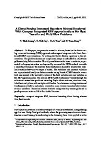
where κ¯ is the average fluid permeability for networks 1-4 without vesicle. The simulations were run on finite element mesh of size 26 × 31 (806 elements), sufficiently small to resolve the high curvature of the vesicle interface at large capillary numbers. Due to the presence of second order terms (e.g. the mean curvature) in the force generated by the vesicle-solvent surface tension, the explicit time evolutive simulations are subjected to a strict Courant-Friedrichs-Lewy (CFL) condition on the time step of the second order in mesh size dt ≈ O(∆h)2 , with ∆h the size of a single element. In this context, Fig. 7 shows the history of the non-dimensional speed of the vesicle vv /V as it travels through network 1 for capillary numbers Ca = 0.04 (Fig.7a) and Ca = 0.2 (Fig.7b). We observe that for a capillary number low enough (Ca = 0.04), the vesicle is too rigid to squeeze through the network (Fig. 7a). As a result, it remains trapped between two fibers while the surrounding fluid is diverted away from the obstructed pore. For higher capillary numbers (Ca = 0.2), the vesicle is slowed downed at the pore but is deformable enough to fully permeate through the same network (Fig 7b). These two example clearly indicate that deformation, in addition to size, dictate wether a vesicle can go through a porous medium. We further see that low deformability may result in the accumulation of trapped vesicles within the network and thus decrease the overall effective permability. This phenomenon is known as fouling [REF].
Figure 7: Vesicle speed as a function of non-dimensionalized time t ∗ for network 1, Ca = 0.04 (a) and Ca = 0.2 (b).
Let us now turn to the macroscopic effects of these observations. For this, we compute for each network and capillary numbers the macroscopic permeabilities
121
Particle-Based Moving Interface Method
Figure 8: Vesicle permeability as a function of the capillary number Ca =
Figure 9: Fluid permeability as a function of the capillary number Ca =
µU γ
µU γ
given in (44). For clarity, we particularly focus on understanding how the nondimensional vesicle and solvent permeabilities κv∗ and κs∗ change as functions of the capillary number Ca in Fig. 8 and Fig. 9 respectively. For all networks, we observe, as expected, that the vesicle permeability decreases with the capillary number, since less deformable vesicles have more difficulties squeezing through the tight pores. We also note that the vesicle permeability decreases to zero in the cases where the capillary number is low enough to cause the vesicle to be permanently trapped into the pores (fouling). On the other hand, the vesicle permeability is shown to approach that of the fluid without vesicle as the capillary number increases. Similarly, the solvent permeability κ ∗f is shown to decrease with the capillary
122
Copyright © 2014 Tech Science Press
CMES, vol.98, no.1, pp.101-127, 2014
number in Fig. 9. This is explained by the fact that more rigid vesicles hinder the fluid flow through the network, and that pores can be permanently obstructed by the most rigid vesicles. More importantly, even when pores are not obstructed, Fig. 9 shows that the presence of the vesicles can lessen the fluid permeability by as much as 20% for the network studied here. 5
Summary and future work
We have described a new numerical modeling approach that can be used to quantitatively examine the interplay between a rigid media’s structure, the surface energy of deformable, immiscible, suspended particles (vesicles), and an externally imposed continuum flow, on the particles’ conductance through that media. The novelty of the approach is two-fold: (a) the inclusion of locally-explicit continuum solutions for the pressure and velocity fields that eliminate the need for the computational cost of mesh refinement and (b) the derivation of a numerical homogenization scheme that permits to calculate the macroscopic permeabilities of a fibrous network for complex fluids. We have illustrated the usefulness of the approach by performing a study on an idealized two-dimensional problem containing deformable, "cylindrical-shaped" vesicles being transported in a simple fluid through a media containing rigid flakes (which project as "fibers" in our 2-d problem). The major macroscopic figures-of-merit were the permeability coefficients of the continuous fluid and the vesicles. For the range of parameters studied, our results have illustrated that vesicles are always retarded relative to the continuum flow, and that the relative selectivity for the continuum versus the vesicle is inversely proportional to the Capillary number (based on the vesicle’s surface energy relative to the continuum fluid). Overall, these results show the capability of the proposed approach to both accurately describe the micro-scale physics of a vesicle permeation, and their effects at the macroscale in terms of effective permeability estimations. A number of improvements is however necessary to increase the fidelity of the models. First, a thorough study of the physical interaction between fibers and vesicles must be carried out. For instance, the consideration of a repulsive force between the two entities in the proposed study ultimately facilitated the flow of vesicles away from fibers. In an alternate case, where fiber-vesicle adhesion occurs, one may predict very different behaviors [De Gennes, Brochard-Wyart, and Quere (2004)]. Our two-dimensional (2D) assumptions may also drastically affect the overall behavior of the system for several reasons. First, in 3D, one might expect a lower flow resistance from the fibers, but an increase in fiber-fiber connections, which might act as traps for vesicles. On the other hand, 3D vesicles possess more deformation potential to escape from these obstacles. From a modeling viewpoint, the proposed computational scheme is applicable in 3D although
Particle-Based Moving Interface Method
123
it is not straightforward. Asympotic flows around fibers and the deformation of 3D vesicles are indeed significantly more complex than in a 2D setting, involving numerous theoretical and numerical challenges. Such research endeavors are however necessary as a fundamental undertanding of the interactions between soft vesicles and porous media can help design new membranes for medical and energy applications [Gregoriadis and Florence (1993); Allen and Cullis (2013)], but also help understand fundamental problems in biology such as the interactions between cells and their surrounding fibrous matrix [Foucard and Vernerey (2012); Vernerey and Farsad (2011); Vernerey, Foucard, and Farsad (2011)]. Acknowledgement The authors gratefully acknowledge the National Science Foundation (NSF) Industry/University Cooperative Research Center for Membrane Science, Engineering and Technology (MAST) (formerly Membrane Applied Science and Technology) at the University of Colorado at Boulder (CU-B) for their support of this research via NSF Award IIP 1034720.
Appendix A: Using the spatial discretization scheme from section 3, the components of the matrix ke and vector fe take the following form:
Z
kvv = kevp = kevλ = kepv = keλ v = keλ p p = kepλ p =
Ωe
Z e ZΩ e ZΓ e ZΩ e ZΓ e ZΓ
Γe
µBT · B dΩ
(46a)
ˆ dΩ −BT · N
(46b)
¯ NT · NdΓ
(46c)
ˆ T · B dΩ N
(46d)
¯ T · NdΓ N
(46e)
ˆ ¯ T · NdΓ N
(46f)
ˆ T · NdΓ ¯ N
(46g)
124
Copyright © 2014 Tech Science Press
CMES, vol.98, no.1, pp.101-127, 2014
and fev feλ p
Z
= Ωe
Z
= Γe
T
N · ρf dΩ +
Z Γe
NT · (fI + fR/I ) dΓ.
(47)
¯ T n · (fI + fR/I ) dΓ. N
ˆ N ˆ and B take the following form: The shape function matrices N, N, � � ˜ 1 , ..., N ˜9 N = N1 , ..., N9 , N h i ˆ = Nˆ 1 , ..., Nˆ 4 , Nˇˆ 1 , ..., Nˇˆ 4 , N˜ˆ 1 , ..., N˜ˆ 4 N � � ¯ = N¯ 1 N¯ 2 N � � ˜9 B = B1 , ..., B9 , B˜ 1 , ..., B
(48)
(49a) (49b) (49c) (49d)
with Ni =
�
Ni 0 0 Ni
�
� � i � � i �� ˜ i = (F − F 1 ) N 0i , ..., (F − F 8 ) N 0i , N 0 N 0 N
(50a) � � ˇ ˜ i i i i 1 i 4 i Nˆ = (H − H )Nˆ , Nˆ = (G − G )Nˆ , ..., (G − G )Nˆ (50b) i N,1 0 0 N,2i Bi = (50c) Ni 0 ,2 0 N,1i (F − F 1 )N i ),1 0 (F − F 8 )N i ),1 0 0 (F − F 1 )N i ),2 0 (F − F 8 )N i ),2 , ..., . B˜ i = 8 i (F − F 1 )N i ),2 0 (F − F )N ),2 0 1 i 8 i 0 (F − F )N ),1 0 (F − F )N ),1 (50d) where F i and Gi are the asymptotic functions used to enriched the standard finite element space around the corner tips introduced earlier. References Alleborn, N.; Nandakumar, K.; Raszillier, H.; Durst, F. (1997): Further contributions on the two-dimensional flow in a sudden expansion. Journal of Fluid Mechanics, vol. 330, pp. 169–188.
125
Particle-Based Moving Interface Method
Allen, T. M.; Cullis, P. R. (2013): Liposomal drug delivery systems: from concept to clinical applications. Advanced drug delivery reviews, vol. 65, no. 1, pp. 36–48. Baker, R. (2004):
Membrane technology and applications. 2nd edition.
Baltus, R. E.; Badireddy, A. R.; Xu, W.; Chellam, S. (2009): Analysis of Configurational Effects on Hindered Convection of Nonspherical Bacteria and Viruses across Microfiltration Membranes. Industrial & Engineering Chemistry Research, vol. 48, no. 5, pp. 2404–2413. Cevc, G. (2004): Lipid vesicles and other colloids as drug carriers on the skin. Advanced drug delivery reviews, vol. 56, no. 5, pp. 675–711. Chen, Z.; Huan, G.; Ma, Y. (2006): Flows in Porous Media. SIAM.
Computational Methods for Multiphase
Cheryan, M. (2005): Membrane technology in the vegetable oil industry. Membrane Technology, vol. 2005, no. 2, pp. 5–7. De Gennes, P. G.; Brochard-Wyart, F.; Quere, D. (2004): Wetting Phenomena. Springer.
Capillarity and
Dechadilok, P.; Deen, W. M. (2006): Hindrance Factors for Diffusion and Convection in Pores. Industrial & Engineering Chemistry Research, vol. 45, no. 21, pp. 6953–6959. Desai, T. A.; Hansford, D. J.; Nashat, A. H.; Rasi, G.; Tu, J.; Wang, Y.; Zhang, M.; Ferrari, M. (2000): Nanopore Technology for Biomedical Applications. pp. 11–40. Dillon, R.; Owen, M.; Painter, K. (2008): A single-cell-based model of multicellular growth using the immersed boundary method. Contemporary Mathematics, vol. 466, no. 1, pp. 1–15. Eggleton, C. D.; Popel, A. S. (1998): Large deformation of red blood cell ghosts in a simple shear flow. Physics of Fluids, vol. 10, no. 8, pp. 1834. Faibish, R.; Elimelech, M.; Cohen, Y. (1998): Effect of Interparticle Electrostatic Double Layer Interactions on Permeate Flux Decline in Crossflow Membrane Filtration of Colloidal Suspensions: An Experimental Investigation. Journal of colloid and interface science, vol. 204, no. 1, pp. 77–86. Foucard, L.; Vernerey, F. J. (2012): A thermodynamical model for stress-fiber organization in contractile cells. Applied Physics Letters, vol. 100, no. 1, pp. 13702–137024. Foucard, L. C.; Vernerey, F. J. (2014): An X-FEM based numerical-asymptotic expansion for simulating a Stokes flow near a sharp corner. IJNME (under review).
126
Copyright © 2014 Tech Science Press
CMES, vol.98, no.1, pp.101-127, 2014
Foucard, L. C.; Vernerey, F. J. (2014): Particle-based Moving Interface Method for the study of immersed soft vesicles. IJNME (under review), pp. 1–31. Gregoriadis, G.; Florence, A. (1993): Liposomes in drug delivery. Clinical, diagnostic and ophthalmic potential. Drugs, vol. 45, no. 1, pp. 15–28. Hawa, T.; Rusak, Z. (2002): Numerical-Asymptotic Expansion Matching for Computing a Viscous Flow Around a Sharp Expansion Corner. pp. 265–281. Hoek, E. M. V.; Kim, A. S.; Elimelech, M. (2002): Influence of Crossflow Membrane Filter Geometry and Shear Rate on Colloidal Fouling in Reverse Osmosis and Nanofiltration Separations. Environmental Engineering Science, vol. 19, no. 6, pp. 357–372. Jason, H.; Kumar, T. (2012): Advances in Computational Dynamics of Particles, Materials and Structures. John Wiley & Sons, Ltd. Leung, S.; Lowengrub, J.; Zhao, H. (2011): A Grid Based Particle Method for Solving Partial Differential Equations on Evolving Surfaces and Modeling High Order Geometrical Motion. Journal of Computational Physics, vol. 230, no. 7, pp. 2540–2561. Leung, S.; Zhao, H. (2009): A grid based particle method for moving interface problems. Journal of Computational Physics, vol. 228, no. 8, pp. 2993–3024. Li, Y.; Yun, A.; Kim, J. (2011): An immersed boundary method for simulating a single axisymmetric cell growth and division. Journal of mathematical biology, vol. 65, no. 4, pp. 653–675. Ma, L.; Klug, W. S. (2008): Viscous regularization and r-adaptive remeshing for finite element analysis of lipid membrane mechanics. Journal of Computational Physics, vol. 227, no. 11, pp. 5816–5835. Moës, N.; Dolbow, J.; Belytschko, T. (1999): A finite element method for crack growth without remeshing. International Journal for Numerical Methods in Engineering, vol. 46, no. 1, pp. 131–150. Moffatt, H. K. (1963): Viscous and resistive eddies near a sharp corner. vol. 18, pp. 1–18. Mullin, T.; Seddon, J. R. T.; Mantle, M. D.; Sederman, a. J. (2009): Bifurcation phenomena in the flow through a sudden expansion in a circular pipe. Physics of Fluids, vol. 21, no. 1, pp. 014110. Peskin, C. (1972): Flow patterns around heart valves: A numerical method. Journal of Computational Physics, vol. 10, no. 2, pp. 252–271. Rabczuk, T.; Gracie, R.; Hsong, J.; Belytschko, T. (2000): Immersed Particle Method for Fluid-Structure Interaction. pp. 1–6.
Particle-Based Moving Interface Method
127
Song, L. (1998): Flux decline in crossflow microfiltration and ultrafiltration: mechanisms and modeling of membrane fouling. Journal of Membrane Science, vol. 139, no. 2, pp. 183–200. Vernerey, F.; Liu, W. K.; Moran, B. (2007): Multi-scale micromorphic theory for hierarchical materials. Journal of the Mechanics and Physics of Solids, vol. 55, no. 12, pp. 2603–2651. Vernerey, F. J. (2011): A theoretical treatment on the mechanics of interfaces in deformable porous media. International Journal of Solids and Structures, vol. 48, no. 22-23, pp. 3129–3141. Vernerey, F. J. (2012): The Effective Permeability of Cracks and Interfaces in Porous Media. Transport in Porous Media, vol. 93, no. 3, pp. 815–829. Vernerey, F. J.; Farsad, M. (2011): A constrained mixture approach to mechanosensing and force generation in contractile cells. Journal of the mechanical behavior of biomedical materials, vol. 4, no. 8, pp. 1683–99. Vernerey, F. J.; Foucard, L.; Farsad, M. (2011): Bridging the Scales to Explore Cellular Adaptation and Remodeling. BioNanoScience, vol. 1, no. 3, pp. 110–115. Zhang, L.; Gerstenberger, A.; Wang, X. (2002): Immersed Finite Element Method. Computer Methods in Applied Mechanics and Engineering, , no. September 2003, pp. 1–25.