Particle Filter Based Sensor Selection in Binary Sensor Networks

389

Particle Filter Based Sensor Selection in Binary Sensor Networks Yvo Boers and Hans Driessen THALES Nederland B.V. Linda Schipper Xsens Technologies B.V. Abstract – This paper is concerned with the application of target tracking in a network of sensors that provide binary output. The binary sensor network tracking problem is formulated in a sequential Bayesian estimation framework and is readily solved by means of a particle filter. We will perform sensor selection by means of a newly proposed scheme. This proposed approach is especially suitable for problems that exhibit non-Gaussian and multi modal behavior in the a posteriori density. We will show that the newly proposed selection scheme can also be extended to the multi target case. In addition, we also formulate a fairly simple sequential approximation of the proposed scheme that dramatically reduces the size of the associated optimization problem.

such a relatively small wireless sensor node. This sensor node is equipped with a seismic sensor.

Keywords: sensor networks, particle filters, target tracking, sensor selection.

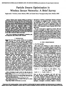
1 Introduction Systems, by means of which, distributed sensing, detection and tracking can be performed, become increasingly popular. This popularity is for a great part due to recent advances in wireless mobile communication technology and in Micro-Electro-Mechanical Systems. These technological advances have driven the feasibility for the use of lowcost and low-power sensor networks, see e.g [1]. Such a sensor network is composed of a (very large) number of sensor nodes, consisting of sensing, processing and communication components. Many types of sensors may be used, e.g. as visual, acoustic seismic, chemical or radar sensors, all depending on the specific application. In figure 1 we provide an example of

Figure 1: Example of a wireless sensor node: Thales Miniature Intrusion Sensor In this paper, we concentrate on a special type of sensor networks, namely networks in which sensors only provide binary output. These sensors or models of sensors arise in a lot of applications. Of course in practice most sensors from a physical standpoint are not binary, but when the signal corresponding to a measurement is thresholded only the excess or non-excess of this signal over a threshold is reported and the corresponding sensor model becomes binary. Possible reasons for using binary sensor models can be manifold. It can be e.g. from a standpoint of data reduction, or simply because it is the only information available to the user. We will model such a binary sensor network and show that inside the context of a generalized Bayesian filtering ap-

390 The new contributions of this paper are: • A new particle filter based scheduling mechanism for sensor selection, selecting recursively those sensors that cover the most probability mass of the predictive density. • A sequential approximative implementation of this algorithm, dramatically reducing the computational load of the selection algorithm.

Figure 2: Example of raw sensor data and binary data obtained by applying a threshold

2 System setup and problem formulation The system setup can be mathematically described by the following equations.

proach one can solve the filtering problem by employing a particle filter. Often in a distributed sensing application saving energy is key for the sensor nodes. This is the case because the nodes are typically battery operated and should work without requiring service for as long as possible. Therefore nodes should only sense and send their information if needed. In this paper, we will not deal with the communication part of the network, i.e. with the aspects of sending the messages or sensing reports through the network, but only with the sensing part. Furthermore, we will show that by employing a simple and efficient sensor selection mechanism we are able to use only a limited number of the sensors and still get a satisfactory performance. To the best of our knowledge, the idea of using a particle filter for a binary sensor network approach has been first proposed in [2]. A similar modelling approach has also been used in [3]. In fact in [2] also a sensor scheduling mechanism is employed with the aim of minimizing the number of sensor and thus the energy spent. However in [2] the scheduling approach is based on a covariance based technique and some heuristics, as articulated by the authors. Apart from the heuristic part, it is known and also shown in the proceeding of this paper, see section 2, that the nature of the a posteriori filtering distribution can be quite wild and multi modal. This makes a covariance measure not a very suitable selection mechanism. Therefore, in this paper we propose a selection method that exploits the full detailed extent of the a posteriori distribution by focussing on the maximum probability mass of the predictive density.

sk+1

∼

p (sk+1 |sk )

zk

∼

p (zk |sk ) ,

(1a) with

k∈N

(1b)

where

• sk is the state of the system at time k, • zk the measurement at time k. In the above discrete time system the state is defined as the two dimensional position and velocity and is thus four dimensional. The probability density function p(sk+1 |sk ) is completely determined by the system dynamics: sk+1

= F sk + Gwk

(2)

with wk being standard i.i.d. Gaussian noise 

1 0  0 1 F =  0 0 0 0

T 0 1 0

 0 T   0  1

(3)

and   G= 

1 1 2 2 ( 3 amax )T

0

1 3 amax T

0

0 1 1 2 2 ( 3 amax )T

0

1 3 amax T

   

(4)

391 where amax is the maximum acceleration and T the sample or update time of the system. Now for the measurement part of the system. For a single sensor j ∈ {1, . . . , M }, where M is the number of sensors, the measurement is binary, i.e. either 0 or 1 and the likelihood is, dropping the subscript for the time step: p(z j |s) = 1Rj (s)[z j (pjd + (1 − pjd )pjf a )+

see [4]. However, the optimal filtering can very well be implemented numerically by a particle filter, see [4]. In such a case a particle filter describes approximately the density of interest, p(sk | Zk ), where Zk denotes the measurement history, Zk = {z0 , . . . , zk }. The density is approximated by means of a (weighted) set of particles. {sik , wki }i=1,...,N

(5)

+(1 − z j )(1 − pjd )(1 − pjf a )]+ +(1 − 1Rj (s))[z j pjf a + (1 − z j )(1 − pjf a )] where 1Rj (s) is the indicator function, assuming either a value of 1 or 0, indicating whether the state of the object is inside the sensing range of sensor j or not. Furthermore, pjd and pjf a are the detection and false alarm probabilities of sensor j.

(6)

A graphical representation of such a filter ’in action’ in a sensor network application can be seen in figure 4. The particle cloud displayed in this figure also nicely displays the obvious non-Gaussian, in fact multi modal nature of the problem. This once more illustrates the need for a filter, e.g. a particle filter, that is able to cope with such phenomena. 80

70

The total likelihood p(z|s) is obtained as the product of the individual likelihoods.

50

y (m)

An example of a sensor network layout is provided in figure 3. Here the crosses indicate the sensor locations and the circles the sensing ranges.

60

40

30

7000

20

6000

10 5000

0

y (m)

4000

3000

0

10

20

30

40 x (m)

50

60

70

80

Figure 4: Particle description of p (sk |Zk )

2000

3 Sensor selection

1000

0 0

1000

2000

3000 x (m)

4000

5000

6000

7000

Figure 3: Example of a sensor network layout The filtering or tracking problem associated with the above system amounts to constructing the a posteriori density on the current state given all measurements up to the current time step. The filtering problem for the above system is not a standard one. This is due to the discontinuity of the likelihood function. The filter can therefore not be implemented by standard Kalman recursions, or even by an UKF,

As mentioned in the introduction, often there are only a limited number of sensors, whose information can be processed. Let us assume that for L out of a total of M sensors we are allowed to access and use the measurements. The problem now becomes one of choosing the L ’best’ sensors. Of course formally one would have to specify best in some sense, and from that hopefully a strategy can be deduced and implemented. We, however take a slightly different approach. We will propose a strategy and show that this strategy can be easily implemented using a particle filter. We propose a new and fairly simple strategy for sensor selection. We call this strategy the maximum volume strategy

392 or MAXVOL strategy. The basic idea is to select the combination of sensors that covers the largest probability volume of the predictive density. The set of L indices I ⊂ {1, .., M } uniquely identifies the selected sensors. VI is the volume of the state space that is covered by the sensors identified by I. Thus we arrive at the following problem formulation. Z arg max I

p (sk+1 |Zk ) dsk+1

(7)

VI

Let us define the following indicator function ½ 1, sk+1 ∈ VI 1VI (sk+1 ) = 0, sk+1 ∈ / VI the integral of equation (7) can now be rewritten as Z p (sk+1 |Zk ) dsk+1 =

(8) Figure 5: Comparing the number of possible sensor combinations for the optimal method and the sequential method (9)

VI

Z

This number is considerably (many orders of magnitudes) smaller than the number of evaluations for the optimal combination, see also figure 5.

1VI (sk+1 )p (sk+1 |Zk ) dsk+1 = = Ep(sk+1 |Zk ) [1VI (sk+1 )] ≈

We also note that in the case where the sensors have no overlap the sequential method will result in the optimal combination.

N 1 X ≈ 1V (si ) N i=1 I k+1

Inspecting the above (approximative) equation shows that the problem is solved by choosing that combination of L sensors by which the most particles are covered.

In the simulation examples we will use the sequential method.

To arrive at the optimal sensor combination for the MAXVOL criterion all possible sensor combinations have to be considered. If a sensor network consists of M sen¡ ¢ sors and L sensors are to be selected, there are M L sensor combinations to be considered. For a reasonable number of sensors in a network and a reasonable number of sensors to select, the number of combinations to be considered can easily become very large, see figure 5.

4 Simulation results

The optimal sensor combination can be approximated by selecting sensors sequentially instead of selecting the optimal sensor combination out of all possible sensor combinations. Sequential selection amounts to first picking the best sensor then discarding this one and picking the next best and so on until L sensors have been selected. The number of combinations that have to be evaluated in this case is L−1 X i=0

M −i

(10)

In this section we will provide simulation results on the MAXVOL approach. It will be shown that with a limited amount of sensors one can attain a performance, at least after some transient phase, equal to the situation in which all sensors are used. The sensors have a sensing range as indicated, a detection probability of pd = 0.90 and a false alarm probability of pf a = 0.05. One target is present in the network at all time steps and N = 3000 particles. Furthermore, the maximum target acceleration has been set to amax = 15m/s and the update time is T = 2s. In figure 6 the scenario at hand is depicted. In fact in this figure the actual trajectory of the target is visible, this is indicated by the black line, as well as the estimated trajectory or equivalently, the track, indicated by the red line. The figure also shows the sensor network layout graphically.

393 7000

6000

5000

y (m)

4000

3000

2000

1000

0 0

1000

2000

3000 x (m)

4000

5000

6000

7000

Figure 6: Sensor network layout, trajectory and filter result at final time step We have performed 100 Monte Carlo runs for one scenario and averaged the results over these 100 runs. The resulting position and velocity errors are displayed in figure 7 and figure 8 respectively.

Figure 8: Velocity error of the MAXVOL criterion: (·) with 10 sensors, (?) with 20 sensors, (∗) with 40 sensors, (◦) with 60 sensors and (¦) with all sensors used without a strategy

Looking at the results, we can also see, that except for the transient phase we do not need so many sensors. Actually it is better to, if possible of course, use more sensors in the initial phase and less after the transient phase. For the described scenario we have looked at the minimal number of sensors needed at each time step in order to arrive at a performance that is equal to the optimal performance, i.e. the performance obtained when all sensors are used. The result of this test is shown in figure 9. Note that the results shown here are also an MC average over 100 runs. From figure 9 we see that initially we need about 100 of the 144 sensors and that this number rapidly decreases to about a minimum number needed of about 7 sensors. This number is reached already quite fast, that is after some 5 time steps. These results indicate that there is quite a payoff if one is allowed to use more sensors in the initial phase.

Figure 7: Position error of the MAXVOL criterion: (·) with 10 sensors, (?) with 20 sensors, (∗) with 40 sensors, (◦) with 60 sensors and (¦) with all sensors used without a strategy From the simulation results in figure 7 and figure 8 we can see that the initial errors are larger when only a limited number of sensors is used. However, after this transient phase, the target is tracked with the same accuracy as in the case, where all sensors are used.

We do want to emphasize that we have considered regularly placed sensors, but that similar results can be obtained for a network of more randomly placed sensors.

5 Extension to the multi target case In this section we indicate, without going into all the details, how the proposed approach for sensor selection can be readily extended to the multi target case.

394 100

Also the state of the above system is a so called joint state, where the different state vectors corresponding to the different targets form one joint state vector, again see e.g. [5].

90

80

Now, the MAXVOL criterion, defined for a single target can be extended for the multi target case by choosing those sensors that cover the maximum multi target volume

70

M

60

50

40

arg max

30

I

20

10

0

X

0

5

10

15

20

25 time k

30

35

40

45

50

Figure 9: Minimum number of sensors needed at each time step to obtain optimal performance In order to do so, we will first explain how the sensor network and target model of section 2 is extended to cover the multi-target case. We assume a multi target dynamics according to the following system description:

mk+1 ∈M

Z p (sk+1 , mk+1 |Zk ) dsk+1

(13)

VI

We have also performed simulations in a multi target setting, in which the particle filter outputs the approximate posterior density on the kinematic as well as the modal state. Thus, p (sk |Zk , mk ) and p (mk |Zk ). In figure 10 we present a snap shot of a running filter with the MAXVOL selection mechanism. In this scenario, initially no targets were present in the scene, after a while the first target appears and after yet another while the second one appears. At the time step shown, both targets are present and tracked by a limited number of sensors selected according to the MAXVOL criterion. 7000

6000

P r{mk+1 = j|mk = i} zk with

∼ p (sk+1 |sk , mk ) (11a) = Pij

(11b)

∼ p (zk |sk , mk )

(11c)

k∈N

In the system defined by equations (11) an extra variable mk ∈ M has been introduced. This variable is a so called mode variable and is a discrete valued variable, that in our case defines the number of targets present. M defines the set of possible modes. For this case we could choose e.g.: M = {0, 1, . . . , M axN of T argets}

5000

4000 y (m)

sk+1

(12)

Thus, we have defined a multiple mode process or system, see e.g. [4]. The mode process is assumed to follow a Markov process with transition probabilities defined by Pij . In this application the mode corresponds to the number of targets present at time step k. Thus, the model reflected by equations (11) allows for birth and death of targets, see e.g. also [5].

3000

2000

1000

0 0

1000

2000

3000 x (m)

4000

5000

6000

7000

Figure 10: Snap shot at end of multi (2) target scenario Selected sensors in black

6 Conclusions In this paper we have presented a binary sensor network framework. We have provided a fairly simple and conceptually appealing sensor selection mechanism. We have also shown that this mechanism combines well with a particle filter approach for solving the sequential Bayesian state

395 estimation problem. We have also shown that this selection scheme yields satisfactorily tracking results while using only a fraction of the total number of sensors. Furthermore, we have extended the formulations to the general multi target case. A possible avenue of future work is to explore how the proposed sensor selection mechanism compares with other selection schemes proposed in the recent literature, both in terms of performance as well as in terms of computational load. However, it has already been indicated that our proposed method with some slight modification, i.e. using more sensors in the initial phase, leads to optimal performance, at least in the single target case. As well an interesting topic is to consider the approach presented here for more involved multi target scenarios. Scenarios with closely spaced targets are specifically challenging. In [6] some fundamental aspects of such scenarios in combination with a joint state particle filter approach are presented. Some interesting aspects of track extraction for such scenarios are treated in [7]. Furthermore, it would be very interesting and worthwhile to include the cost of communicating the sensor reports to a processing unit into the optimization.

7 Acknowledgement This work has been partially financially supported by the Netherlands Organization for Scientific Research (NWO) under the Casimir program, contract number 018.003.004. Under this grant the first author also holds a part-time position at the Stochastic Systems and Signals group of the Applied Mathematics Department at the University of Twente.

References [1] I.F. Akyildiz, W. Su, Y. Sankarasubramaniam, E. Cayirci, ” Wireless sensor networks: a survey,” Computer Networks, vol. 38, p. 393-422, 2002. [2] T. Stevens and D. Morrell, Minimization of Sensor Usage for Target Tracking in a Network of Irregularly Spaced Sensors, IEEE Workshop on Statistical Signal Processing, September 2003, pp. 549552. [3] P.M. Djuric, M. Vemula and M.F. Bugallo. Signal processing by particle filtering for binary sensor networks. In Proceedings of IEEE Digitital Signal Processing Workshop, 2004.

[4] S. Arulampalam, N. Gordon and R. Ristic, ” Beyond the Kalman Filter - Paricle Filters for Tracking Applications,” Boston - London: Artech House 2004. [5] Y. Boers and J.N. Driessen. A Particle Filter Multi Target Track Before Detect Application. IEE Proceedings - Radar, Sonar and Navigation, vol. 151, no. 6, 2004. [6] Y. Boers and J.N. Driessen. The Mixed Labeling Problem in Multi Target Particle Filters. In Proceedings of FUSION 2007, Quebec City, Canada, July 2007. [7] H.A.P. Blom, E.A. Bloem, Y. Boers and J.N. Driessen. Tracking closely spaced targets: Bayes outpeformed by an approximation ? In Proceedings of FUSION 2007 Cologne, Germany, July 2008.