Particle image velocimetry and computational fluid

Harminder Singh

Particle image velocimetry and computational fluid dynamics applied to study the effect of hydrodynamics forces on animal cells cultivated in Taylor vortex bioreactor

Universidade Federal do São Carlor – UFSCar Programa de Pós-Graduação em Engenharia Química – PPGEQ Laboratório de Technologia de Cultivo Celular – LATECC

Orientador: Prof. Dr. Claudio Alberto Torres Suazo

São Carlos - SP Março 2016

UNIVERSIDADE FEDERAL DE SÃO CARLOS LABORATÓRIO DE TECHNOLOGIA DE CULTIVO CELULAR DEPARTAMENTO DE ENGENHARIA QUÍMICA

HARMINDER SINGH

PARTICLE IMAGE VELOCIMETRY AND COMPUTATIONAL FLUID DYNAMICS APPLIED TO STUDY THE EFFECT OF HYDRODYNAMICS FORCES ON ANIMAL CELLS CULTIVATED IN TAYLOR VORTEX BIOREACTOR

Tese apresentado ao Programa de Pós-Graduação em Engenharia Química para obtenção do titulo de doutor em Engenharia Química. Orientação: Prof. Dr. Claudio Alberto Torres Suazo

SÃO CARLOS - SP 2016

Ficha catalográfica elaborada pelo DePT da Biblioteca Comunitária UFSCar Processamento Técnico com os dados fornecidos pelo(a) autor(a)

S617p

Singh, Harminder Particle image velocimetry and computational fluid dynamics applied to study the effect of hydrodynamics forces on animal cells cultivated in Taylor vortex bioreactor / Harminder Singh. -- São Carlos : UFSCar, 2016. 203 p. Tese (Doutorado) -- Universidade Federal de São Carlos, 2016. 1. DNS. 2. LES-WALE. 3. RANS. 4. Viscous energy dissipation rate. 5. Turbulence. I. Título.

Agradecimentos First and foremost, I would like to sincerely thank the Almighty, the One True Lord, for blessing the knowledge, will power, patience and numerous other skills required to become a researcher. There are three direct contributors who have enabled me to reach this stage of completing this thesis: my supervisor Prof. Dr. Claudio A. T. Suazo, "doutorado sanduìche"supervisor Prof. Dr. Alain Liné and financial supporter CNPq, Brasil. Without the conjunction of these three stepping stones, this study would not have been feasible. For the financial support, i would like to offer my gratitude to the Conselho Nacional de Desenvolvimento Cientifico e Tecnologico (CNPq), Brasil for the postgraduate (processo nº 140756/2012-4) and "Doutorado Sanduíche"(processo nº - 241739/2012-8) Scholarship programs. I am really grateful to Prof. Dr. Claudio A. T. Suazo for always having faith in my capabilities, giving me space and independence, and at the same time guiding me through whenever needed. His vast knowledge and experience in the field of bioreactors always opened various doors when things looked bleak. Apart from his able guidance, friendliness and carefulness, his support will always be appreciated. On the third front, i am indebted to Prof Dr. Alain Liné for accepting me as his "doutorado sanduìche"student, his support, care and participation in this work even now, long after the program ended in April 2014. Sharing of his wonderful ideas, vast knowledge and experience in the field of hydrodynamics kept me alive and ticking, and gave direction every time i got a bit lost. Major part of this thesis work has been conducted under his able guidance, and his critique only enhanced the quality of this work. I am thankful to Prof Dr. Roberto de Campos Giordano and Prof. Dr. José Antônio Silveira Gonçalves for their support, and sharing of their thoughts which helped in the improvement of this work. I am also grateful to all of the technicians, post-grads, and staff of the Chemical Engineering department in making this an enjoyable place to work. Finally, I would like to give my heartfelt thanks to all the family members, especially my spouse Tatiana Villela de Andrade Monteiro, and friends for their support from the beginning to the end of this project. They are the indirect contributors which held my hand and kept me up and floating in this vast ocean so that i could benefit something from the direct contributors.

“Mamma Man seu kaj hai,man saddey sidd hoi|| A soul’s primal aim of being born as a human is to tame the mind. Only if the mind can be tamed, that a soul’s objective can be achieved. Kabeer

Resumo O biorreator de Vórtices de Taylor (TVB) está se tornando uma nova descoberta, devido ao seu cisalhamento mais suave e fluxo homogêoneo em comparações com os biorretores de tanque agitados. Na literatura acadêmica há pouca informação sobre este biorreator quanto a taxa de dissipação de energia viscosa (VEDR), que é o parêmetro ideal para caracterizar a morte celular, e seus aspectos geométricos, que afetam o cultivo das células animais, resultando em baixa eficiência. A presente pesquisa, portanto, objetivou focar na estimativa da VEDR de fluxo médio e de energia cinética turbulenta (TKE) no TVB usando os métodos: experimental de 2D de velocimetria das partículas por imagem (PIV) e númerico de dinâmica de fluídos computacional (CFD) com diferentes modelos de turbulência, principalmente a simulação numérica direta (DNS). E focar nos aspectos geométricos do impacto da área de apuramento entre o cilindo interno e externo e na forma da base do cilindro externo na estrutura de fluxo do TVB. Os dois métodos experimental e númerico demonstraram que, em aproximadamente 80 % da área lateral entre os cilindros interno e externo onde as células vão passar a maior parte do tempo, a magnitude de velocidade é de cerca de 50 % da máxima e os valores de VEDR são 10 vezes menores do que nas paredes. Qualitativamente, o DNS mostrou boas comparações dos fluxos médios e dos parâmetros turbulentos em relação aos resultados apresentados pelo PIV para o TVB. No entanto, quantitativamente, apenas as previsões médias de velocidade estão em boa concordância com os dados do PIV, pois os parâmetros turbulentos foram sub-estimados. Entre os diferentes modelos de turbulência utilizados, o modelo simulação de grande escala (LES) - Wall Adapting Local EddyViscosity apresentou a melhor comparação com os dados do DNS para todos os parâmetros do fluxo. O modelo de estresse Reynolds e LES - Smagorinsky, por sua vez, apresentaram as piores comparações. Os modelos de duas equações de RANS, entretanto, apesar de estimarem bem os componentes de velocidade média em comparação com os dados do modelo DNS, não captaram bem as estruturas de fluxo dos componentes de turbulência. Quanto aos aspectos geométricos, as alterações nas características da área de apuramento entre o cilindo interno e externo e a estrutura curva da base do cilindro externo, que são de importância prática em tanque agitados, neste estudo, afetaram negativamente o fluxo no TVB devido ao seu baixo componente de velocidade axial. Por fim, a comparação entre o TVB e o Spinner Flask, considerado também um biorretor com baixo cissalhamento, demostrou que para Re/ReT semelhante, os valores máximo e médio do VEDR foram sempre inferiores, e devido à diferença muito menor entre o os valores máximo e médio, o TVB apresenta estruturas mais uniformes em comparação com o Spinner Flask. Palavras-chave: DNS. LES-WALE. RANS. dissipação de energia viscosa. turbulência.

Abstract Taylor-Vortex reactor (TVB) is fast becoming the next bioreactor to culture animal cells due to milder shear and homogeneous flow structures through-out the bioreactor in comparison to the traditional stirred vessels. However, there is little information in the literature for the TVB on the viscous energy dissipation rate (VEDR), which is considered the ideal parameter to characterize the cell death, and its geometrical aspects, which may affect the culture of animal cells resulting in poor efficiency. Consequently, this work focuses on: the estimation of the VEDR of mean flow and turbulent kinetic energy (TKE) using an experimental 2D particle image velocimetry (PIV) method and a computational fluid dynamics (CFD) method using different turbulence models, principally the direct numerical simulation (DNS) model; and, the impact of the off-bottom clearance area and the external cylinder’s bottom shape on the flow structures of TVB. Both numerical and experimental methods confirm that the bulk zone comprising of the 80 % of the gap-width, where the cell cultures will spend most of the time, has a near constant velocity magnitude of around 50 % of the tip velocity and VEDR values which are around 10 times lower than at the walls. Qualitatively, the DNS model predicted well the flow structure of both mean and turbulence parameters in comparison with the experimental PIV predictions. However, quantitatively only the mean velocity predictions are in good agreement with the PIV data with certain amount of under-estimation of the turbulence parameters. Among different turbulence models, the large eddy simulation (LES) - wall adapting local eddy-viscosity (WALE) model presented best comparison with the DNS model data for all the flow parameters; while, the Reynolds stress model and the LES-Smagorinsky models were the poorest. On the other hand, the Reynolds averaged Navier-Stokes (RANS) based two equation models estimated well the mean velocity components in comparison with the DNS model data, but could not capture well the flow structures of the turbulence components. The geometrical features of curved surface of outer bottom and off-bottom clearance area which are of practical importance in stirred vessels, impact adversely the flow structures in the TVB due to poor axial velocity component. In comparison with the spinner vessel, a stirred tank type bioeactor but with lower shear, for similar Re/ReT ratio, the maximum and mean VEDR were always found to be of lower magnitude values, and due to much less difference between the maximum and the mean values, the TVB presents more uniform structures in comparison to the spinner vessel.

Keywords: DNS. LES-WALE. RANS. viscous energy dissipation rate. turbulence.

Lista de ilustrações Figura 1 – Annual sales of recombinant proteins and monoclonal antibodies in the 2008-2013 period. Source: Ecker, Jones e Levine (2015). . . . . . . . . .

31

Figura 2 – PIV system consisting of the TVB, laser, camera, synchronization system and computer. . . . . . . . . . . . . . . . . . . . . . . . . . . . 45 Figura 3 – Convergence statistics of moment of order one (a) and two (b) on a horizontal plane located at ZL =0.725 and radially at Rb =0.082. . . . . 48 Figura 4 – Concentration of particles in a horizontal plane in the TVB at two different rotational rates: 114 (the one behind) and 30 (the one in front) rpm without grid (a) and with a 32 square grid (b). . . . . . . . . . . 50 Figura 5 – Impact of particle size on the estimations of mean tangential velocity (a) and squared fluctuating velocity (b) for the horizontal plane located at Zh = 0.725 ± 0.005. . . . . . . . . . . . . . . . . . . . . . . . . . . 52 Figura 6 – Impact of time-step on the estimations of mean tangential velocity (a) and squared fluctuating velocity (b) for the horizontal plane located at Zh = 0.725 ± 0.005 using particle size of 20 µm. . . . . . . . . . . . . 54 Figura 7 – Influence of the time-step and particle size on the VEDR of mean flow kinetic energy. . . . . . . . . . . . . . . . . . . . . . . . . . . . . . . . . 55 Figura 8 – Radial profile of mean tangential velocity at different overlap ratios and ICS values at ZL = 0.725 ± 0.005. . . . . . . . . . . . . . . . . . . . . 56 Figura 9 – Radial profile of squared fluctuating tangential velocity at different overlap ratios and ICS values at ZL = 0.725 ± 0.005. . . . . . . . . . . 58 Figura 10 – Radial profile of the viscous dissipation of mean flow kinetic energy at different overlap ratios and ICS values at ZL = 0.725 ± 0.005. . . . . 59 Figura 11 – Radial profile of the viscous dissipation of mean flow kinetic energy at different overlap ratios and ICS values at ZL = 0.725 ± 0.005. . . . . 60 Figura 12 – Radial profile of the viscous dissipation of turbulent kinetic energy at different overlap ratios and ICS values at ZL = 0.725 ± 0.005. . . . .

61

Figura 13 – Figure no 20 of Tokgoz et al. (2012) presenting dissipation rate estimations for changing interrogation window sizes (IW) for Res =14,000 with exact counter-rotation of cylinders. 75 % overalap ratio was used for all IWs. . . . . . . . . . . . . . . . . . . . . . . . . . . . . . . . . . 62 Figura 14 – Influence of the dimensionless spatial resolution of the maximum viscous dissipation of turbulent kinetic energy estimated at ZL = 0.725 ± 0.005 for different rotational speeds at different ICS and overlap ratios. . . . 62 Figura 15 – The tangential (a) and radial (b) velocity flow profiles at 114 rpm.

. . 64

Figura 16 – The tangential (a) and radial (b) velocity flow profiles at 90 rpm. . . . 65

Figura 17 – The tangential (a) and radial (b) velocity flow profiles at 70 rpm. . . . 66 Figura 18 – The tangential (a) and radial (b) velocity flow profiles at 50 rpm. . . . 67 Figura 19 – The tangential (a) and radial b) velocity flow profiles at 30rpm. . . . . 68 Figura 20 – The total viscosity at different rotational speeds in the center of vortex region. . . . . . . . . . . . . . . . . . . . . . . . . . . . . . . . . . . . .

71

Figura 21 – The evaluation of the constant C presented in the Equation 2.14. . . . 72 Figura 22 – The log-law profile of the velocity in the center of vortex region of the inner cylinder boundary layer. . . . . . . . . . . . . . . . . . . . . . . . 73 Figura 23 – The tangential (a) and radial (b) normal stress profiles at 114 rpm. . . 74 Figura 24 – The tangential (a) and radial (b) normal stress profiles at 90 rpm.

. . 75

Figura 25 – The tangential (a) and radial (b) normal stress profiles at 70 rpm.

. . 76


. . 77

Figura 27 – The tangential (a) and radial b) normal stress profiles at 30rpm. 0

0

Figura 28 – The Reynolds shear stress, ur uθ , profiles at 114rpm.

. . . . . . . . . . 80

0

. .

0

. . 82

Figura 29 – The Reynolds shear stress, u0r uθ , profiles at 90 (a) and 70 (b) rpm. 0

. . . 78

Figura 30 – The Reynolds shear stress, ur uθ , profiles at 50 (a) and 30 (b) rpm.

81

Figura 31 – The estimation of VEDR of mean flow kinetic energy and its 5 gradients at ZL = 0.725 ± 0.005. . . . . . . . . . . . . . . . . . . . . . . . . . . . 83 Figura 32 – The estimation of VEDR of turbulent kinetic energy and its 5 gradients at ZL = 0.725 ± 0.005. . . . . . . . . . . . . . . . . . . . . . . . . . . . 84 Figura 33 – Comparison of isotropy assumptions on radial profiles at ZL = 0.725 ± 0.005. . . . . . . . . . . . . . . . . . . . . . . . . . . . . . . . . . . . . 85 Figura 34 – Variation in the Kijkl ratios influenced by the dimensionless spatial resolution for the radial profiles located at ZL = 0.725 ± 0.005. . . . . . 86 Figura 35 – The VEDR of the mean flow, m , and turbulent, t , kinetic energy at 114 rpm. . . . . . . . . . . . . . . . . . . . . . . . . . . . . . . . . . . . 88 Figura 36 – The VEDR profiles of the mean flow, m , and turbulent, t , kinetic energy at 90 (a) and 70 (b) rpm. . . . . . . . . . . . . . . . . . . . . . 89 Figura 37 – The VEDR profiles of the mean flow, m , and turbulent, t , kinetic energy at 50 (a) and 30 (b) rpm. . . . . . . . . . . . . . . . . . . . . . 90 Figura 38 – The Kolmogorov scale for different rotational speeds at the center of vortex region. . . . . . . . . . . . . . . . . . . . . . . . . . . . . . . . . 93 Figura 39 – Geometry and mesh of the TVB used in the PIV experiments. . . . . . 103 Figura 40 – Comparison of different grid sizes for the DNS and LES models of dimensionless mean axial velocity (a), radial velocity (b), tangential velocity (c) and mean square of fluctuating tangential velocity (d) axially at Rb =0.067. The legend is same in all figures. . . . . . . . . . . . . . . 104 Figura 41 – Validation of the numerical DNS model with the PIV results of dimensionless mean tangential (a) and radial (b) velocity components. . . . . 107

Figura 42 – Validation of the numerical DNS model with the PIV results of the log-law profiles for the tangential component at the inner (a) and outer (b) boundary layers. The κ = 0.4 and B = 5.2 is used in the log profile. 108 Figura 43 – Validation of the numerical DNS model with the PIV results of dimensionless mean squared fluctuating tangential velocity component. . . . 109 Figura 44 – Validation of the numerical DNS model with the PIV results of the VEDR of mean flow (a) and turbulence (b) kinetic energy. . . . . . . . 110 Figura 45 – Identification of the Taylor’s vortexes through λ2 (a) and a pair of secondary Taylor’s vortexes (b) for the DNS model. . . . . . . . . . . . 116 Figura 46 – Identification of the Taylor’s vortexes through λ2 for the LES-WALE (a), and LES-Smagorinsky (b) models. . . . . . . . . . . . . . . . . . . 118 Figura 47 – Identification of the Taylor’s vortexes through λ2 for the k- (a) and RSM (b) models. . . . . . . . . . . . . . . . . . . . . . . . . . . . . . . 119 Figura 48 – Identification of the Taylor’s vortexes through λ2 for the SST (a), and SAS-SST (b) models. . . . . . . . . . . . . . . . . . . . . . . . . . . . . 120 Figura 49 – Radial profiles of the tangential velocity component near the outward region of a Taylor vortex. . . . . . . . . . . . . . . . . . . . . . . . . . 121 Figura 50 – Radial profiles of the tangential velocity component near the inward region of a Taylor vortex. . . . . . . . . . . . . . . . . . . . . . . . . . 121 Figura 51 – Radial profiles of the tangential velocity component near the center of vortex region of a Taylor vortex. . . . . . . . . . . . . . . . . . . . . . . 122 Figura 52 – Radial profiles of the radial velocity component near the outward region of a Taylor vortex. . . . . . . . . . . . . . . . . . . . . . . . . . . . . . 124 Figura 53 – Radial profiles of the radial velocity component near the inward region of a Taylor vortex. . . . . . . . . . . . . . . . . . . . . . . . . . . . . . 124 Figura 54 – Radial profiles of the radial velocity component near the center of vortex region of a Taylor vortex. . . . . . . . . . . . . . . . . . . . . . . . . . 125 Figura 55 – Radial profiles of the axial velocity component near the outward region of a Taylor vortex. . . . . . . . . . . . . . . . . . . . . . . . . . . . . . 126 Figura 56 – Radial profiles of the axial velocity component near the inward region of a Taylor vortex. . . . . . . . . . . . . . . . . . . . . . . . . . . . . . 126 Figura 57 – Radial profiles of the axial velocity component near the center of vortex region of a Taylor vortex. . . . . . . . . . . . . . . . . . . . . . . . . . 127 Figura 58 – Radial profiles of the log-law profiles of the axial mean of tangential velocity component for the inner (a) and outer (b) walls for the different turbulence models. . . . . . . . . . . . . . . . . . . . . . . . . . . . . . 128 Figura 59 – Radial profiles of the log-law profiles for the inner (a) and outer (b) walls near the outward, center of vortex and inward regions of a Taylor vortex for the DNS model only. . . . . . . . . . . . . . . . . . . . . . . 130

Figura 60 – Radial profiles of the tangential velocity component near the outward region of a Taylor vortex. . . . . . . . . . . . . . . . . . . . . . . . . . 131 Figura 61 – Radial profiles of the tangential velocity component near the inward region of a Taylor vortex. . . . . . . . . . . . . . . . . . . . . . . . . . 131 Figura 62 – Radial profiles of the tangential velocity component near the center of vortex region of a Taylor vortex. . . . . . . . . . . . . . . . . . . . . . . 132 Figura 63 – Radial profiles of the radial velocity component near the outward region of a Taylor vortex. . . . . . . . . . . . . . . . . . . . . . . . . . . . . . 132 Figura 64 – Radial profiles of the radial velocity component near the inward region of a Taylor vortex. . . . . . . . . . . . . . . . . . . . . . . . . . . . . . 133 Figura 65 – Radial profiles of the radial velocity component near the center of vortex region of a Taylor vortex. . . . . . . . . . . . . . . . . . . . . . . . . . 133 Figura 66 – Radial profiles of the axial velocity component near the outward region of a Taylor vortex. . . . . . . . . . . . . . . . . . . . . . . . . . . . . . 134 Figura 67 – Radial profiles of the axial velocity component near the inward region of a Taylor vortex. . . . . . . . . . . . . . . . . . . . . . . . . . . . . . 134 Figura 68 – Radial profiles of the axial velocity component near the center of vortex region of a Taylor vortex. . . . . . . . . . . . . . . . . . . . . . . . . . 135 Figura 69 – Radial profiles of the tangential velocity component near the outward region of a Taylor vortex. . . . . . . . . . . . . . . . . . . . . . . . . . 137 Figura 70 – Radial profiles of the tangential velocity component near the inward region of a Taylor vortex. . . . . . . . . . . . . . . . . . . . . . . . . . 138 Figura 71 – Radial profiles of the tangential velocity component near the center of vortex region of a Taylor vortex. . . . . . . . . . . . . . . . . . . . . . . 138 Figura 72 – Radial profiles of the radial velocity component near the outward region of a Taylor vortex. . . . . . . . . . . . . . . . . . . . . . . . . . . . . . 139 Figura 73 – Radial profiles of the radial velocity component near the inward region of a Taylor vortex. . . . . . . . . . . . . . . . . . . . . . . . . . . . . . 139 Figura 74 – Radial profiles of the radial velocity component near the center of vortex region of a Taylor vortex. . . . . . . . . . . . . . . . . . . . . . . . . . 140 Figura 75 – Radial profiles of the axial velocity component near the outward region of a Taylor vortex. . . . . . . . . . . . . . . . . . . . . . . . . . . . . . 140 Figura 76 – Radial profiles of the axial velocity component near the inward region of a Taylor vortex. . . . . . . . . . . . . . . . . . . . . . . . . . . . . . 141 Figura 77 – Radial profiles of the axial velocity component near the center of vortex region of a Taylor vortex. . . . . . . . . . . . . . . . . . . . . . . . . . 141 Figura 78 – Radial profiles of the turbulent kinetic energy near the outward region of a Taylor vortex. . . . . . . . . . . . . . . . . . . . . . . . . . . . . . 143

Figura 79 – Radial profiles of the turbulent kinetic energy near the inward region of a Taylor vortex. . . . . . . . . . . . . . . . . . . . . . . . . . . . . . . . 144 Figura 80 – Radial profiles of the turbulent kinetic energy near the center of vortex region of a Taylor vortex. . . . . . . . . . . . . . . . . . . . . . . . . . 144 Figura 81 – Comparison of the modeled turbulent kinetic energy with the one estimated from the velocity data in the center of vortex region of a Taylor vortex. . . . . . . . . . . . . . . . . . . . . . . . . . . . . . . . . 145 Figura 82 – Presentation of anisotropy through Lumley-Newmann and AG graphs axially near the walls, a) and b), and radially at the outward, center of vortex and inward regions of Taylor vortex, c) and d) respectively, for the DNS model. Note: in part a) and b) * represent the data near the inner and outer boundaries, while in c) and d) o, + and pentagram represent the outward, center of vortex and inward regions, respectively. 147 Figura 83 – The twelve gradients of the VEDR of mean flow (a) and turbulent (b) kinetic energy for the DNS model. . . . . . . . . . . . . . . . . . . . . 149 Figura 84 – The estimation of the VEDR of mean flow and turbulent kinetic energy of the DNS model in the outward, center of vortex and inward regions . 150 Figura 85 – The Kolmogorov estimations of the DNS model calculated through the VEDR of turbulent kinetic energy for the respective model and the mesh size. . . . . . . . . . . . . . . . . . . . . . . . . . . . . . . . . . . 152 Figura 86 – The estimation of the VEDR of TKE for the different turbulence model for axial mean of all the radial profiles. . . . . . . . . . . . . . . . . . . 153 Figura 87 – Three different shapes of the outer bottom cylinder at 15 mm offbottom clearance and 1.968 × 106 , 2.24 × 106 and 2.22 × 106 node meshes, respectively, for each geometry. Green and purple markers signify interface area and periodic boundaries respectively. Please note that not all interface areas and periodic boundaries are shown here. . . 160 Figura 88 – Radial flow profiles of the mean velocity for the mesh and time-step independence study in the TVB with 5 mm off-bottom clearance and flat bottom at ZL =0.57. . . . . . . . . . . . . . . . . . . . . . . . . . . 163 Figura 89 – Mean velocity comparisons between the sliding mesh and MRF techniques in the TVB with 5 mm off-bottom clearance and flat bottom at ZL =0.57. . . . . . . . . . . . . . . . . . . . . . . . . . . . . . . . . . . 164 Figura 90 – Comparison of numerical tangential velocity results with the PIV results of (COUFORT; BOUYER; LINE, 2005). . . . . . . . . . . . . . . . . . 166 Figura 91 – Velocity and its three components in an axial profile located at Rb =0.009.167 Figura 92 – Vector profile of the secondary vortex. . . . . . . . . . . . . . . . . . . 167 Figura 93 – Dimensionless mean velocity at various radial (a) and axial positions (b).168 Figura 94 – Mean velocity vectors for different shapes and off-bottom clearance areas.170

Figura 95 – Dimensionless mean velocity at different radial (a) and axial (b) positions for different geometry types. . . . . . . . . . . . . . . . . . . . . . . . . 171 Figura 96 – VEDR values for different hydrodynamic conditions in bioreactors and regions of lethal and sub-lethal impacts on cell lines. Adapted from Godoy-Silva et al. (2009). . . . . . . . . . . . . . . . . . . . . . . . . . 172

Lista de tabelas Tabela 1 – Various parameters used to correlate to cell death in a Stirred tank. . Tabela 2 – Dimensions and geometrical characteristics of the TVB used in the PIV system. . . . . . . . . . . . . . . . . . . . . . . . . . . . . . . . . . . . Tabela 3 – Analytical estimations for the TVB used in the PIV system. . . . . . Tabela 4 – Different ICS and overlap windows tested at ZL = 0.725 ± 0.005. . . . Tabela 5 – Dimensionless Spatial resolution,δ/hηi, for different rotational velocities, ICS values and overlap ratios located at ZL = 0.725 ± 0.005. . . . . . . Tabela 6 – Mesh configurations used to model the TVB. . . . . . . . . . . . . . . Tabela 7 – Torque and Power estimations in TVB through numerical and analytical methods. . . . . . . . . . . . . . . . . . . . . . . . . . . . . . . . . . . Tabela 8 – Dimensions and geometrical characteristics of the TVB used for studying the different geometrical structures. . . . . . . . . . . . . . . . . . . . Tabela 9 – Grid independence study with the flat-bottom TVB at 5 mm off-bottom clearance. . . . . . . . . . . . . . . . . . . . . . . . . . . . . . . . . . . Tabela 10 – Mean percentage difference of the mean velocity between different meshes. . . . . . . . . . . . . . . . . . . . . . . . . . . . . . . . . . . . Tabela 11 – Analytical and numerical estimations of the Taylor reactor at 200 rpm. Tabela 12 – Summary of VEDR and Kolmogorov micro-scales for different geometrical conditions. . . . . . . . . . . . . . . . . . . . . . . . . . . . . . .

34 44 46 47 60 103 154 159 162 163 173 173

Lista de abreviaturas e siglas CHO

Chinese Hamster Ovary

CFD

Computational Fluid Dynamics

DNS

Direct Numerical Simulation

ICS

Interogation Cell Size

LES

Large Eddy Simulation

LDA

Laser Doppler Anemometry

MFKE

Mean Flow Kinetic Energy

MRF

Multiple Reference Frame

OBC

Off Bottom Clearance

PIV

Particle Image Velocimetry

RANS

Reynolds Averaged Navier Stokes

RMS

Root Mean Square

RSM

Reynolds Stress Model

SAS

Scale Adaptive Simulation

SGS

Sub Grid Scale

SST

Shear Stress Transport

TKE

Turbulence Kinetic Energy

TVB

Taylor Vortex Bioreactor

VEDR

Viscous Energy Dissipation Rate

WALE

Wall Adapting Local Eddy

Lista de símbolos b

Gap width, ro - ri , m

bij

Reynolds stress anisotropy tensor, m2 s−2

d+

Radial coordinate at the inner wall, ruτ i /ν, (-)

C

Constant of SAS-SST turbulence model, 2, (-)

C1

Constant of k- model, 1.44 (-)

C2


C1RSM

Constant of LRR-IP RSM model, 1.45 (-)

C2RSM


C1RSM


C2RSM


Cµ


CS

LES-Smagorinsky constant, 0.2 (-)

CS−RAN S

Constant of LLR-RSM turbulence model, 0.22 (-)

CW

LES-WALE constant, 0.325 (-)

d+e

Radial coordinate at outer wall, re (= rmax − r)uτ e /ν, (-)

F1

Blending function for the SST turbulence model, (-)

F2

Blending function for the SST turbulence model, (-)

Gk

Generation of TKE for k- model, νt S 2 , m2 s−3

k

Turbulence kinetic energy, m2 s−2

L

Lenght of the outer cylinder, m

Lvk

von Karmen length scale, (-)

obc

Off-bottom clearance, m

p

Pressure, Pa

p’

Modified pressure for RANS based two equation models, Pa

p”

Modified pressure for RANS based RSM models, Pa

P

Power, P = τ ω=

RRR

ρdv, Watts

v

r

radial direction, m

ri

Inner cylinder radius, m

ro

Outer cylinder radius, m

Rb

Dimensionless radial coordinate,

r−ri , b

(-)

Re

Reynolds number,

Sij

Strain rate, s−1

Ta

Taylor number,

ri ω(ro −ri ) , ν

1/2

ri

(-)

ω(ro −ri )3/2 , ν

(-)

0

Fluctuating radial velocity component, ms−1

0

Fluctuating tangential velocity component, ms−1

uz

0

Fluctuating axial velocity component, ms−1

uτ i

Friction velocity at inner cylinder, ms−1

uτ e

Friction velocity at outer cylinder, ms−1

Uθ

Tangential component of the velocity, ms−1

Ur

Radial component of the velocity, ms−1

Utip

Tip velocity, rω, ms−1

Uz

Axial component of the velocity, ms−1

v

Volume of the reactor, m3

z

Axial direction, m

ZL

Dimensionless axial coordinate,

Viscous energy dissipation rate, m2 s−3

ur

uθ

z , L

(-)

hi

Mean viscous energy dissipation rate, m2 s−3

innerwall

Mean viscous energy dissipation rate at inner wall, u4τ /ν, m2 s−3

ηrr

Radius ratio,

η

Kolmogorov’s micro-scale, µm

δij

kronecker delta, (-)

∆

local gird scale, m

κ

von Kárman constant, (-)

Λ

Taylors’s micro-scale, mm

λ1 , λ2 andλ3

ri , ro

(-)

Three eigenvalues of the vector S 2 + Ω2 , s−2

ν

Kinematic viscosity, m2 s−1

νef f

Modified kinematic viscosity of RANS based models, ν + νt , m2 s−1

νsgs

Subgrid scale eddy viscosity, m2 s−1

νt

Turbulent viscosity of RANS based models, m2 s−1

η2

Constant of SAS-SST turbulence model, 3.51 (-)

Γ

Aspect ratio,

ρ

Density, kgm−3

L , b

(-)

σk


σkSST

Constant of SST turbulence model, 1/(F1 /σk,1 + (1 − F1 )σk,2 ), (-)

σk,1

Constant of SST turbulence model, 1.176 (-)

σk,2


σ


σ RSM


σωSST

Constant of SST turbulence model, 1/(F1 /σω,1 + (1 − F1 )σω,2 ), (-)

σω,1


σω,2 )


σΦ

Constant of SAS-SST turbulence model, 2/3 (-)

βi,1


βi,2


∗ β∞


τ

Torque, Nm

τw

Wall shear stress, N m−2

θ

Tangential direction, m

ω

Angular velocity, rads−1

ωtef

turbulence eddy frequency of k-ω models, s−1

Ωij

Rotation rate, s−1

Sumário 1

INTRODUCTION . . . . . . . . . . . . . . . . . . . . . . . . . . . . 31

1.1

Bioreactors and Hydrodynamics . . . . . . . . . . . . . . . . . . . . . 31

1.2

Understanding Hydrodynamics . . . . . . . . . . . . . . . . . . . . . . 36

1.2.1

Experimental method . . . . . . . . . . . . . . . . . . . . . . . . . . . . . 37

1.2.2

Numerical method-CFD . . . . . . . . . . . . . . . . . . . . . . . . . . . 38

1.3

Overall project . . . . . . . . . . . . . . . . . . . . . . . . . . . . . . . 41

1.3.1

Main aim of this thesis . . . . . . . . . . . . . . . . . . . . . . . . . . . . 42

2

EXPERIMENTAL METHOD - PIV . . . . . . . . . . . . . . . . . . 43

2.1

Description of case set-up . . . . . . . . . . . . . . . . . . . . . . . . . 43

2.2

PIV set-up . . . . . . . . . . . . . . . . . . . . . . . . . . . . . . . . . . 44

2.3

Estimation of VEDR . . . . . . . . . . . . . . . . . . . . . . . . . . . . 47

2.4

Basic Aspects of PIV . . . . . . . . . . . . . . . . . . . . . . . . . . . 49

2.4.1

Concentration of particles . . . . . . . . . . . . . . . . . . . . . . . . . . 49

2.4.2

Size of particles . . . . . . . . . . . . . . . . . . . . . . . . . . . . . . . . 51

2.4.3

Time-step between frames . . . . . . . . . . . . . . . . . . . . . . . . . . 53

2.4.4

Choosing overlap & ICS . . . . . . . . . . . . . . . . . . . . . . . . . . . 55

2.5

Results and discussion . . . . . . . . . . . . . . . . . . . . . . . . . . . 63

2.5.1

Mean velocity flow field . . . . . . . . . . . . . . . . . . . . . . . . . . . . 63

2.5.2

Logarithmic velocity profiles . . . . . . . . . . . . . . . . . . . . . . . . . 69

2.5.3

Reynolds stresses . . . . . . . . . . . . . . . . . . . . . . . . . . . . . . . 72

2.5.3.1

Normal stress

2.5.3.2

Shear Stress

2.5.4

Viscous energy dissipation rate . . . . . . . . . . . . . . . . . . . . . . . . 80

2.5.4.1

Composition of the VEDR

2.5.4.2

EDR structure

2.5.5

Kolmogorov scale . . . . . . . . . . . . . . . . . . . . . . . . . . . . . . . 92

2.6

Conclusions . . . . . . . . . . . . . . . . . . . . . . . . . . . . . . . . . 93

3

NUMERICAL METHOD AND ITS VALIDATION . . . . . . . . . . 97

3.1

Turbulence modelling . . . . . . . . . . . . . . . . . . . . . . . . . . . 97

3.2

Numerical methodology . . . . . . . . . . . . . . . . . . . . . . . . . . 102

3.2.1

Geometry and Meshing aspects . . . . . . . . . . . . . . . . . . . . . . . . 102

3.2.2

Pre-processing aspects . . . . . . . . . . . . . . . . . . . . . . . . . . . . 105

3.2.3

Solver & Post-processing aspects . . . . . . . . . . . . . . . . . . . . . . . 105

3.2.4

Estimation of VEDR . . . . . . . . . . . . . . . . . . . . . . . . . . . . . 105

. . . . . . . . . . . . . . . . . . . . . . . . . . . . . . . . . .

72

. . . . . . . . . . . . . . . . . . . . . . . . . . . . . . . . . . .

79

. . . . . . . . . . . . . . . . . . . . . . . . . . . .

80

. . . . . . . . . . . . . . . . . . . . . . . . . . . . . . . . . .

87

3.3

Validation of the computational model . . . . . . . . . . . . . . . . . 106

3.4

Conclusions . . . . . . . . . . . . . . . . . . . . . . . . . . . . . . . . . 113

4

TURBULENCE MODELS . . . . . . . . . . . . . . . . . . . . . . . . 115

4.1

Vortex identification . . . . . . . . . . . . . . . . . . . . . . . . . . . . 115

4.2

Mean velocity flow field . . . . . . . . . . . . . . . . . . . . . . . . . . 117

4.2.1

Tangential velocity . . . . . . . . . . . . . . . . . . . . . . . . . . . . . . 117

4.2.2

Radial velocity . . . . . . . . . . . . . . . . . . . . . . . . . . . . . . . . 123

4.2.3

Axial velocity . . . . . . . . . . . . . . . . . . . . . . . . . . . . . . . . . 123

4.2.4

Log law profiles of tangential velocity . . . . . . . . . . . . . . . . . . . . 125

4.3

Normal stresses . . . . . . . . . . . . . . . . . . . . . . . . . . . . . . . 129

4.4

Reynolds shear stresses . . . . . . . . . . . . . . . . . . . . . . . . . . 137

4.5

Turbulent kinetic energy . . . . . . . . . . . . . . . . . . . . . . . . . . 143

4.6

Anisotropy . . . . . . . . . . . . . . . . . . . . . . . . . . . . . . . . . . 145

4.7

Viscous energy dissipation rate . . . . . . . . . . . . . . . . . . . . . . 147

4.7.1

Composition of VEDR . . . . . . . . . . . . . . . . . . . . . . . . . . . . 147

4.7.2

Structure of VEDR . . . . . . . . . . . . . . . . . . . . . . . . . . . . . . 149

4.7.3

Power Estimation . . . . . . . . . . . . . . . . . . . . . . . . . . . . . . . 153

4.8

Conclusions . . . . . . . . . . . . . . . . . . . . . . . . . . . . . . . . . 154

5

AN APPLICATION OF CFD . . . . . . . . . . . . . . . . . . . . . . 157

5.1

Problem description . . . . . . . . . . . . . . . . . . . . . . . . . . . . 157

5.2

Computational model . . . . . . . . . . . . . . . . . . . . . . . . . . . 159

5.2.1

Description of case set-up . . . . . . . . . . . . . . . . . . . . . . . . . . 159

5.2.2

Turbulence modeling . . . . . . . . . . . . . . . . . . . . . . . . . . . . . 161

5.2.3

Computational mesh and time-step

5.2.4

Sliding mesh or MRF technique . . . . . . . . . . . . . . . . . . . . . . . 162

5.2.5

Computational aspects . . . . . . . . . . . . . . . . . . . . . . . . . . . . 165

5.3

Validation of the computational model . . . . . . . . . . . . . . . . . 165

5.4

Results and discussion . . . . . . . . . . . . . . . . . . . . . . . . . . . 166

5.4.1

Mean velocity flow field . . . . . . . . . . . . . . . . . . . . . . . . . . . . 166

5.4.2

Outer cylinder’s bottom shapes

5.4.3

Off-bottom clearance . . . . . . . . . . . . . . . . . . . . . . . . . . . . . 170

5.4.4

Viscous energy dissipation rate(VEDR)

5.5

Conclusions . . . . . . . . . . . . . . . . . . . . . . . . . . . . . . . . . 176

6

CONCLUSIONS . . . . . . . . . . . . . . . . . . . . . . . . . . . . . 179

. . . . . . . . . . . . . . . . . . . . . 161

. . . . . . . . . . . . . . . . . . . . . . . 169 . . . . . . . . . . . . . . . . . . . 172

Referências . . . . . . . . . . . . . . . . . . . . . . . . . . . . . . . . 183

APÊNDICE A – MATLAB FILE . . . . . . . . . . . . . . . . . . . . 193

Índice . . . . . . . . . . . . . . . . . . . . . . . . . . . . . . . . . . . 203

31

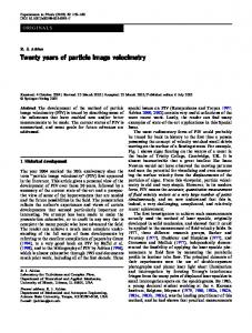
1 Introduction 1.1 Bioreactors and Hydrodynamics The cultivation of animal cells (including human), a sub-area of biotechnology, in in vitro is a process of over 100 years old, but the emerging need of vaccines in the 1950s imparted some momentum to this process leading to the development of various vaccines such as measles (1963), rabies (1964), mumps (1967) and rubella (1969) (KRETZMER, 2002). In the mid-1970s, a second set of products hit the market - monoclonal antibodies by forming hybridomas from the fusion of cells, and genetic engineering (KRETZMER, 2002).f Nowadays, the animal cell product list has increased to a huge number, namely, human and veterinary vaccines, diagnostics monoclonal antibodies and therapeutics, such as tPA, erythropoietin and interferons, with many animal cell products being highly costly in the order of US $ 104 to $ 109 per kilogram (KRETZMER, 2002; ECKER; JONES; LEVINE, 2015). The ever-increasing sales forecasts of the recombinant proteins and monoclonal antibodies till 2013 presented by Ecker, Jones e Levine (2015) can be seen in Figure 1, of which currently ≈ 54 % are being produced by animal cells (ECKER; JONES; LEVINE, 2015).

Figura 1 – Annual sales of recombinant proteins and monoclonal antibodies in the 20082013 period. Source: Ecker, Jones e Levine (2015). To achieve maximum yields, it becomes important to provide the cells with an in vitro environment as similar as possible to the natural cell environment, leading to studies regarding the composition of culture media, process controls (pH, temperature, dissolved oxygen), and especially the bioreactors. Major improvements, mainly, in the

32

Capítulo 1. Introduction

culture media composition and process control, have resulted in over 100-fold yield increase in the cultivation of mammalian cells in the bioreactors for similar processes that were used in the mid-1980s (WURM, 2004). Nonetheless, there are still possibilities of further improvements in the yield through the optimization of various processes in the cultivation of animal cells (KRETZMER, 2002; WURM, 2004; JAIN; KUMAR, 2008; COSTA et al., 2010). One of the most crucial factors that play a significant role in the design of a bioreactor using animal cells is that they do not possess a cell wall, unlike bacteria, fungi and plant cells. Lack of cell wall makes the animal cells extremely sensitive to external environment such as pH, temperature, nutrients or culture media, regulatory molecules, oxygenation through bubbling and hydrodynamic forces resulting from aeration through bubbling and agitation in a bioreactor. These unique characteristics of animal cells makes it imperative to develop bioreactors designed with agitation and oxygenation systems that generate hydrodynamic forces milder than those found in bioreactors cultivating microbes (NIENOW, 2006). Presently, the two most commonly employed bioreactors in large scale are the stirred or agitated tank and airlift reactor (CHU; ROBINSON, 2001; KRETZMER, 2002; JAIN; KUMAR, 2008; NIENOW, 2006). From the 30 L in the 1960s to 8,000 L in 1980s to 20,000 L in the mid-2000s has been the increase in the capacity of a traditional agitated bioreactor to produce vaccines, monoclonal antibodies and therapeutics (NIENOW, 2006; KRETZMER, 2002). On the other hand, the airlift bioreactor has been scaled up-to 2,000 L to produce monoclonal antibodies with reports of a 10,000 L airlift bioreactor which successfully cultured hybridoma cells to produce monoclonal antibodies (JAIN; KUMAR, 2008). Although, both bioreactor types have the versatility of cultivating both suspension and anchorage-dependent cells, the stirred tank has been the preferred choice of the industrialists due to easy scale-up, homogeneous environment and vast industrial experience of working with this reactor type (CHU; ROBINSON, 2001; NIENOW, 2006). However, certain cell lines demand a surface for adherent culture systems which lead to the development of high density cell culture systems, such as hollow fiber, packed bed and fluidized-bed bioreactors (JAIN; KUMAR, 2008). Although, these compact bioreactors have the advantage of high volumetric productivity, they suffer from concentration gradients due to non-homogeneity and difficulty in monitoring and scale-up (OZTURK, 1996). Disposable bioreactor is another genre that has entered the market in the start of the twenty-first century largely to reduce hydrodynamic stress and process cost, and have easier process control, for example, wave bioreactor (SINGH, 1999). Although, wave bioreactors have been scaled up-to 1,000 L capacity (JAIN; KUMAR, 2008), industrial-scale capacities are still under question. Another disposable bioreactor is being developed by the Jain e Kumar (2008) group, named cryogel bioreactor, with a capacity of up-to 1L and functioning similar

1.1. Bioreactors and Hydrodynamics

33

to that of hollow fiber bioreactor. In addition, in recent years, another reactor type, named Taylor-Vortex Bioreactor (TVB) has emerged as a choice for culturing cells (O’CONNOR et al., 2002; HAUT et al., 2003; CURRAN; BLACK, 2004; CURRAN; BLACK, 2005; GONG et al., 2006; TANZEGLOCK, 2008; SANTIAGO; GIORDANO; SUAZO, 2011; ZHU et al., 2010). These researchers successfully cultured various animal and insect cell lines, namely Chinese Hamster Ovaries (CHO), Human Embryonic Kidney, rat bone marrow stroma, and Sf-9 Spodoptera frugiperda, in suspension in a TVB. The oxygen is easily provided through gaspermeable membranes in these reactor types thus reducing the hydrodynamic stress due to aeration by bubbling (CURRAN; BLACK, 2005; SANTIAGO; GIORDANO; SUAZO, 2011). Another advantage of the TVB is the possibility of scale-up to an industrial level bioreactor, thus making it a serious contender for culturing animal cells (CHAUDHURI; AL-RUBEAI, 2005). The design, scale-up and operation of bioreactors for animal cell culture require a comprehensive understanding of the mechanisms of cell damage and death caused by the fluid-mechanical forces associated with the equipment type (BRIONES; CHALMERS, 1994). Therefore, the parameters characterizing the effect of hydrodynamic forces causing cellular destruction are of crucial importance in the validation of bioprocess development studies conducted primarily in the mini-bioreactors and later transferred to the larger-scale bioreactors. Numerous parameters have been used to characterize cell death or damage in the various studies, as shown in Table 1, and a consensus has not been reached. Moreover, there is little information available on how to use flow parameters that correlate well with cell damage in one particular system to predict cell damage in a different system. Briones e Chalmers (1994) stated that cell damage should ideally be predicted by knowing the actual stresses that the cell experiences, determined from intrinsic cell mechanical properties and the resulting cell deformation. Should the cell deformation exceed a critical value, the disruption of the cell structure would be expected. They suggested that the parameter chosen to correlate with cell damage should be 1) general in nature and not be dependent on the particular geometry and 2) be local, that is, not be averaged throughout the flow domain. Briones e Chalmers (1994) rejected the Kolmogorov eddy scale as a basis for predicting cell damage, because essentially cell size becomes the only correlation parameter when this parameter is used, and therefore cell mechanical properties are neglected. Kunas e Papoutsakis (1990) suggested that, although Kolmogorov eddy length can be used as a predictor of cell damage, it does not provide any details of how cells are damaged by their interaction with these eddies or even prove that there is a direct cell-eddy interaction. Echoing this sentiment, Joshi, Elias e Patole (1996) stated that it is very difficult to predict the relationship between the eddy size and its role in cell damage.

34


Tabela 1 – Various parameters used to correlate to cell death in a Stirred tank. Cells used

Range of hydrodynamic Parameters Insect Cells, 210- 510 rpm τ = 3 SF-21 N/m2 Cell death rate proportional to volumetric gas flow rate Hybridoma, 60-900 rpm, Cell deCRl-8018 ath correlates to Kolmogorov eddy size similar to or smaller than the cell

Important Observati- Reference ons “Viability of cells de- Tramper et al. creased at shear stres- (1986) ses of 1 N/m2 ”

“In absence of gas sparging, cells are damaged only at speed above 700 rpm. No damage at speeds less than 600 rpm” Hybridoma, 100-440 rpm, Impeller “ Death rate constant, HDP-1 tip speed 19-73.3 cm/s kd , increased sharply at impeller tip speeds above 40 cm/s” SF-9 and < 0.7 impeller tip “Damaging threshold Hybridoma, speed, < 350 W/m3 values of impeller serum con- Power Inputs tip speed or specific taining, gas Power inputs for some free animal cells”

Kunas e Papoutsakis (1990)

Abu-Reesh e Kargi (1989)

Chisti (2001)

In the last 15 years, the group of Prof. Jeffrey Chalmers from the Ohio state university in USA have presented various meticulous studies of probably the ideal parameter to characterize the potential of hydrodynamic stresses to damage cells (GREGORIADES et al., 2000; MA; KOELLING; CHALMERS, 2002; MOLLET et al., 2004; MOLLET et al., 2007; MOLLET et al., 2008; GODOY-SILVA et al., 2009; GODOY-SILVA; MOLLET; CHALMERS, 2009). There have been various studies estimating the lethal effects of Viscous energy dissipation rate (VEDR) on cell cultures using various types of devices, such as microfluidic channel, contractional flow device and capillary flow device (THOMAS; AL-RUBEAI; ZHANG, 1994; ALOI; CHERRY, 1996; GREGORIADES et al., 2000; MA; KOELLING; CHALMERS, 2002; MOLLET et al., 2007). According to Ma, Koelling e Chalmers (2002), lethal VEDR are at least 1000 times greater than those used in stirred tank bioreactors operated successfully in sizes ranging from 10 L and 22,000 L capacity. The cell cultures of Ma, Koelling e Chalmers (2002) were tested in a transient flow contractional device with residence times similar to a stirred tank having a rotational speed of 500 rpm. However, these cells were exposed to high levels of VEDR only once, as in the research work of Thomas, Al-Rubeai e Zhang (1994), Aloi e Cherry (1996), Gregoriades et al. (2000), Mollet et al. (2007). The cells in a stirred tank are exposed multiple times to high levels of turbulent VEDR in the vicinity of the impeller due to the circulatory nature of the

1.1. Bioreactors and Hydrodynamics

35

flow. Thus, the value of maximum turbulent VEDR that a cell can withstand would be substantially lower in a stirred tank than in a single-pass flow device, since the integrated exposure time is considerably longer. Clearly, both the residence time of a single pass and the number of exposures to high turbulent VEDR in the vicinity of the impeller must be considered when estimating cell damage in a stirred-tank reactor, or any other type of bioreactor. To overcome the limitation of single pass, the Chalmers group (GODOY-SILVA et al., 2009) presented a new method in which a microfluidic device is joined in an external loop to a 2 L stirred tank bioreactor. This way the cells were subjected to high VEDR levels multiple times, though there is no confirmation that the same cell was subjected to high VEDR levels of the microfluidic device multiple times. Nonetheless, similar high levels of maximum VEDR were reported having a lethal effect on the cells as reported by Ma, Koelling e Chalmers (2002). In addition, Godoy-Silva et al. (2009) also addressed another problem of the biological response of cells to sub-lethal levels of hydrodynamic stress. They found that the maximum VEDR for the sub-lethal effects is around 100 times smaller than the lethal dose. Sub-lethal levels are known to induce apoptosis in cells (ALOI; CHERRY, 1995), reduction in the production of the recombinant protein (GODOY-SILVA; MOLLET; CHALMERS, 2009) and triggering the glycosylation shift of glicoproteins (GODOY-SILVA et al., 2009). Therefore, sub-lethal levels have to be taken into serious consideration to design a bioreactor with high productivity, reliability and operability for the cultivation of animal cells under strict guidelines implemented by regulatory agencies and required by the new cell lines. Another important consideration requiring attention in a bioreactor is the necessity of sufficient oxygen supply for animal cell survival; though, aeration by means of bubbling air can result in cell damage due to rising and bursting of bubbles (TRAMPER et al., 1986). The viability and growth of cells in sparged reactors depend, amongst other factors, on the bubble size and the bubble frequency, which can be controlled by the gas flow rate or the superficial gas velocity (JOSHI; ELIAS; PATOLE, 1996). Joshi, Elias e Patole (1996), in agreement with Wu e Goosen (1995), suggested that the maximum cell damage occurs mainly in the region of bubble disengagement at the air-liquid interface. Various methods of oxygenation without the formation of bubbles have also been researched to avoid cell damage/death due to cell-bubble interactions, such as using gas–permeable membranes (KUNAS; PAPOUTSAKIS, 1990; SCHNEIDER et al., 1995; SANTIAGO; GIORDANO; SUAZO, 2011). A gas permeable membrane is essentially a long coiled gas-permeable tube placed within the bioreactor, with oxygen or air flowing within the tube, which allows oxygen to diffuse through the permeable wall (membrane) of the tube and into the culture medium. This approach allows enhanced mixing and homogeneity through increased agitation which cannot be achieved when oxygenating by bubbling; though, at much lower kL a, oxygen mass transfer, values in comparison to the bubbling

36


systems. For instance, for a similar gas flow rate of 4 L/m and rotational speed pf 700 rpm with similar concentration of oxygen in the air of 21 % in a stirred tank, the oxygen mass transfer rate for bubbling was 66.1 hr−1 in comparison to the value for 3.3 hr−1 for the gas-permeable membrane (SINGH, 2011). Summarizing, it can be said that the choice of bioreactor depends upon the cell type, and the possibility of scale-up of the chosen reactor type. At the same time, an oxygenation method should be available with a priority of not creating additional hydrodynamic stress to the cell cultures in addition to the necessary evil of agitation to sustain homogeneous mixture in a reactor. Hence, the ease of scale-up, bubble-free oxygenation and proven capability of culturing various animal cells in suspension have lead to the TVB as the chosen reactor for this study. As a consequence, a detailed hydrodynamic study of this reactor type is a basic necessity in order to obtain the parameters which will guide towards the choice of optimum operating conditions with respect to high productivity and reliability.

1.2 Understanding Hydrodynamics In order to understand the hydrodynamics completely, a clear picture is required of all the different scales of fluid flow from the largest, Taylor’s macro-scale which physically represents the mean size of large eddies, to the smallest, Kolmogorov’s micro-scale, at which the kinetic energy is dissipated into heat. Taylor’s macro-scale is limited by the physical boundaries of the flow, whereas, the Kolmogorov’s micro-scale is determined by viscosity. Only by capturing accurately the smallest scales, an accurate prediction of the VEDR can be made in addition to the accurate estimation of any other flow parameter, and this still has not been achieved, either experimentally or numerically, for turbulent Reynolds numbers around 25,000. Higher the turbulent Reynolds number, the smaller the Kolmogorov scale becomes, implying that the amount of data that needs to be captured is humongous in order to reach the size of few µm, remembering that the Kolmogorov 3 scale and the turbulent VEDR are inversely proportional to each other, η = ( ν )1/4 . For example, Smith e Greenfield (1992) reported that they observed significant damage to cells in a stirred tank at a Reynolds number of 25,000 and rotational speed of 700 rpm, which based on (SINGH, 2011) estimations is equivalent of ≈ 38 m2 /s3 maximum turbulent VEDR or ≈ 13 µm in terms of the Kolmogorov’s micro-scale, assuming that the kinematic viscosity of culture media is similar to that of water. Analytical estimations of the VEDR are only valid for the laminar state, turbulent state requires a much more comprehensive estimation; thus, leaving the choice between the experimental and numerical methodologies for the estimation of VEDR.

1.2. Understanding Hydrodynamics

37

1.2.1 Experimental method Since early sixties, experimental methods have been shedding light on the flow structures and hydrodynamics in different fluid-flow configurations. In the early eighties and ninties, Smith e Townsend (1982) and Kobayashi et al. (1990) presented detailed experimental results of the mean and fluctuating velocities for a TVB using Pitot tubes and hot-wire anemometers. The biggest disadvantages of using these equipments were their intrusive nature and limited data in the boundary layers or near the walls in the case of TVB. Although, in recent years computational fluid dynamics (CFD) has become a more important tool for investigation, the experimental methods are still necessary in order to validate these numerical results. Mavros (2001) stated that among the various experimental techniques that are being practiced in recent years for flow visualization and analyzing hydrodynamics, particle image velocimetry (PIV) and laser Doppler anemometry (LDA) have become the predominant methods due to their relative easy-to-use techniques and non-intrusive nature. In the case of TVB, PIV has been the primarily used method (WERELEY; LUEPTOW, 1998; AKONUR; LUEPTOW, 2003; COUFORT; BOUYER; LINE, 2005; WANG; OLSEN; VIGIL, 2005; DUSTING; BALABANI, 2009; DENG et al., 2010), to examine principally the velocity and vortex structures. Hout e Katz (2011) and Tokgoz et al. (2012) presented turbulence parameters, such as Reynolds stresses and VEDR, using the PIV method, but their spatial resolution was limited for turbulent Reynolds number. Due to limited spatial resolution, ranging from five to nine times the Kolmogorov scale, Hout e Katz (2011) observed severe underestimation as much as 55 % of the dissipation rate estimated assuming isotropy. Tokgoz et al. (2012) found that their tomographic PIV underestimated the mean dissipation, when comparing the PIV estimates with that of torque scaling, by 47 % and 97 % for shear Reynolds number of 3 800 and higher values, respectively. They worked with the spatial resolutions between 3 to 71 times that of Kolmogorov scale, thus also showing the importance of spatial resolution on the estimations of VEDR. In addition, they employed the large eddy PIV method, first implemented by Sheng, Meng e Fox (2000) and demonstrated more than three times increase in the mean dissipation rate values. Delafosse et al. (2011) showed that the spatial resolution plays a strong influence on the estimation of VEDR when using the PIV technique in a stirred tank. They presented a study of 12 spatial resolutions ranging between 1 to 12 times the mean Kolmogorov scale, and confirmed that the spatial resolution equal to that of the Kolmogorov scale is required to accurately estimate the VEDR. However, they were able to achieve spatial resolution equivalent of Kolmogorov scale at their lowest rotational speed of 50 rpm equivalent of 13 000 Re number. They also observed that when they halved their spatial resolution, the estimation of VEDR increased by 220 %, in close agreement with the results of Baldi e Yianneskis (2004).

38


Reaching a certain value of spatial resolution depends directly upon the chosen interrogation cell size (ICS) and overlap ratio, apart from the camera and lens equipment. Tokgoz et al. (2012) showed improvement in the estimation of VEDR with each decrease in the ICS, and increase in the overlap value at a particular ICS. However, there are various other factors, such as time-step between the double framed image, particle size and concentration, and higher orders of the first derivative to estimate the gradients of the velocity vectors, which may also impact the VEDR. These aspects, as per author’s knowledge, have not been presented before. Secondary problem with the PIV studies is that the spatial resolutions available for 3D is bigger compared to the 2D PIV studies. However, 2D PIV suffers from another limitation apart from the spatial resolution. For a direct estimation of VEDR from its equation (SHARP; ADRIAN, 2001), twelve gradients are required to be calculated, all of which can be estimated with a 3D PIV methods at the expense of spatial resolution. Whereas, in the case of 2D PIV methods only five gradients can be estimated. Due to this limitation, the rest of the seven gradients are required to be estimated based on the isotropic turbulence assumptions (SHARP; ADRIAN, 2001). On the technological front, there has been a steady evolution in the equipments and the softwares used to interpret the images. The resolution of cameras has increased from 1 M pixels in late nineties to 16 M pixels in present time. The computer memory and disk space has also increased in order to capture and store such high resolution images, and their treatment to capture the smallest scales; for example, a set of 2500 double frame images of 16 MPixel camera is equivalent of 75 Gbytes and its treatment to resolve upto 25 µm is equivalent of 500 Gbytes. At the same time, the algorithms to estimate the correlation vectors have also improved and became more efficient and reliable (STANISLAS et al., 2008). One of the objectives of this study is to present a direct estimate of VEDR using a 2D PIV method, thereby presenting only five of the 12 gradients of a 3D equation of VEDR. The methods shown by Sharp e Adrian (2001) estimating the seven other gradients will also be included in this study. The 2D PIV method is used in order to capture the lowest possible spatial resolution with a 16 M pixel camera. A study will also be conducted to better understand the influence of not only the overlap ratio, and ICS but also the particle size and concentration, time-step and higher order gradients on the VEDR estimation.

1.2.2 Numerical method-CFD Although, the experimental estimations are painstaking, cumbersome and require thorough attention, these are necessary in order to validate the numerical results. Still, the shear practicality and flexibility of numerical methods have shifted the weight towards computational side to study the hydrodynamics in more detail which may not be feasible

1.2. Understanding Hydrodynamics

39

with 2D PIV estimations. In addition, significant recent advances in the computational field has enabled the researchers to use the direct numerical simulation (DNS) model to examine the hydrodynamics at high Reynolds number in a simple geometry, such as TVB. Understanding the hydrodynamics of a reactor are necessary for its optimization and characterization. In a TVB, consisting of two concentric cylinders, flow can be generated by rotating one or both cylinders in co- or counter-current directions. The field of study in such a reactor is the gap-width, the distance between the inner and outer cylinder, which is of the order of only few centimeters for laboratory scale reactors. As a result, obtaining a mesh which is nearer to the smallest Kolmogorov scale in order to capture around 90 % of the eddies is within reach. Indeed, there has been a surge in the studies of the TVB using the DNS model in recent years (BILSON; BREMHORST, 2007; DONG, 2007; PIRRO; QUADRIO, 2008; DOUAIRE, 2010; BRAUCKMANN; ECKHARDT, 2013). Bilson e Bremhorst (2007) showed a detailed analysis of velocity fluctuations, turbulent kinetic energy (TKE), Reynolds stress budget and one-dimensional energy spectra for a radius ratio, η, of 0.617 and an aspect ratio, Γ, of 4.58. The main focus of the DNS study of Dong (2007) was to demonstrate the effect of the variation in Reynolds number on the Gortler vortices and herringbone-like streaks that develop near the cylinder walls, and partly the statistical features of turbulence in TVB. Pirro e Quadrio (2008) explained the numerical method that they developed extending the work of Quadrio e Lichini (2002) to use the DNS model in fully turbulent regime at Reynolds number of 10500. After validating with numerical and experimental results, they discussed mean velocity and root mean square value of velocity fluctuations profiles. Their major observation was the identification of two distinct sources of fluctuations, namely: 1) curvature related large-scale vortices, and 2) small scale fluctuations produced by the wall turbulence cycle. The objective of using the DNS model by Douaire (2010) was to be able to explain the cell behavior with respect to the TVB hydrodynamics at different Reynolds number. They used the DNS model to estimate various volumetric distributions, such as that of dissipation, and to follow the trajectories of a Lagrangian particle in order to find out the how much dissipation and force a particle faces in the reactor. More recently, Brauckmann e Eckhardt (2013) presented detailed torque estimations and how they are influenced by the vortex heights in TVB for a radius ratio, η, of 0.71 using DNS model at various aspect ratios and shear Reynolds number up to 3 × 104 . Apart from the DNS model, the Reynolds averaged Navier-Stokes (RANS) based k- model (NASER, 1997; COUFORT; BOUYER; LINE, 2005; PAWAR; THORAT, 2012; FRIESS; PONCET; VIAZZO, 2013) and Reynolds Stress model (RSM) (COUFORT; BOUYER; LINE, 2005; PONCET; HADDADI; VIAZZO, 2011; PAWAR; THORAT, 2012; FRIESS; PONCET; VIAZZO, 2013), and the large eddy simulation (LES) model (CHUNG; SUNG, 2005; OGUIC; VIAZZO; PONCET, 2013; FRIESS; PONCET; VIAZZO, 2013) have also been used in numerical investigations of TVB. The RANS based models are well

40


known for their under-estimation of turbulence parameters (HARTMANN et al., 2004; DELAFOSSE et al., 2008). The LES model’s predictions of the turbulence quantities have been much better in the case of stirred tank (DERKSEN; AKKER, 1999; HARTMANN et al., 2004; DELAFOSSE et al., 2008) in comparison to the RANS based models. Though the mesh size used for the RANS model was much more courser in comparison to the mesh size used for the LES model (HARTMANN et al., 2004; DELAFOSSE et al., 2008), which could be one of the reasons behind the underestimation shown by the RANS based models. Study of Singh, Fletcher e J. (2011) in a stirred tank showed that improved mesh results in much better estimation of turbulence parameters by the RANS based models. On the other hand, using the dynamic LES model in a TVB, Chung e Sung (2005) demonstrated a detailed validation of their numerical results, estimation of the anisotropy of the turbulent structures and probability density functions of the velocity fluctuations while focusing on the near-wall turbulent structures. Whereas, the aim of Oguic, Viazzo e Poncet (2013) was basically to validate their LES model based on their groups 2D compact fourth-order projection decomposition method presented by Abide e Viazzo (2005) and to present a brief study of anisotropy. Furthering on the research of Oguic, Viazzo e Poncet (2013), Friess, Poncet e Viazzo (2013) presented the LES-WALE (wall adapting local eddy) results of radial profiles of the rms velocities and the shear components of the Reynolds stress tensor along-with the axial and tangential velocity radial flow profiles. They also compared these LES-WALE results as a reference with a DES model and a RANS based RSM. Considering these various studies, the objective of this study is to further the numerical research by: first, conducting a detailed validation of the DNS model with the 2D PIV estimations and; secondly, conducting a comprehensive comparison of different turbulence models for anisotropy, TKE and its terms, Reynolds stresses, and VEDR and its 12 terms in a TVB. In addition, a method on identification of vortex based on the study of Jeong e Hussain (1995) will be presented. Instead of the dynamic LES model, chosen by Chung e Sung (2005), the LES Smagorinsky and LES-WALE have been tested in this study. LES Smagorinsky has been the most commonly used LES model in case of stirred-tank reactor, though the impact of its CS constant is also well known to have a significant effect on the turbulence quantities (DELAFOSSE et al., 2008). Based on the study of Delafosse et al. (2008), a value of 0.2 is chosen for the CS constant in this study. The LES-WALE model is chosen because of its better numerical stability and zero damping functions in near-wall treatment Friess, Poncet e Viazzo (2013); Moreover, Weickert et al. (2010) showed that it fared much better than the LES Smagorinsky model. The dynamic model is not tested based on the suggestion of Weickert et al. (2010) that the variation in the LES constant both in time and space could lead to unstable numerical simulation. Apart from the DNS and LES models, some RANS based models, namely, k-, shear stress transport (SST), scale adaptive simulation (SAS)-SST and RSM, are also tested for the

1.3. Overall project

41

TVB in this study. The mesh used for these RANS based models will be the same that will be used in the case of DNS and LES models in order to have a much direct comparison between these models.

1.3 Overall project Although, the stirred tank and the airlift reactor are being used in the industry currently for culturing animal cells in reactors of 20,000 L capacity, these reactors are limited to a select few cell lines which can be cultured in a suspension and which are comparatively less shear-sensitive. For newer, more shear sensitive cell line and those cell lines requiring microcarriers (a support matrix used in bioreactors on which the adherent cells are cultured) a different bioreactor is required which has the possibility of providing oxygen in liquid phase, in order to reduce the hydrodynamic stress, and which can provide a environment with low shear but homogeneous in nature for culturing of the animal cells. The TVB fits this bill perfectly, as oxygen can be provided in liquid phase easily and culturing of various animal cell-lines with and without microcarriers has been effective. Hence, the main aim of the overall project is to asses the possibility of using the TVB as a bioreactor for culturing shear-sensitive animal cells at an industrial scale. In order to see the effectiveness of the TVB as a bioreactor, a couple of its geometrical features will also be studied using CFD. As the overall project has a vast scope, it has been divided into different subgroups: a) A detailed hydrodynamic study of the TVB and its geometrical features: as has been mentioned till now, a good understanding of hydrodynamics of a reactor are a must in order to put the animal cell death/injury in picture. b) Scale-up study of the TVB with animal cell culture: the scale - up study will lay the base for the TVB to be projected as the future industrial scale reactor for culturing animal cells. c) Feasibility of culturing of different animal cell lines and a cell-line using microcarriers. d) A multiphase numerical study of the TVB in order to access the direct impact of hydrodynamics on microcarriers and animal cells in the same conditions in which they are being cultivated in the TVB. e) Finally, a general model to show the impact of hydrodynamics on the different animal cell lines tested in the TVB.

42


1.3.1 Main aim of this thesis As the overall project is beyond the reach of one thesis due to limited time and resources in order to understand this complex industrial problem, this thesis has been conducted with an aim to understand and present the hydrodynamics of the TVB with regards to its feasibility as a bioreactor for cultivating animal cell lines of biotechnological interest. The hydrodynamics of the TVB will be studied both experimentally and numerically with an aim to reach the smallest scales that are feasible based on the available financial and technological resources. It is worth noting that the cost increases exponentially as we reach towards the smallest scales. Reaching the smallest scale is necessary for better estimation of the VEDR, which could be the ideal parameter to relate with the animal cell death (lethal impact) and/or injury (sub-lethal impact). Hence, the objectives of this thesis can be described as: a) Experimental study of the TVB with the aim of validating a numerical model while achieving the smallest feasible spatial resolution to obtain the VEDR estimations closest to the Kolmogorov micro-scale, and assessing the limitations of this 2D-PIV method. b) Reaching the smallest scales require extra care, therefore, special attention will be given towards the basic aspects, such as overlap ratio, ICS, time-step and higher order gradients, of the PIV in order to ascertain their influence on the estimation of the VEDR among other parameters such as fluctuating and mean velocity components. c) The numerical study will be conducted with a CFD program named ANSYSFluent, and validated with the experimental results obtained with the PIV method. d) Under the numerical methodology, the limitations and advantages of the different turbulence models will be evaluated, and the chosen turbulence models will be used to study the hydrodynamics in detail, especially the VEDR. e) An application of the numerical model will also be presented to study the impact of changes in the geometrical configuration, namely off-bottom clearance area and outer cylinders bottom shape of a Taylor reactor on its flow structure and its employment as a bioreactor.

43

2 Experimental Method - PIV A 2D Particle Image Velocimetry (PIV) system measures instantaneous velocity flow in a plane. The in-house built computer software program or the one provided by the providers of the PIV system shows the vectorial velocity profiles in real time. The principal behind the measurement is the simple relation that velocity = distance /time. In this system, a sufficient amount of particles of very small size of ≈ 10-20 µm, are dispersed in the fluid assuming that these particles will follow the fluid movement. These particles are illuminated by a laser in a chosen plane in synchronization with a camera to capture a double frame image. The movement of particles between these two frames divided by the time-step between these two frames generates the velocity flow profile which can be extracted and treated further to estimate the fluctuating components and the VEDR.

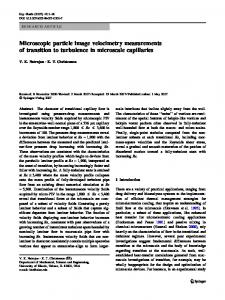
2.1 Description of case set-up Generally, a TVB, consisting of two concentric cylinders, is characterized on the basis of the rotation of one or both of the cylinders, resulting in the fluid motion due to the: 1) rotation of only the inner cylinder; 2) co-current rotation of both cylinders; and 3) counter-current rotation of both cylinders. Each of these types can be further characterized on the basis of the radius ratios of both cylinders and aspect ratio of the equipment. Radius ratio, ηrr , is the ratio of the inner cylinder radius, ri , to the outer cylinder radius, ro , or ηrr = ri /ro and aspect ratio, Γ, is the ratio of cylinder length, L, to gap width, b = ro − ri , and Γ = L/b. In addition, Taylor number and Reynolds number also play a significant role in the classification of reactors in relation to the turbulence and vortex structures that will be present. The Table 2 presents the dimensions and geometrical characteristics of TVB used in the PIV study, as shown in the Figure 2. Water at room temperature was used as the working fluid. The analytical estimations for these rotational speeds, shown in Table 3, were made using the (WENDT, 1933)’s correlation for estimating dimensionless torque-G shown in Equation 2.1, as mentioned by (LATHROP; FINEBERG; SWINNEY, 1992). These analytical estimations serve as the global estimates for this TVB configuration.

G=

3/2

 

1.45 (1−ηηrrrr )7/4 Re1.5 f or4 × 102 < Re < 104



0.23 (1−ηηrrrr )7/4 Re1.7

3/2

f or104 < Re < 105

(2.1)

44

Capítulo 2. Experimental Method - PIV

Tabela 2 – Dimensions and geometrical characteristics of the TVB used in the PIV system. Parameters Inner cylinder radius, ri Outer cylinder radius, ro Length of the reactor, L Gap width or distance between inner and outer cylinder, b Off-bottom clearance(OBC) or the height at which inner cylinder is placed above the outer cylinder, c Radius ratio, η= rroi Aspect ratio, Γ= hb Angular velocity, ω Rotational speed, N Reynolds Nº, Re= ri ω(rνo −ri ) 1/2

Taylors Nº, Ta=

ri

ω(ro −ri )3/2 ν

Value (dimensions) 100 (mm) 115 (mm) 200 (mm) 15 (mm) 0 (mm)

0.87 13.3 3.14 to 11.94 (rad/s) 30 to 114 (rpm) 4700 to17900 1825 to 6935

2.2 PIV set-up The PIV system consists of a class IV Quantel Big Sky Laser (15 Hz and λ=532 nm), FlowSense EO 16 MPixel camera (4872 × 3248) provided by Dantec Dynamics using a 60mm objective having a diaphragm aperture of f/2.8 to f/32 and a synchronization system, shown in Figure 2. The black colored internal cylinder is made of PVC, and the transparent external cylinder is made of Plexiglas. The camera was placed on the top of the TVB to the capture the motion of particles in the X-Y plane. The XY plane is chosen in order to capture the radial flow structures and radial gradients, which are assumed to be the principal components of the VEDR in a TVB. Capturing these smallest possible scales with regard to the radial gradients for a better estimation of VEDR is the main reason for the usage of the 2D PIV measurements in the X-Y plane, instead of the 3D stereographic or tomographic PIV study which would have provided the out-of-plane motion but at the expense of the spatial resolution. The first chosen location was dependent on the height at which the laser equipment can be located to illuminate the chosen X-Y plane. Once the reactor and the laser equipment were put into place in order to capture the closest feasible X-Y plane, the camera and lens were focused in that respective plane. Between the camera and the chosen X-Y plane lies the fluid above that plane, and the flat and transparent Plexiglas plate placed on the top of the reactor. As the Plexiglas plate is flat and the motion imparted by the inner rotating cylinder is purely tangential which spread radially towards the outer cylinder, the perspective error in order to capture the tangential and the radial velocity components is assumed to be negligible in this case.

2.2. PIV set-up

45

Figura 2 – PIV system consisting of the TVB, laser, camera, synchronization system and computer.

The focusing of the camera in the respective plane is the first step of calibration, which was achieved by using a quarter-circular flat plate of stainless steel with inner and outer radius one mm smaller than that of the inner and outer cylinders. The top of this plate was marked with horizontal and vertical lines one mm apart from each other forming a one mm square grid. The camera was focused on this plate and the images were saved in the computer program as calibration images. Then the second step for calibrating the images was conducted by computing a scale factor on the saved calibrated images. This scale factor was estimated by selecting two points on the saved images of the plate, and the known distance between the two points was provided. This procedure allowed the computer program to estimate the scale factor between the pixels and mm values along with the clarity of the images in that particular plane. Each further chosen location was 10 mm downwards which lead to a small decrease in the spatial resolution for each further location. The five chosen horizontal locations are between ZL = 0.725 ± 0.005 and 0.525 ± 0.005 with each approximately 10 mm apart from one another. Silver coated glass beads and fluorescent Rhodamine particles of 10 and 20 µm size, respectively, were used as seeding particles. A time-step size of 75, 75, 150, 200 and 300 µs was used for the 114, 90, 70, 50 and 30 rpm, respectively, with the laser sheet thickness of 1 mm. A total of 2500 image pairs were found to be more than sufficient for each ω at five different horizontal locations to achieve the statistical convergence of

46


Tabela 3 – Analytical estimations for the TVB used in the PIV system. Parameters Moment, τ 3/2 ηrr 1−ηrr

=

2

Gρν h, where

Value (dimensions) 114 (rpm) 90 70 50 0.022 (Nm) 0.015 0.01 0.006

30 0.003

11.9 (rad/s) 1.19 (m/s) 1.78 (N/m2 )

9.4 0.94 1.19

7.3 0.73 0.78

5.2 0.52 0.46

3.1 0.31 0.21

1.35 (N/m2 )

0.9

0.59

0.35

0.16

0.042 (m/s)

0.035

0.028

0.021

0.015

0.037 (m/s)

0.03

0.024

0.019

0.013

0.035 0.27 (Watts) 0.132 (W/kg)

0.037 0.14 0.07

0.038 0.07 0.035

0.04 0.03 0.015

0.048 0.01 0.004

52.5 (µm)

61.6

73.0

90.5

124.5

1.3 (mm)

1.4

1.5

1.7

1.9

3.172 m2 s−3

1.415

0.602

0.211

0.046

1.814 m2 s−3

0.809

0.344

0.121

0.027

7/4

G = 0.23 Re1.7 , (WENDT, 1933) Angular Velocity, ω Tip Speed, ri ω Wall shear stress at inner wall, τwi = τ /(2πri2 h) Wall shear stress at outer wall, τwo = τ /(2πro2 h) Friction q velocity at inner wall, uτ i = τwi /ρ Friction q velocity at outer wall, uτ o = τwo /ρ uτ i /ri ω Global power, P=τ ω Average VEDR, hi = P/(ρπ(ro2 − ri2 )h) Average Kolmogorov’s micro-scale, 1 hηi = (ν 3 /hi) 4 Average micro-scale, q Taylor’s 2 hΛi = 15νui /hi VEDR at inner wall, innerwall = u4τ i /ν VEDR at outer wall, outerwall = u4τ o /ν

0

0

0

0

the second order fluctuating velocity components, namely ur2 , uθ2 and ur uθ , as shown in Figure 3. The acquired data was processed with an image acquisition system provided by Dantec Dynamics, Dynamicstudio V4.0. The vector analysis was conducted using the adaptive correlation with overlapping windows ranging from 0 to 75 % and ICS ranging between 64 to 8 pixels squared for high resolution. The spurious vectors were removed using range validation, and then these were replaced by moving average validation using 3 or 5 neighboring cells, in most cases 3 neighboring cells were used. In total, less than 2.9, 3.5, 4, 7.7 and 6.7 % percent of spurious vectors were replaced at the ZL = 0.725, 0.675, 0.625, 0.575 and 0.525 ± 0.005, respectively. The spatial resolutions based on these aspects for the horizontal plan located at ZL = 0.725 ± 0.005 are presented in the Table 4.

2.3. Estimation of VEDR

47

Tabela 4 – Different ICS and overlap windows tested at ZL = 0.725 ± 0.005. ICS 64 32

16 8

Overlap window 0 0 25 50 75 0 25 50 75 0

Spatial resolution in µm 546 273 205 136 68 136 102 68 34 68

2.3 Estimation of VEDR The PIV measurements were taken in a horizontal plan in a location where U or u’ 0 = Uθ or uθ represents mean and fluctuating tangential component and V or v’ = Ur or 0 ur represents mean and fluctuating radial component of the velocity. In this context, y represents the radial directions and θ = tan−1 (y/x) represents the tangential direction, respectively, and were extracted as *.txt files from the image files using the Dantec Dynamic program Dynamicstudio V3.31. These txt files for the experimental results were treated with Matlab to create the gradients using the 2nd order central differencing approximation of the first derivative, Equation 2.2, for the central elements. The boundary elements being only at the inner and outer wall due to the usage of the 2nd order scheme were not considered for the VEDR estimation.

0

fi =

1 fi+1 − fi−1 + E, E ∼ = h2 (−fi3 ) 2h 6

(2.2)

The gradients were estimated using the mean and fluctuating velocity components using the cylindrical coordinates (SUBRAMANIAN, 2015). The VEDR derived from the gradients of the mean and fluctuating velocity components are here-onwards termed as the VEDR of the mean flow kinetic energy (MFKE) and TKE, respectively. These two components of the VEDR are estimated directly from the Equations 2.3 and 2.4, albeit only five out of 12 gradients are estimated from the PIV measurements in the x-y plane, as

48


Figura 3 – Convergence statistics of moment of order one (a) and two (b) on a horizontal plane located at ZL =0.725 and radially at Rb =0.082.

shown in Equations 2.5 and 2.6, respectively for the mean flow and turbulence components.

m =

   ν 2 

1 ∂Ur + r ∂θ

∂Ur ∂r !2

!2

1 ∂Uθ Ur + + r ∂θ r

1 ∂Uz + r ∂θ

!2

∂Uz + ∂r

!2

!2

∂Uz + ∂z

!2 

∂Ur + ∂z

!2

+

∂(Uθ /r) ∂Ur 1 ∂Uθ ∂Uz ∂Ur ∂Uz +2 + + ∂r ∂θ r ∂z ∂θ ∂z ∂r

∂(Uθ /r) r ∂r

∂Uθ + ∂z

!)

!2

!2

(2.3)

2.4. Basic Aspects of PIV

t =

     ν 2  

1 ∂u0r + r ∂θ 

49

!2

0

∂ur ∂r

!2

0

0

1 ∂uθ ur + + r ∂θ r !2

1 ∂u0z + r ∂θ

∂u0z + ∂r

0

!2

!2

∂uz + ∂z

!2

∂u0r + ∂z

!2

0



0

∂(uθ /r) r ∂r

 +

0

∂uθ + ∂z

!2

!2

(2.4)



0

∂(uθ /r) ∂u0r 1 ∂uθ ∂u0z ∂u0r ∂u0z  +2  + + ∂r ∂θ r ∂z ∂θ ∂z ∂r   

∂Ur m = ν 2  ∂r 1 ∂Ur + r ∂θ

!2

 

t =

 ν 2 

!2

1 ∂Uθ Ur + + r ∂θ r

!2 

∂(Uθ /r) + r ∂r

!2

(2.5)



∂(Uθ /r) ∂Ur  +2 ∂r ∂θ 0

∂ur ∂r

!2

0

0

1 ∂uθ ur + + r ∂θ r

!2

  +

0

∂(uθ /r) r ∂r

!2

(2.6) 0

+

1 ∂ur r ∂θ

!2

0

+2

0



∂(uθ /r) ∂ur  ∂r ∂θ

2.4 Basic Aspects of PIV Every basic choice in the utilization of PIV equipment has a significant impact on the estimation of the finer quantities, such as VEDR. To estimate accurately the smaller structures a very fine spatial resolution is required. The interesting aspect is that the actual spatial resolution is known after the treatment of data, meaning that the concentration of particles, size of particles and time-step between frames is decided by hit and trail method. In addition, all these basic aspects are inter-related to each other. This section shows the importance of these basic aspects in the estimation of the VEDR. All these aspects were studied with the 114 rpm rotational speed unless otherwise stated.

2.4.1 Concentration of particles Figure 4 shows the concentration of particles in a horizontal plane in the TVB without a grid (4a) and with a 32 grid square (4b) at two different rotational rates of 114 rpm and 30 rpm. This figure presents two aspects related to the concentration of particles: firstly, variation in the concentration with the change in rotational speed; and secondly, variation in concentration with change in ICS. It can be seen that there are lesser number of particles in the 30 rpm frame (the one in the front) in comparison to the 114 rpm (the one behind) in both parts a) and b). The reason behind this is the gradual

50


sedimentation of particles with each decrease in the rotational speed from 114 rpm to 30 rpm. An improvement in the concentration may be required in order to attain a fine spatial resolution as the rotational speed is decreased.

Figura 4 – Concentration of particles in a horizontal plane in the TVB at two different rotational rates: 114 (the one behind) and 30 (the one in front) rpm without grid (a) and with a 32 square grid (b). The choice of ICS value is directly related to the concentration of particles in the fluid. As mentioned earlier sedimentation leads to a decrease in the concentration or reduction in the number of particles in each square grid of 32 pixels with many empty grids as well. Empty grids generate spurious vectors which have to be replaced with the average of surrounding cells. This is one of the reasons behind the noise in the data; thus, poor concentration may lead to erroneous results, especially in the estimation of the smallest scales. If a smaller grid is chosen, say square grid of 16 pixels, then these empty grids will only increase requiring further substitution, in other words increasing noise in the data.


51

2.4.2 Size of particles Figure 5 presents the influence of particle size on the tangential mean velocity components and its squared fluctuating velocity component located at Zh = 0.725 ± 0.005 using a time-step of 75 µs. Clearly the reduced particle size has not only improved the tangential mean velocity component but also has a significant impact on its squared fluctuating counterpart. Though there could be a slight difference of location of ± 1 mm between the two particle size estimations, a probable reason behind slightly different profile structures. Anyhow, in terms of the mean tangential velocity component, the estimations of the 10 µm particle size were completely identical for all four of the ICS values; whereas, for the 20 µm particle size the structures for the four ICS values had some slight differences and a little bit of noise as well. The noise becomes more pronounced for the 20 µm particle size in the estimation of the squared fluctuating tangential velocity component in addition to another problem of doubling of the magnitude with each decrease in the ICS value. The magnitude increases two times when the ICS value is decreased from 64 to 32 and from 32 to 16 and so on. This increase is not practical, and this lead to this study of understanding the influence of particle size on the estimation of the flow parameters. Size of particle is important in order to attain the optimum concentration to attain a fine spatial resolution. The smallest available true spatial resolution is the one with overlap zero is 16 square grid leading to a spatial resolution of 136 µm (Table 4). An important point to note is that the 8 grid structure is actually adapted from the 16 grid structure; therefore, 16 square grid is considered as the smallest true spatial resolution available in this study. As per general guidelines, around 5 particles per square grid are considered an optimum concentration. Fitting five particles of the size of 20 µm in grid size of 136 µm is practically very difficult and may result in agglomeration of particles which will hinder further the estimation of smaller scales. Hence, based on this understanding the particle size was reduced from 20 µm to 10 µm, and a drastic improvement was seen in the estimations of squared fluctuating tangential velocity component (Figure 5b). It can be seen that the magnitude variation between the 64, 32 and 16 square grids is very small with only slight improvements in magnitude and increase in the total number of data points. Moreover, there was very little noise in the data which in comparison to the estimations of the 20 µm is practically unnoticeable. The results of the ICS 8 square grid for the 10 µm particle size were considered unpractical in similarity with the results of the 32, 16 and 8 square grid for the 20 µm particle size. The 8 square grid has a spatial resolution of 68 µm, which implies that fitting five particles of 10 µm size in 68 µm will be a challenging proposition as in the case of the 20 µm particle size. Particles of size between 2-3 µm are required in order to achieve correct estimations for the 68 µm spatial resolution. However, due to limited time and financial resources it was not possible to use extremely costly particles of mean diameter of 2-3 µm.

52


Figura 5 – Impact of particle size on the estimations of mean tangential velocity (a) and squared fluctuating velocity (b) for the horizontal plane located at Zh = 0.725 ± 0.005.


53

2.4.3 Time-step between frames First of all, time-step is the difference in the time between a double frame image. A double frame image is necessary in order to estimate the movement of particles within that time-step from the first frame to the second. Depending on the fluid flow conditions and the chosen spatial resolution, the time-step should be small enough to capture the movement of particle from the first frame to the second. As per general guidelines, the movement of particle covering 1/4th of the ICS is considered sufficient. However, when the time-step is very small of the order of 100 µs, it becomes necessary to choose time-step wisely. In this case, we studied four different time-steps within the range of 50 to 200 µs. In the Figure 6, the influence of the time-step on the mean tangential velocity and squared fluctuating velocity component is shown. As in the case of the particle size, there is practically no influence of the time-step on the mean tangential velocity component. On the other hand, in the case of squared fluctuating tangential velocity component, the impact is significant on both the noise and magnitude value. With each decrease in the time-step from 50 towards 150 µs, the noise is reduced drastically and so does the magnitude. The results for the 150 and 200 µs are very similar with little noise. These estimates of four different time-steps conducted with the 20 µm particle size were compared with the particle size of 10 µm using time-step of 75 µs, to compare with the better estimates obtained with the 10 µm particles. The estimations of the 10 µm particles were found to be very similar with the one using 150 µs time-step for the 20 µm particles. This suggests that the size of particle also plays a significant role in the determination of the time-step. The time-step size for the 20 µm particles is double that for the 10 µm particles to obtain valid results. It should be noted that the slight variation in the profile structure is most probably due to difference of location of ± 1mm between the profile structures for the two different particle sizes. To study further this effect of the particle size on the time-step, Figure 7 presents the estimations of the dimensionless VEDR of mean flow kinetic energy for the two particles sizes located at Zh = 0.725 ± 0.005. In the x and y axis of the Figure 7, the shear velocity, uτ i, and the VEDR, innerwall , at the inner wall are the analytical estimations mentioned in the Table 3. It can be seen that smaller the time-step is, higher the estimation of the VEDR becomes in the case of 20 µm particles. The squared fluctuating tangential velocity estimations for the 50 µs time-step were unpractical, and those estimations for the 150 and 200 µs time-step were of similar magnitude. However, this is not the case for the estimation of the VEDR where the 150 µ time-step estimations are higher in magnitude in comparison to those of the 200 µs time-step. On the other hand, the estimations of the 10 µm particles at 75 µs time-step are even better in the boundary layer area and the bulk

54


Figura 6 – Impact of time-step on the estimations of mean tangential velocity (a) and squared fluctuating velocity (b) for the horizontal plane located at Zh = 0.725 ± 0.005 using particle size of 20 µm.


55

Figura 7 – Influence of the time-step and particle size on the VEDR of mean flow kinetic energy. zone of the inner cylinder. This clearly demonstrates the need of the smaller time-step and particle size for improved predictions of not only the fluctuating velocity components but also the VEDR; thus, making the 10 µm particle size as the preferred choice for this study and 75 µs time-step for the 114 rpm rotational speed. Based on this rationale, time-step for the other rotational speeds was chosen.

2.4.4 Choosing overlap & ICS The interrogation cell size (ICS) value is the initial grid structure in which the flow domain is divided to obtain the velocity vectors. Smaller the ICS value is, finer the grid structure becomes generating the smallest feasible spatial resolution. To estimate the velocity vectors, the double framed image is interposed on each other to observe the movement of particle from one frame to another. When interposing the two frames if no adjacent areas are used, then it is termed as the zero overlap ratio and the spatial resolution is equivalent to the basic grid structure of the ICS. However, if the adjacent area

56


is used, usually between 25, 50 and 75 %, then the number of data points are increased for each increase in the adjacent area from 25 to 75 % leading to smaller spatial resolution for each increase in the overlap ratio. Contrary to the ICS value, higher the overlap ratio smaller the spatial resolution becomes; therefore, we see a spatial resolution of 68 µm at 32, 16 and 8 ICS with an overlap of 75, 50 and 0 respectively, as shown in the Table 4. It is important to note that the different overlap ratios use the same initial grid structure. The 64 pixels square grid at zero overlap ratio is the coarsest grid with a spatial resolution of 546 µm with least number of data points. Although, the spatial resolution of 546 µm is more than two times finer than the Average Taylor’s micro-scale of 1.3 mm, such fewer points leads to comparatively poor estimation of even the mean tangential velocity components near the inner and outer boundaries, as shown in Figure 8. A higher overlap ratio was not tested for the 64 pixels square grid due to the coarseness of the basic grid structure, and the objective of studying the smallest scales which would have been feasible only with smaller ICS values. Additionally, such fewer data points do not allow studying the boundary layer area in detail.

Figura 8 – Radial profile of mean tangential velocity at different overlap ratios and ICS values at ZL = 0.725 ± 0.005. The results for the mean tangential velocity profile becomes independent of the ICS from 32 pixels squared onwards or 273 µm; in other words, at higher ICS values the flow structure may not be the actual representation while the lower ICS values will


57

not provide any improvement in the estimation for the mean velocity components. If the estimations of the grid are independent, then the overlap ratio also should not influence the predictions of the mean tangential velocity component, which can be clearly seen in the Figure 8. The only advantage of using the overlap ratio for the estimation of the mean velocity component is to increase the number of data points in the boundary layer area, where lay the steepest gradients and could be beneficial in the prediction of the gradients of the mean flow components of the VEDR. The estimation of the squared fluctuating tangential velocity component (Figure 9) also shows slight improvement in its estimation for the smaller ICS values and for higher overlap ratios in the boundary layer area. It should be noted that the estimations for the 8 ICS pixels square grid are considered inaccurate, hence not presented in the VEDR estimations. This inaccuracy arises due to the practical impossibility of achieving a good concentration of particles of the size10 µm per square grid of 68 µm. Resulting poor concentration generates many empty grids which are replaced by the average of surrounding particles and most of the grids with only one or two particles which in turn generates poor estimation of the turbulence with a lot of noise in the data. As per general guidelines, around 5 particles per square grid are considered an optimum concentration to generate a good velocity vector. Smaller particles of the size of 2-3 µm which could have been ideal for the 8 ICS square grid were not tested due to their extremely high cost. The experimentation with 20 µm particle size lead to discovery of this error, as can been seen in the Figure 5b. The estimations for the particle size 20 µm doubled for each decrease in the ICS value from 64 to 32 to 16 to 8 due to poor concentration of particles of even bigger size in similar spatial resolutions. Additionally, the results of the 16 ICS value were found to be slightly better than those of the 32 ICS value near the walls. The estimations of the 50 % overlap were very similar to those of the 75 % near the boundary layer, and with much less noise in the bulk zone. In terms of the viscous dissipation of mean flow kinetic energy estimated from the gradients of the mean velocity components (Figure 10), an improvement can be seen in the estimation for both the overlap ratio and ICS value in the boundary layer area. An increase in the noise can be seen with increase in the overlap ratio for the 16 ICS with significant amount of noise for the overlap ratio of the 75 % in the bulk zone. The 16 ICS Overlap 75 have a spatial resolution of 34 µm, respectively, which is far too small for the particle size of 10 µm to have good concentration of particles, which consequently leads to this increased amount of noise in the estimation of the small magnitude values of the viscous dissipation of mean flow kinetic energy present in the bulk zone. The fluctuating tangential velocity component at 16 ICS Overlap 75 also presented significant amount of noise, as shown in Figure 9, which will only become worse for an even finer estimation of the VEDR; consequently, the 16 ICS Overlap 75 has not been presented for the viscous dissipation of turbulent kinetic energy estimated from the fluctuating velocity components.

58


Figura 9 – Radial profile of squared fluctuating tangential velocity at different overlap ratios and ICS values at ZL = 0.725 ± 0.005.

Interestingly, the 16 ICS Overlap 50 and 32 ICS Overlap75 have a spatial resolution of 68 µm each, respectively, but the amount of noise is much less as can be seen in Figure 11. The less noise in the 32 ICS Overlap 75 in comparison to the 16 ICS Overlap 50 indicates that higher base grid structure helps in maintaining a better concentration of particles per square grid. The prediction of viscous dissipation of turbulent kinetic energy (Figure 12) is higher for each reduction in the ICS value and increment in the overlap ratio. At the overlap ratio of zero, the magnitude increases by almost an order in the bulk zone for each decrease in the ICS value. While, for a constant ICS value, each increment in the overlap ratio predicts gradual increment in the magnitude of the viscous dissipation of turbulent kinetic energy through-out the reactor. This is the first instance where the increase in the overlap ratio has such a significant impact on the magnitude of the variable. It seems logical that with each decrease in the ICS value, smaller scales of turbulence are being captured. Tokgoz et al. (2012) also observed similar observations of continual increase in their VEDR estimation for each decrease in the ICS or IW (interrogation window) as shown in Figure 13. It can be seen that with decrease by half in the IW values, i.e. from 160 to 80 to 40 IW, of the Tokgoz et al. (2012), the increase in the estimation of


59

Figura 10 – Radial profile of the viscous dissipation of mean flow kinetic energy at different overlap ratios and ICS values at ZL = 0.725 ± 0.005. VEDR is quite significant, in similar aspect of the results presented in this study. The difference is that their magnitude values are much lower due to their much courser spatial resolution (smallest resolution of 391 µm) for similar Reynolds number, and they used the instantaneous velocity components for the prediction of their VEDR. Such gradual increase generates another question if there is still under-prediction in the estimation of the viscous dissipation of turbulent kinetic energy. To resolve this question, the impact of the spatial resolution on the viscous dissipation of turbulent kinetic energy is presented in Figure 14. The data presented in the Figure 14 is shown in the Table 5. First of all, it is important to understand the information that is being presented in the Figure 14 and Table 5. This data is presented only for one horizontal location because t,max is different at each horizontal location and will generate significant amount of noise in the data. Ideally for the purpose of statistics, a mean value of the t,max over the axial length should be considered for each and every rotational velocities at different ICS and overlap ratios, but is not possible in this case. Presently, only in the case of 16 ICS overlap 50, there is access to the mean value of the t,max over the five horizontal locations and is equal to 0.66 which is very close to the value of 0.77 located at ZL = 0.725 ± 0.005. This work was derived from the work of Delafosse et al. (2011), where they presented similar data for the stirred rank reactor and used the variable mean /N 3 D2 instead of

60


Figura 11 – Radial profile of the viscous dissipation of mean flow kinetic energy at different overlap ratios and ICS values at ZL = 0.725 ± 0.005. Tabela 5 – Dimensionless Spatial resolution,δ/hηi, for different rotational velocities, ICS values and overlap ratios located at ZL = 0.725 ± 0.005. Rotational speed, rpm 114

90 70 50

ICS 64 32 16 16 32 16 32 16 32 16

Overlap window 0 0 0 50 50 50 50 50 50 50

δ/hηi 10.4 5.2 2.6 1.3 2.2 1.1 1.87 0.94 1.5 0.75

t,max /innerwall 0.012 0.029 0.1 0.77 0.15 0.71 0.25 0.93 0.38 1.57

t,max /innerwall . t,max is used in this study because Delafosse et al. (2011) extracted the mean from the impeller discharge region where the dissipation rate is maximum and far greater the mean dissipation rate values. N 3 D2 represent the maximum value that can be achieved based on the tip of the impeller, and in similar aspect innerwall is used which represent the maximum value that can be attained on the inner boundary in the TVB. Additionally, it is important to note that the innerwall is a global average, so there will be regions in a Taylor vortex where the local value will be higher than this and other regions


61

Figura 12 – Radial profile of the viscous dissipation of turbulent kinetic energy at different overlap ratios and ICS values at ZL = 0.725 ± 0.005.

where it will be lower. Delafosse et al. (2011) described the evolution of the dissipation rate of the turbulent kinetic energy with respect to the dimensionless spatial resolution as a power law: mean /N 3 D2 = a(δ/hηi)−b , where a = 0.69 and b = 1.15 for the stirred tank reactor. Based on this rudimentary study, a similar power law is obtained for this TVB as shown in Figure 14: t,max /innerwall = a(δ/hηi)−b , where a = 0.84 and b = 1.93. In the Table 5, it can be seen that the dimensionless spatial resolution is around 1.3, 1.1, 0.94 and 0.75 for the rotational speeds of 114, 90, 70 and 50 rpm, respectively, but the t,max /innerwall is more than one only in the case of the rotational speed of 50 rpm. Considering the case that there should be several locations where the local VEDR value will be higher than the global estimate, it can be confirmed that there is still some under-estimation of the viscous dissipation of turbulent kinetic energy at higher rotational speeds, especially the 114 rpm. In terms of the percentage of under-estimation, based on the study of Saarenrinne e Piirto (2000), who stated that the dissipation rate corresponds to 90 % of the exact value if the spatial resolution is around 2η, the present study must be under-estimating by less than 10%, considering the global average value of 52.5 µm for the Kolmogorov scale (Table 3). Further refinement in the size of particles and/or technological enhancements can shed further clarity on this subject.

62


Figura 13 – Figure no 20 of Tokgoz et al. (2012) presenting dissipation rate estimations for changing interrogation window sizes (IW) for Res =14,000 with exact counter-rotation of cylinders. 75 % overalap ratio was used for all IWs.

Figura 14 – Influence of the dimensionless spatial resolution of the maximum viscous dissipation of turbulent kinetic energy estimated at ZL = 0.725 ± 0.005 for different rotational speeds at different ICS and overlap ratios. Overall, the 16 ICS square grid presented the best acceptable results among the four grids that were tested. For this grid structure, the 75 % overlap was found to present a fair amount of noise in the prediction of much finer quantities, i.e. the fluctuating tangential velocity component and the two components of the VEDR. Therefore, the 50 % overlap ratio was accepted as the chosen overlap ratio for the rest of this study. Similarly, 16 square grid was chosen as the ICS value for the rotational speed of 90, 70 and 50 rpm; whereas, for the rotational speed of 30 rpm the 32 square grid was found to be the optimum value.

2.5. Results and discussion

63

2.5 Results and discussion The results, until unless mentioned otherwise, are presented with the particles of size 10 µm at 16 ICS and 50 % overlap ratio.

2.5.1 Mean velocity flow field The tangential and radial velocity profiles at five rotational velocities are presented in Figures 15, 16, 17, 18, 19, respectively. First of all, due to a technical problem the motor became unstable at values lower than 40 rpm for the rotational speed of 30 rpm at the horizontal locations of ZL = 0.575 ± 0.005 and ZL = 0.525 ± 0.005. Secondly, 114 rpm was the highest limit of the motor which is the one and only reason for choosing this value. Kobayashi et al. (1990) presented these two components of the velocity in three regions of a Taylor-vortex in their experimental results, and observed similar flow structures. These three regions best describes the structure of a Taylor vortex pair, the extreme ends of the vortex pair, center of each vortex, and the center of the vortex pair. At the center of a vortex pair, termed as outward for describing its profile structure, the flow is moving from the inner rotating cylinder towards the outer stationary cylinder where it divides into two opposite vortexes of same size. When the flow reaches the extreme ends of each vortex pair, the flow starts diverging towards the inner rotating cylinder from the outer cylinder, hence termed as inward. Finally, each vortex of the pair has a center termed as center. The rest of profile structures lie between the outward and inward region but with profile structures similar to that of the center of vortex region, as observed by Kobayashi et al. (1990). It is very important to note that the results presented here may not necessarily show these three exact regions but the closest among the available five horizontal locations for the presented rotational velocities. In the case of mean tangential velocity, the outward region is marked by the strongest flow profile and the weakest flow profile represents the inward region. The center of vortex region is represented by the flow profile with fairly constant flow in the bulk region, Rb = 0.1 to 0.9, with a magnitude of around 50 % of the tip velocity. The strength in the outward region is imparted by the rotating inner cylinder, while the weakness in the inward region is caused by the deceleration of the fluid by the outer wall ((KOBAYASHI et al., 1990)). In the bulk zone of the center of vortex region, the magnitude of the tangential velocity increases slightly but gradually moving from the inner cylinder towards the outer cylinder. Kobayashi et al. (1990) cited that the reason behind this is the phenomenon of uniformity in the circumferential velocity induced by convection of the secondary flow. This phenomenon states that the velocity profiles apart from the ones in the outward and inward region are very similar to the one in the center of vortex region which was also observed by Kobayashi et al. (1990). Overall, in the boundary regions there is sharp

64


Figura 15 – The tangential (a) and radial (b) velocity flow profiles at 114 rpm.



65

66





67

68


Figura 19 – The tangential (a) and radial b) velocity flow profiles at 30rpm.


69

decrease in the velocity, and in the bulk zone the flow remains in the vicinity of 0.5 magnitudes, i.e. 50 % of the tip velocity. For the mean radial velocity, the outward and inward flow structures are opposite of each other represented by the upward and downward parabolic curves, respectively. While, in the center of the vortex region both of these profiles should cancel each other out and attain a zero magnitude. The center of the vortex region has been captured mostly well by all of the representing rotational velocities for both radial and tangential components of the velocity at the axial locations of ZL = 0.675, 0.675, 0.675, 0.525 and 0.725 ± 0.005 for the rotational speeds of 114, 90, 70, 50 and 30 rpm, respectively. The best inward region profiles for these two components were obtained at the 30, 50 and 70 rpm, as shown in Figures 19b, 18b and 17b at axial locations of ZL = 0.675, 0.725 and 0.625 ± 0.005, respectively; though, each at different horizontal locations, which clearly indicates variations in the height and location of the Taylor’s vortexes with the variation in the rotational speed. On the other hand, the closest profile for the outward region was captured only at the rotational speed of 114 rpm (Figure 15a) at the axial height of ZL = 0.625 ± 0.005 with a distinct second at 90 rpm (Figure 16a) also for the axial location of ZL = 0.625 ± 0.005. This poor prediction of the outward region in comparison to the inward and center of vortex region lies in the fact that there are two inward and center of vortex regions for only one outward region for each Taylor-vortex pair. This lower probability for the outward region is considered the main reason behind the absence of this region for the rotational speeds of 30, 50 and 70 rpm (Figures 19a, 18a and 17a). It is of great interest to note that the magnitude of the radial component of the velocity is only around 10 % of the tangential component (Figures 19b, 18b and 17b), in agreement with Kobayashi et al. (1990). Secondly, the steepest gradient of the tangential component velocity lie in the boundary layer area. This could imply that more than 80 % of the kinetic energy and its dissipation are represented only by the tangential component of the velocity in the boundary layer area. This aspect will be studied later on to understand the percentage impact of each of the five gradients on the VEDR. Another interesting observation is that the 80% of the cylinder width, the bulk zone, is represented by only 50 % of the magnitude of the flow with very little variation as far as the tangential component is concerned. This could turn out to be a significantly influential in terms of culturing animal cells because of similar flow conditions with very little gradients in the major part of the TVB.

2.5.2 Logarithmic velocity profiles In a Taylor-Vortex reactor, the RANS equation in cylindrical coordinates can be written as in Equation 2.7. For a steady state and assuming that the axial velocity component is negligible and the tangential velocity component depends only on the radial

70


position, the present case can be simplified to the Equation 2.8. In the center of vortex region, the radial velocity component, Ur , is negligible, which further simplifies to the Equation 2.9, and which on expansion gives Equation 2.10. From the Equation 2.10, the total viscosity, i.e. the sum of molecular and turbulent, can be extracted as shown in Equation 2.11.





2

∂Uθ ∂Ur Uθ 1 ∂Uθ 2Ur Uθ ∂Uz Uθ  ρ + + + + ∂t ∂r r ∂θ r ∂r 0

0

1 ∂P 1 ∂r2 τθr 1 ∂ρu0r u0θ 2ρu0r u0θ 1 ∂(τθθ − ρuθ2 ) 1 ∂(τθz − ρu0z uθ ) =− + 2 − − + + + ρgθ r ∂θ r ∂r r ∂r r r ∂θ r ∂z 0 0 1 ∂r2 (τθr − ρu0r u0θ ) 1 ∂(τθθ − ρuθ2 ) 1 ∂(τθz − ρu0z uθ ) 1 ∂P + 2 + + + ρgθ =− r ∂θ r ∂r r ∂θ r ∂z (2.7) 2Ur Uθ 1 ∂r2 (τθr − ρu0r u0θ ) = 2 r r ∂r

(2.8)

∂r2 (τθr − ρu0r u0θ ) = 0, or ∂r tot r2 (τθr − ρu0r u0θ ) = r2 τrθ = ri2 τrtot iθ

(2.9)

ρ

r2 (ν + ν t )r

1+

∂(Uθ /r) = ri2 u2τ i ∂r

ri2 u2τ i νt = ν r3 ν ∂U∂rθ /r

(2.10)

(2.11)

The profiles of this total viscosity at different rotational speeds is presented in Figure 20 in the center of vortex region. The limit of this simplified approach can be observed at the rotational speed of 30 rpm. It can be clearly seen that the data exhibit a similar trend which can be modeled by the Equation 2.12. νt ((r+ − ri+ )uτ i /ν)2 1+ = ν 102

(2.12)

From the Equation 2.12, an analytical expression of the velocity can be derived by injecting the non-dimensional variable, r+ = ruτ i /ν, ri+ = ri uτ i /ν and Uθ+ = Uθ /uτ i to obtain Equation 2.13. On integrating the Equation 2.13, a new equation for the mean velocity profile, Equation 2.14, is obtained with a constant C, where this constant C is found to be inversely proportional to ri+ , as shown in Figure 21. In the Figure 21, it can be


71

Figura 20 – The total viscosity at different rotational speeds in the center of vortex region. seen that the constant C= 15/ri+ , which gives us the expression of velocity in the Equation 2.15. ∂(Uθ+ /r+ ) 102 ri+2 = ∂r+ (r+ − ri+ )r+3

(2.13)

50r+ ri+ (−6r+2 + 3ri+ r+ + ri+2 ) ( Uθ+ = +2 + 6log + r+ − ri+ ) + Cr+ + +2 + r (r − ri )r ri

(2.14)

50r+ ri+ (−6r+2 + 3ri+ r+ + ri+2 ) ( + 15r+ + Uθ+ = +2 + 6log r − r ) + i r+ (r+ − ri+ )r+2 ri+ ri

(2.15)

"

"

#

#

Based on the expression presented in Equation 2.15, the logarithmic profile of the velocity is presented in Figure 22 in the center of vortex region for the four rotational speeds. The rotational speed of 30 rpm is not presented because of its poor representation of the total viscosity in the Figure 20. Clearly it can be seen that in this case, the velocity structure clearly follows the new expression of log law after the viscous sub-layer. Most of the studies (BILSON; BREMHORST, 2007; HUISMAN et al., 2013; PONCET; VIAZZO; OGUIC, 2014) regarding the logarithmic law of the wall have used the classical expression

72


Figura 21 – The evaluation of the constant C presented in the Equation 2.14. of the type u+ = 1/κln(d+) + B. Near the walls in the viscous sub-layer till d+ =10, the velocity follows a profile of u+ = d+, then there was huge buffer region till d+ =100, as mentioned by Poncet, Viazzo e Oguic (2014) and which can be observed in the study of Huisman et al. (2013). The classical expression of log-law was obeyed only after d+=100, which becomes negligible for the lower range of turbulent Reynolds no. In the present case, the log-law is obeyed as soon as the viscous sub layer is finished at d+=10. With each increase in the Reynolds number, the new log-law is obeyed better. The application of this new law at even higher Reynolds numbers, the range used in the study of Huisman et al. (2013), can prove the worth of this law.

2.5.3 Reynolds stresses 2.5.3.1 Normal stress In Figures 23, 24, 25, 26 and 27, the second order mean fluctuating components of 0 the velocity also known as Reynolds normal stresses, namely u0r2 and uθ2 are presented for the five rotational velocities at five horizontal locations apart from the rotational speed of 30 rpm, for which only three horizontal locations were available. The profile structures of 0 the Reynolds normal stresses, uθ2 and , u0r2 , presented here qualitatively coincide well with those of the Kobayashi et al. (1990). However, the magnitudes of these stresses, u0r2 and


73

Figura 22 – The log-law profile of the velocity in the center of vortex region of the inner cylinder boundary layer.

0

uθ2 , in comparison with the results of Kobayashi et al. (1990) are significantly higher in the boundary layer and at-least double in the bulk zone. The closest profile structures for the three regions, outward, inward and center of vortex region, can be observed only for 114 rpm rotational speed,as mentioned earlier. The basic difference between the profile structures for these three regions lie in the bulk zone for the normal tangential stress. In qualitative agreement with Kobayashi et al. (1990), the flow structure in the outward region is slanted decreasing gradually from the inner cylinder towards the outer cylinder and contrary in the inward region, i.e. gradually decreasing from the outer cylinder towards the inner cylinder. In the center of vortex region, the magnitude remains practically constant through-out the bulk zone. The profile structures of the center of vortex and inward regions can be seen in all of the rotational speeds (Figures 23a, 24a, 25a, 26a and 27a). The inner boundary layer of the normal tangential stress is marked by steep peaks near the wall; whereas, in the outer boundary layer the peaks are much smaller in comparison. This is the result of the fact that the maximum for the mean tangential velocity always lies on the inner cylinder with steep decreases in both boundary layers but with little variations in the bulk zone (Figure 15). Therefore, boundary layers are marked by steep gradients compared to the ones in the bulk zone.

74





75

76





77

78


Figura 27 – The tangential (a) and radial b) normal stress profiles at 30rpm.


79

The magnitude of normal radial stress, equivalent of the minimum of the normal tangential stress, is very similar in the bulk zone and the boundary layer area in the three regions, the difference is minimal. The magnitude difference among the three regions is also small but highest for the outward and inward regions and near the lowest in the center of vortex region, in qualitative agreement with Kobayashi et al. (1990). The disparity with the results of the Kobayashi et al. (1990) lies in the magnitude values for these two squared fluctuating components. Kobayashi et al. (1990) observed that the maximum of the normal radial stress is around 60 % of the normal tangential stress with the maximum 2 value for the normalized normal tangentital stress being 0.002, normalized with Utip . While, in present study the maximum normalized normal tangential stress value is more than five 2 times higher, also normalized with Utip , and the maximum of normal radial stress is less than 20 % of the normal tangential stress. Hout e Katz (2011) also presented these normal stress terms but for counter-rotating Taylor-Couette flow. It should be noted that they normalized the rms values of radial and tangential fluctuating velocities with the friction velocity instead of the tip velocity as in this case. Moreover, there range did not cover the boundary layer on the outer cylinder, and the location within the vortex at which these profiles are presented is not specified. For the normal tangential stress, they observed a similar structure as in the outward region, a peak near the inner boundary layer then gradual decrease towards outer cylinder in the bulk zone.

2.5.3.2 Shear Stress 0

Figures 28, 29a, 29b, 30a and 30b present the Reynolds shear stress, namely u0r uθ , for the five rotational velocities at five horizontal locations apart from the rotational speed of 30 rpm, for which only three horizontal locations were available. Both the magnitude 0 and the structure of the shear stress, u0r uθ , is similar to the estimations of the Kobayashi et al. (1990), but of opposite sign. The opposite sign just implies that the location of extraction of data is different. The higher magnitude of the tangential component has a significant impact on the structure of the tangential-radial shear stress term. There is a peak near the inner wall and then a gradual decay towards the outer cylinder, similarly observed in Kobayashi et al. (1990) in the outward region. In the inward region, the peak is towards the outer cylinder with a gradual decay towards the inner cylinder, and in the center of vortex region this shear stress term is of near zero magnitude through-out the bulk zone. This shear stress term was also presented by Hout e Katz (2011), and they normalized by using both the tip velocity and friction velocity at the inner cylinder. Looking at 0 there Figure 13(a) for the shear stress term u0r uθ normalized by tip velocity, a similarity can be seen in the outward flow profile of the same term at 114 rpm (Figure 28). Among

80


0

Figura 28 – The Reynolds shear stress, u0r uθ , profiles at 114rpm. the profiles for different rotational speeds, after 114 rpm only 90 rpm has these three regions distinguished. At all other rotational speeds, only center of vortex and inward region can be seen among the five horizontal locations. This is clearly a disadvantage of the experimental method with data available at very few locations in addition to the uncertainty of exact location of extraction of data.

2.5.4 Viscous energy dissipation rate 2.5.4.1 Composition of the VEDR In the Figures 31 and 32, the five gradients of the VEDR estimation of the mean flow and turbulent kinetic energy, respectively, are presented for the horizontal location of ZL = 0.725 ± 0.005. It can be clearly seen that the viscous dissipation of mean flow kinetic energy is mainly composed of only the ( ∂(U∂rθ /r) )2 gradient, while in the case of viscous 0 θ /r) 2 dissipation of turbulent kinetic energy the gradient, ( ∂(u∂r ) , is the major contributor especially in the boundary layer area, and in the bulk zone its contribution is similar to the other gradient of the radial direction. Although, there are only five gradients instead of 12 for the complete estimation of VEDR, it is known that the axial velocity is also not very strong in the Taylor- Couette flow. The impact of axial flow on the VEDR could be considered to be similar to that of the radial flow, i.e. in the bulk zone and very little


81

0

Figura 29 – The Reynolds shear stress, u0r uθ , profiles at 90 (a) and 70 (b) rpm.

82


0

Figura 30 – The Reynolds shear stress, u0r uθ , profiles at 50 (a) and 30 (b) rpm.


83

in the boundary layer. Thereby further enhancing the importance of the gradient of the tangential (both mean and fluctuating) velocity component in the radial direction in the estimation of the VEDR. In other words, capturing the propagation of the velocity in the radial direction is of utmost importance in order to estimate well the mean and turbulence components of the VEDR, especially in the boundary layer.

Figura 31 – The estimation of VEDR of mean flow kinetic energy and its 5 gradients at ZL = 0.725 ± 0.005. The estimation of the VEDR using the isotropic assumptions based on the work ∂u0θ /r) 2 of Sharp e Adrian (2001) would imply that the (( ∂r ) gradient is used 3 times, and for the axi-symmetry assumption this gradient would be used two times. Hence, we could observe a direct impact on the estimation of VEDR using these assumptions leading to an estimate which is just a multiple factor of the one with only five gradients through-out the gap-width. Just because the estimation will be higher does not necessarily means that it will be the correct estimation. The composition of the VEDR of the mean flow and turbulent turbulent kinetic energy (Figures 31 and 32) showed that using an assumption based methodology which worked in the case of stirred tank (DELAFOSSE et al., 2011) may not be as successful in other geometries. Taylor-Couette is basically a tangential flow and radial flow is only about 10 % of the tangential flow. Axial flow should also be in the range of radial flow (KOBAYASHI et al., 1990). Therefore, for better estimation it is important to know the percentage composition of each of the 12 gradients on the VEDR,

84


Figura 32 – The estimation of VEDR of turbulent kinetic energy and its 5 gradients at ZL = 0.725 ± 0.005.

afterwards a newer and simpler equation can be created for 2D PIV results. Perhaps, this can be done numerically because experimentally the estimation of all 12 gradients while capturing the smallest scales is still out of reach as shown by Tokgoz et al. (2012). There is another similarity between these two components of the VEDR, the magnitude of the gradient of radial fluctuating velocity component is same for both, radial and tangential, directions. This aspect of viscous dissipation of turbulent kinetic energy is more important as it confirms that the turbulence is not fully isotropic, and further confirmed by the fact that none of the isotropy ratios, Kijkl , are equal to 1, as shown in Figure 33. The fully isotropic hypothesis implies that the following equations (2.16, 2.17 and 2.18) of the isotropic ratios (Kijkl ) are respected (DUCCI; YIANNESKIS, 2005; DELAFOSSE et al., 2011).

0

Kjjjj =

∂uj ∂j

0

Kijij

1 ∂ui = 2 ∂j

!2

!2

0

∂uk / ∂k

0

∂uk / ∂k

!2

=1

(2.16)

= 1, i 6= j

(2.17)

!2


85

0

Kijji

0

0

∂u ∂u ∂uk = −2 i j / ∂j ∂i ∂k

!2

= 1, i 6= j

(2.18)

Figura 33 – Comparison of isotropy assumptions on radial profiles at ZL = 0.725 ± 0.005. It can be seen in the Figure 33 that none of these ratios exhibit values close to 1, in-fact most of the ratios exhibit values closer to zero. The cross product gradient, term Kijji , and the ratio Kjjjj show the maximum departure from isotropy with a mean value of 0.0047 and 0.0003, respectively. Only one of the isotropy term Kijij has a value of 0.5 in the bulk zone, the gradient of the tangential fluctuating velocity component in the radial direction; while, the other isotropy term Kijij displayed departure from isotropy with a mean value of 0.0007. As per authors knowledge, this kind of isotropic study has not been conducted before in the TVB. Though, in the stirred tank Sharp e Adrian (2001), Ducci e Yianneskis (2005), Delafosse et al. (2011) have presented work on these isotropy ratios, and there are some similarities with their work. Their cross product term also exhibited maximum deviation from the isotropy, and their term Kijij also had a value of ≈ 0.5. The difference is that their Kjjjj ratio was closer to 1 in contradiction to this study. Additionally, Ducci e Yianneskis (2005) had access to the 9 mean squared gradients through their multi-point LDA study and Delafosse et al. (2011) conducted 2D-PIV study in three different planes in order to capture all of the gradients but in different locations and spatial resolutions.

86


The spatial resolution also has a significant impact on the Kijkl ratios in complete agreement with Delafosse et al. (2011), as shown in the Figure 34. These averaged ratios were conducted on the horizontal plane located at ZL = 0.725 ± 0.005 for the various ICS and overlap ratio mentioned in Table 4. At spatial resolutions far greater than the Kolmogorov scale, the averaged value of the Kijkl ratios increases slightly, in similar observation of Delafosse et al. (2011). As mentioned by Delafosse et al. (2011), the reason behind this anomaly is that there are lesser number of data points at higher spatial resolutions which lead to comparatively higher average in comparison to the lower spatial resolutions.

Figura 34 – Variation in the Kijkl ratios influenced by the dimensionless spatial resolution for the radial profiles located at ZL = 0.725 ± 0.005. Another interesting observation is that there are two different values for the Kijkl ratios at value near to 1 of the x-axis. These two different values for the same dimensionless spatial resolutions are for the 32 ICS Overlap 75 (higher value) and 16 ICS Overlap 50 (lower value). Although, the spatial resolution obtained is same through different overlap ratios, the higher base grid structure ICS of 32 is courser than the 16 ICS and therefore captures comparatively less information. This confirms further the importance of the ICS value in relation to the overlap ratio. Main aim of the overlap ratio is to increase the number of data points. True estimation comes from the base grid structure, which presently is hindered by both cost and technological development; for example, a camera with 32 or perhaps 64 Mpixels (higher cost), not available at the time the study was conducted, will


87

provide access to double or quadruple amount of the information but will require particles of size 1 µm which are extremely costly. The advantage of this study is that the whole of gap-width is covered and at different horizontal locations similar results were obtained (results not shown) in comparison to a stirred tank where only a small area near the impeller region is studied. On the other hand, the disadvantage is that only five gradients are available in this study; thus, the Kijkl ratios are not known for the rest of the gradients. Perhaps, a validated numerical study with access to all 12 gradients can shed more light on this subject to provide more clarity on the anisotropy in a TVB. 2.5.4.2 EDR structure The VEDR of the mean flow and turbulent kinetic energy is presented in Figures 35, 36a, 36b, 37a and 37b at the five different horizontal locations for the five rotational speeds, except at the rotational speed of 30 rpm where only three horizontal locations were available. In the x and y axis of these Figures, the friction velocity, uτ , and innerwall are estimated analytically from the dimensionless torque, G, estimations of the Wendt (1933) empirical correlation (Equation 2.1) cited in Lathrop, Fineberg e Swinney (1992), as shown in Table 3. It should be pointed out again that the noise in the bulk zone in VEDR estimations of very small magnitude values is due to poor concentration at higher overlap ratios. Choosing a zero overlap results in a lesser noise but also decrease substantially the number of data points available in the boundary layer (Figure 10). The location of maxima is always very near to the wall, similarly observed by Tokgoz et al. (2012), Hout e Katz (2011) either to that of inner cylinder or outer cylinder depending upon the axial location in the Taylor-Vortex. In the outward region, the location of maxima is near the outer cylinder as shown for the rotational speed of 114 rpm at the axial location of ZL = 0.625 ± 0.005, and for the inward and center of vortex region the maxima is located near the inner cylinder, at the axial location of ZL = 0.575 and 0.675 ± 0.005, respectively for the rotational speed of 114 rpm. Among the three presented regions, the viscous wall layer is weakest in the outward region because the magnitude of the tangential velocity is strongest in this region (Figure 15a); while, the deceleration of the fluid results in the increase in the viscous wall layer. It can be seen that among the three regions, VEDR is the most dominant near the inner wall with the overall maxima located near the inner wall. McEligot et al. (2008) termed the VEDR of mean flow kinetic energy as direct dissipation and that of turbulent kinetic energy as turbulent or indirect dissipation. They presented the numerical results of the DNS model for these components in a channel flow and zero-pressure-gradient boundary layer. They found that the direct dissipation is the dominating component of the two near the wall. As the d+ increases, both the direct and

88


Figura 35 – The VEDR of the mean flow, m , and turbulent, t , kinetic energy at 114 rpm. turbulent dissipation decreases with the reduction in the direct dissipation being much more drastic in comparison to the turbulence counterpart. Between d+ = 10 and 20, the magnitude of the direct and turbulent dissipation becomes equal, and with further increase in the d+ values the direct dissipation continues decreasing much more rapidly leading to the turbulence dissipation becoming the dominating component in the bulk zone. Most of these aspects can be observed in the current estimations of these two components of the VEDR for the TVB for the five rotational speeds presented here. The only difference is that the direct dissipation is not dominating as estimated by them near the wall region, but only comparatively higher. Otherwise, increase in d+ results in decrease in both of these components of the VEDR with the decrease in the direct dissipation being more rapid in comparison to the turbulence one. Furthermore, the magnitude of the direct and turbulent dissipation becomes equal between the region d+=10 and 20, along with the progressive dominance of the dissipation of turbulent kinetic energy towards the bulk region, where turbulence component of the VEDR is at-least an order higher. In fact, in the bulk region, the direct or mean flow kinetic energy dissipation becomes practically negligible by reaching values less than 1 % of the maximum value in complete agreement with the results of McEligot et al. (2008). Turbulence takes over completely in the bulk zone once the viscous wall layer becomes negligible around d+=30 for a classical zero-pressure gradient case, as mentioned


89

Figura 36 – The VEDR profiles of the mean flow, m , and turbulent, t , kinetic energy at 90 (a) and 70 (b) rpm.

90


Figura 37 – The VEDR profiles of the mean flow, m , and turbulent, t , kinetic energy at 50 (a) and 30 (b) rpm.


91

by McEligot et al. (2008). They defined the viscous wall layer as the region with significant effects of viscosity which are not necessarily dominant and include the laminar and buffer sub-layers. The importance of this region lays in the fact that the largest gradients and greatest production of turbulence occur in this region besides being the region which provides major resistance to the momentum, mass and energy transfer (MCELIGOT et al., 2008). Additionally, it can be seen that the VEDR remains fairly constant in the viscous sublayer. These aspects of following the classical turbulence further strengthen the validity of these results. It should be pointed out again that the noise in the bulk zone in VEDR estimation is due to the choice of higher overlap. Choosing a zero overlap results in a lesser noise but also decrease substantially the number of data points available in the boundary layer, and increases the under-estimation of the turbulence VEDR due to reduction in the spatial resolution, as can be seen in the Table5. In order to capture the smallest scales, the smallest feasible spatial resolution is chosen by accepting a certain amount of noise and keeping the validity of the results. The profile structure of the VEDR for these five rotational speeds is very similar to that of the normal tangential stress (Figures 23a, 24a, 25a, 26a and 27a) at the three specified locations: outward, center and inward. First and foremost, boundary layers on both walls are marked by gradients with sharp decrease. The differentiation between the outward, center and inward region is decided by the location of the maxima, as explained earlier, and the flow structure in the bulk zone. In the bulk zone of the outward region, the flow manifests a gradual decrease from the inner cylinder towards the outer cylinder, and vice-versa for the inward region. This aspect further strengths the importance of capturing well the tangential gradient in the radial direction. The dimensionless VEDR makes its profile appear to be of similar magnitude at different rotational velocities, especially in the center of vortex region which has best prediction among the three presented regions for these five rotational velocities. In this center of vortex region, the magnitude estimation of the VEDR is comparatively higher for the 30 rpm followed by 50, 70, 90 and 114 rpms. Similar effect can be seen in the inward and outward region as well. Moreover, the magnitude of the VEDR of mean flow and turbulent kinetic energy mostly stayed ≤ 1 for the rotational velocities of 114 and 90 rpms in the three presented regions. This implies that the maximum VEDR for these two components never goes above the global estimated value, whereas global estimate is the mean of all regions where there will certainly be maximum values higher than the global estimate, as demonstrated by the rotational velocities of 50 and 30 rpms. These two aspects further indicate that there is certainly some under-prediction at higher rotational velocities. In order to use the TVB as a bio-reactor, the most important constraint will be to

92


keep the VEDR within sub-lethal responses of a cell-line in order to achieve the desired results. Godoy-Silva, Mollet e Chalmers (2009) discovered that around 60 W/kg = m2 s−3 maximum VEDR, the CHO cell line gave the sub lethal physiological responses that are critical to a bioprocess. CHO cell line is one of the most robust cell lines that exist in present time, but there are many cell lines which are much more sensitive and their sub-lethal response could be found at a much lower value. In this study, as per global estimates of the VEDR, the maximum value of 3.17 was obtained located at the inner wall for the rotational speed of 114 rpm. The maximum value is only achieved in the viscous sub-layer very near to the wall where the cells may never reach due to the nature of the viscous layer of providing resistance to any kind of transfer. Away from the wall, the VEDR decreases rapidly and its magnitude is much smaller than 1 W/kg. The animal cells are bound to spend the maximum amount of time within a Taylor-vortex in the bulk zone, between Rb = 0.1 to 0.9, where the gradients are much smaller and hold similar magnitude, i.e., similar hydrodynamic conditions in the major part of the reactor. This is a big advantage for a Taylor reactor to be used a bioreactor for culturing animal cells.

2.5.5 Kolmogorov scale In the Figure 38, the Kolmogorov scale, η = (ν 3 /)1/4 is presented for the five rotational speeds at the center of vortex region. The center of vortex region was chosen because this region was best characterized by all the presented rotational speeds. The Kolmogorov scale presented here is always smaller than the global Kolmogorov scale through-out the gap width, except for the rotational speed of 30 rpm, where the PIV estimated Kolmogorov scale was smaller only in boundary layer area. The Kolmogorov scale has significant importance for the culturing of animal cells in bioreactors. Kunas e Papoutsakis (1990) observed increase in the cell damage due to the fluid hydrodynamic forces when the Kolmogorov eddy size approaches the cell size. They conducted these experiments in the absence of the bubbles to clarify that the damage is directly related to fluid hydrodynamic forces only. At the same time, there is no proof if there is any interaction between the cells and eddies or how the cells are damaged. Although, there may not be a direct relation with the Kolmogorov scale and a certain amount of turbulence might be necessary to ensure adequate mixing and mass transfer within the bioreactor, a significant amount of turbulence is known to damage the animal cells. Smith e Greenfield (1992) managed to culture the animal cells at a Reynolds No. of 25,000 in a tank stirred with Rushton turbine at a rotational speed of 600 rpm with estimated maximum and mean VEDR of 21.8 and 0.697 m2 s−3 (SINGH, 2011), respectively, corresponding to the minimum and mean Kolmogorov scale of 15 and 35 µm. Considering these aspects and that the animal cell size ranges between 10-15 µm,

2.6. Conclusions

93

Figura 38 – The Kolmogorov scale for different rotational speeds at the center of vortex region. the range of hydrodynamics that can be employed in a bio-reactor can be ascertained to avoid damage to animal cells in suspension provided an accurate estimation of VEDR is available because the Kolmogorov scale is inversely proportional to VEDR.

2.6 Conclusions The main aim of this chapter was to present a direct VEDR estimation for the Taylor-Couette reactor at five different rotational velocities using only five of the twelve gradients required for a complete estimation. The composition of the five gradients of the VEDR of the mean flow and turbulent kinetic energy estimation was also presented. Apart from the VEDR estimation, mean radial and tangential velocity profiles, and their fluctuating counterparts are also presented in this study. In addition, a study was conducted to understand the impact of overlap ratio and ICS on the VEDR estimations, and mean and fluctuating velocity components. The overlap study showed that overlap ratio does not ameliorate the estimations of the mean and fluctuating velocity components because the base grid structure, ICS, was able to capture these components, still the overlap ratio only increase the data yield

94


for a particular ICS value. However, overlap ratios did improve on the VEDR estimations by capturing the smaller scales but at the expense of increased noise in the estimation of smaller magnitude values of the bulk zone. If there is a possibility of reaching the Kolmogorov scale with the ICS grid structure, then a zero overlap ratio could suffice. Unlike the overlap ratio, ICS plays a significant role in the estimation of even the mean and fluctuating velocity components apart from the VEDR estimations. ICS value should be chosen depending upon the requirements of a particular study; for example, requirements of VEDR implies the usage of the smallest feasible ICS value which is equivalent of or closest to the Kolmogorov scale. If only mean flow is required than the ICS value should capture at-least the Taylor’s micro-scale, but at the same time making sure that there are sufficient number of data points for a good estimation of the flow. The magnitude of radial velocity component is only around 10 % of that of tangential component, and is nearly zero in the center of vortex region. In the outward and inward regions, the maximum is achieved towards the center of the gap-width forming a downward and upward U-like shapes for the outward and inward regions, respectively. In the case of tangential velocity component, the boundary regions are marked by sharp decreases and the bulk zone is characterized by a near constant flow structure in the vicinity of 50 % of the magnitude, while being strongest and weakest in the outward and inward regions, respectively. The strong tangential flow implies that it will have a significant contribution in the kinetic energy and its dissipation, and to capture its diffusion in the radial direction from the inner cylinder towards outer implies the requirement of very small mesh in this direction, especially near the walls where lies large gradients. Similarly a steep decrease can be observed in the boundary layers of the normal tangential stress with little variation in the bulk zone in regards to the tangential component of the velocity. The center of the vortex region was best captured by the five presented rotational velocities, while the outward region was practically not captured by the 70, 50 and 30 rpm. The simple reason behind this could be the higher probability, as there are two centers of vortexes for each outward flow structure. The limited number of results that can be achieved due to practical reasons is one of the shortfalls of the experimental method. This limitation is one of the reasons for the popularity of numerical simulations, where data can be obtained anywhere within the geometry easily. The VEDR of mean flow kinetic energy is mainly composed of the ( ∂(U∂rθ /r) )2 ∂(u0 /r)

gradient, and the gradient, ( ∂rθ )2 is the major component of the turbulence VEDR especially in the boundary layer area. In addition, because of such a huge impact of only one gradient on the VEDR estimation, the application of isotropic and axi-symmetric assumptions is not valid in this case and leads to over-estimation. The dissipation of the mean flow kinetic energy was comparatively stronger in the boundary layer area, while the dissipation of turbulent kinetic energy was at-least an order higher than its mean

2.6. Conclusions

95

flow counterpart in the bulk zone. The profile structures of these two components of VEDR in the three aforementioned regions for the five rotational velocities were observed to be very similar to the normal tangential stress again citing the significance of the tangential velocity component in the estimation of and turbulence VEDR. Knowing that this VEDR estimation is based on only five gradients, and considering that the axial velocity component has a similar impact as that of the radial velocity component, it becomes necessary to capture well the propagation of tangential velocity component in the radial direction, especially in the boundary layer for a better estimation of both components of VEDR. These experiments were conducted with a view to validate numerical results, especially the VEDR estimations which contain the smallest scale. If the smallest scales of numerical results can be validated, than those results can be used with 100 % confidence leading to better designs and operating conditions. Therefore, the next chapter focuses on the validation of the numerical results with more attention towards the boundary layer area where lie the steep gradients. Another important aspect of the numerical simulations will be to estimate the VEDR using all the 12 gradients and presenting the compositions of those 12 gradients in order to better deduce an equation to estimate the VEDR from 2D PIV results.

97

3 Numerical Method and its Validation All of these simulations were performed on a desktop with six-core and twelve-thread 3.5 GHz i7-3970X processor, and 64 GB of memory. All of the simulations were run using hpi based parallel processing with 4 cores. The CFD software Fluent of ANSYS-Fluent (2010) version 13.0.0 was used to perform the numerical simulations in the TVB used for the PIV estimations. The details of the TVB can be seen in the Table ??, as shown in the Chapter 2. In this section, firstly the basic numerical aspects used in the TVB model will be presented, along with a brief description of the turbulence models used in this study. Then the numerical model will be validated with the experimental results presented in the Chapter 2 at one of the PIV horizontal location for the rotational speed of 114 rpm. The analytical estimations for the TVB at 114 rpm can be found in the Table ??, Chapter 2. Only the DNS model will be used for the validation of the numerical model.

3.1 Turbulence modelling Turbulence, a time and space varying fluctuations in the flow field, is a phenomenon of three dimensional structures and unsteady nature made up of various scales, and characterized by Reynolds number. It is generated when the inertial forces overpower the viscous forces. Navier-Stokes equations for continuity, momentum and energy are used to describe both the laminar and turbulent flows. Present simulations are conducted in isothermal state, so the energy equation is not required here. In addition, it is assumed that the flow is incompressible, fluid is Newtonian and there are no external forces; thus, the Navier-Stokes equations for continuity (Equation 3.1) and momentum (Equation 3.2) become: ∂ui =0 ∂xi

(3.1)

 ∂ui ∂(ui uj ) 1 ∂p ∂ ∂ui ∂uj     + =− + ν + ) ∂t ∂xj ρ ∂xi ∂xj ∂xj ∂xi

(3.2)

In order to solve all the spatial and temporal scales of the turbulence a direct numerical simulation (DNS) of the Navier-Stokes equations (3.1 and 3.2) has been conducted; though, to resolve all the scales the computational mesh must confirm to the 3 smallest dissipative scales known as the Kolmogorov scale, given by, η = ( ν )1/4 . If the computational mesh is not fine enough, a certain amount of information will be lost

98

Capítulo 3. Numerical Method and its Validation

depending upon the coarseness of the mesh. The details of the computational mesh are discussed in the following section. Although, the DNS can resolve all the scales if the computational mesh is fine enough, it is known to be the most time and computational resource consuming model (BARTELS et al., 2002). Considering that the mesh may not be fine enough to resolve all the scales and in order to reduce the time and computational resource consumption, the LES turbulence models may be considered as a viable option. LES model is based on the assumption that basically large eddies result in the transfer of the momentum, mass, energy and other passive scalars. Therefore, the governing equations of the LES model are obtained by spatially filtering over small-scales. Eddies with scale smaller than the filter are eliminated and are modeled with a sub grid scale (SGS) model. The SGS model describe the interaction between the resolved and unresolved scales (BAKKER; OSHINOWO, 2004). The application of a filtered variable (Equation 3.3) for an LES model in the Navier-Stokes equation leads to new unknown quantities in the momentum Equation 3.4. The filtered variable is denoted by overbar, in the Equation 3.3, where D is the fluid domain and G is the filter function which determines the scale of the resolved eddies. In the Equation 3.4, τij represents the SGS stresses and is the unknown quantity that arose out of the filtering process. In the Ansys Fluent, the SGS stresses τij are correlated to the large-scale tensor Sij (Equation 3.5) using eddy viscosity approach as shown in Equation 3.6. f¯(x) =

Z

f (x0 )G(x; x0 )dx0

(3.3)

D

 ∂ u¯i ∂ u¯j  ∂τ ∂ u¯i ∂(u¯i u¯j ) 1 ∂ p¯ ∂   − ij + =− + ν + ) ∂t ∂xj ρ ∂xi ∂xj ∂xj ∂xi ∂xj

(3.4)

1  ∂ u¯i ∂ u¯j     Sij =  + 2 ∂xj ∂xi

(3.5)



τij − −

δij  = 2νSGS S¯ij τkk  3

(3.6)

The νSGS is the subgrid scale eddy viscosity representing the smaller scales. There are various LES models available in the Fluent and each is differentiated from the other based on its definition of this SGS eddy viscosity. In this study, as mentioned earlier, two LES models are used, namely the Smagorinsky and wall adapting local eddy-viscosity (WALE) models. The Smagorinsky LES model describes this SGS eddy viscosity as shown in Equation 3.7, where LS = min(κd, CS ∆) is the mixing length for SGS, where κ is the von Kárman constant, d is the distance to the closest wall, CS =0.2 is the Smagorinsky constant and ∆ is the local grid scale and computed as power 1/3 of the volume of the

3.1. Turbulence modelling

99

computational cell. In the case of the the WALE model, the SGS eddy viscosity is described in the Equation 3.8, where LS = min(κd, CW ∆) with the CW = 0.325 being the Wale constant.

¯ |S| ¯ ≡ νSGS,Smag = L2S |S|,

q

2S¯ij S¯ij

(3.7)

(Sijd Sijd )3/2 νSGS,W ALE = L2S ¯ ¯ 5/2 , (Sij Sij ) + (Sijd Sijd )5/4

(3.8)

2 2 Sijd = 1/2(g¯ij2 + g¯ji ) − 1/3δij g¯kk , g¯ij = ∂ u¯i /∂xj

Apart from the DNS and LES models, the four RANS based models, namely k-, SST, SAS-SST and RSM, used in this study are derived from Reynolds-averaging of the underlying Navier-Stokes equations (3.1 and 3.2) for an Newtonian fluid and incompressible flow. This process introduces Reynolds stresses, −ρui uj , in the momentum Equation 3.9 that have to be modelled to form a closed system of equations. In the Equation 3.9, p0 = p + 2/3k is the modified pressure and νef f = ν + νt , where νt is the turbulent viscosity that arose out of the averaging process and must be modelled. In the case of LES model, the filtration process introduced the SGS eddy viscosity representing the smaller scales which needed to be modeled. In the two equation RANS based model, turbulent viscosity is introduced based on the Boussinesq hypothesis, but the difference is that the turbulent viscosity represents all of the turbulent scales in contrast to only the small scales for the LES models. This approach of the RANS based models impact both the reliability of the modelled equations and the computational cost required to solve them.  ∂ui ∂(ui uj ) 1 ∂p0 ∂ ∂ui ∂uj    νef f  + =− + + ) ∂t ∂xj ρ ∂xi ∂xj ∂xj ∂xi

(3.9)

In two-equation models, the Boussinesq hypothesis is used to model the unknown Reynolds stresses by assuming they can be approximated by the product of the mean strain rate multiplied by an isotropic turbulence viscosity. There are a variety of models that have been formulated but here we focus on just two of them. Firstly, the k- model, based on transport equations for the turbulent kinetic energy, k (Equation 3.10), and the turbulence energy dissipation rate, (Equation 3.11), is used in which the turbulent viscosity is described as νt = Cµ k 2 /. In these equations, Gk = νt S 2 represents the generation of turbulent kinetic energy due to the mean velocity gradients, and the value for the model constants C1 , C2 , Cµ , σk and σ is 1.44, 1.92, 0.09, 1.0 and 1.3, respectively. Whilst this model has known limitations, particularly its unsatisfactory performance in the near-wall

100


region, it is still very widely used and also provides a good starting point to generate an initial flow field for more complicated models. ∂k ∂(kui ) ∂  νt  ∂k   ν +  + = +Gk − ∂t ∂xi ∂xj σk ∂xj

(3.10)

∂  ∂ 2 νt  ∂ ∂(ui )   ν +  + = +C1 Gk − C2 ∂t ∂xi ∂xj σ ∂xj ρk k

(3.11)

The k- model employs wall functions as the equations cannot be integrated to the wall. In order to address this problem, models in which the turbulence energy dissipation rate is replaced by the turbulence eddy frequency, ωtef , have been derived. These behave well near the wall and allow the detailed behavior inside the boundary layer to be calculated. However, they perform poorly away from walls due to a problem with over-sensitivity to the free stream conditions. Menter (1994) blended the k- and k-ω models and added a turbulence production limiter in the calculation of the eddy viscosity (Equation 3.12) to produce the now widely used Shear Stress Transport (SST) model. It provides accurate predictions of the onset and the amount of flow separation under adverse pressure gradients (MENTER, 1994).

νt =

1 k ω max 1 , SF2 a∗

(3.12)

α1 ω

∂  νt  ∂k ∂k ∂(kui )   ν +  + = +min(Gk , 0.9kω) ∂t ∂xi ∂xj σkSST ∂xj

(3.13)

∂ω ∂(ωui ) ∂  νt  ∂ω min(Gk , 0.9kω)a∞ 2(1 − F1 ) ∂k ∂ω   ν +  + = + + (3.14) ∂t ∂xi ∂xj σωSST ∂xj νt ωσω,2 ∂xj ∂xj

In the Equation 3.12, the S is the magnitude of strain rate, k represents the transport equation for the turbulent kinetic energy (Equation 3.13), ω represents the transport equation for the turbulence eddy frequency (Equation 3.14), a∗ =1 for high Reynolds number, α1 is a constant of value 0.31, and F2 is a blending function (Equation 3.16), respectively. In the Equation 3.13, the σkSST = 1/(F1 /σk,1 + (1 − F1 )σk,2 ) where F1 is a blending function (Equation 3.15), σk,1 = 1.176 and σk,2 =1.0. In the Equation 3.14, the σωSST = 1/(F1 /σω,1 + (1 − F1 )σω,2 ) where σω,1 = 2.0 and σω,2 =1.168, and a∞ is ∗ defined in the Equation 3.17, where βi,1 =0.075, βi,2 =0.828, κ=0.41 and β∞ =0.09. √

F1 =

  min max  tanh 

4 k 500µ  4ρk  ,  , , 2  0.09ωy ρy ω σω,2,Dω+ y2

(3.15)

3.1. Turbulence modelling

101

Dω+ = max

F2 =



 a∞ = F1 

2ρ ∂k ∂ω , 10−10 ωσω,2 ∂xj ∂xj

   tanh max

√ 2 2 k 500µ   , 2  0.09ωy ρy ω

(3.16)

   κ2 κ2 βi,1 β   +(1 − F1 )   i,2 − q q − ∗ ∗ ∗ ∗ β∞ β σω,1 β∞ σω,2 β∞ ∞

(3.17)

A key failing of unsteady two equation models is that they cause excessive damping of turbulence and thus do not resolve any of the details of the turbulence directly (MENTER, 2009). Menter e Egorov (2010) introduced the SAS-SST to overcome this deficiency. The SAS-SST model (SAS stands for Scale Adaptive Simulation) uses a turbulence length-scale, which induces "LES-like"behavior in unsteady regions of the flow field. By adjusting the turbulence length-scale to the directly resolved turbulent structures, the eddy viscosity is reduced to the level of the limiting LES model. In this way, the model does not dissipate directly-resolved turbulent structures as classical RANS would (MENTER; EGOROV, 2010; MENTER et al., 2010). This is obtained by the addition of QSAS (Equation 3.18) term in the transport equation for the turbulence eddy frequency (Equation 3.14) of the SST turbulence model, where L is the length scale of the modeled turbulence, Lvk is the von Karmen length scale, S is the scalar invariant of the strain rate tensor Sij , and the constants η2 , C and σΦ are 3.51, 2 and 2/3, respectively.



 QSAS = max η2 κS 2 

2 L  2k 1 ∂ω ∂ω 1 ∂k ∂k   −C max 2 , ,0 Lvk σΦ ω ∂xj ∂xj k 2 ∂xj ∂xj

(3.18)

Another drawback of eddy-viscosity RANS based models is the assumption of an isotropic turbulence viscosity, which limits the development of anisotropy in the Reynolds stresses. RSM remove this assumption and solve transport equations for each of the Reynolds stresses. The model is much more computationally intensive than two-equation models and suffers from poor convergence behaviour (AUBIN; FLETCHER; XUEREB, 2004). Just as there are many variants of the two equations models, there are a large number of Reynolds stress models that differ in their closure relationships, especially for the pressure-strain term. Here the linear pressure strain variant of the model, known as the Launder Reece Rodi - Isotropization of production (LRR-IP) (LAUNDER; REECE; RODI, 1975), is used. The momentum equation for the RSM model (Equation 3.19) is similar to the one based on the Boussinesq hypothesis (Equation 3.9), but for the pressure term, p00 = p + 2/3µ∂ui /∂xk and the Reynolds stresses, ui uj , which were replaced by the νt term. These stresses are modeled as shown in the Equation 3.20, where CS−RAN S =0.22, δij ,

102


Pij and Φij are the kronecker delta, VEDR of TKE, production term and pressure strain correlation, respectively. The production term and VEDR of TKE are represented by the Equations 3.21 and 3.22, and the pressure strain correlation, where Φij = −(C1RSM ρ(ui uk − 2/3δij k)/k + C2RSM (Pij − 2/6deltaij Pij )) where C1 = 1.8 and C2 =0.6. In the Equation 3.22, the C1RSM = 1.45, C2RSM =1.9, σRSM = 1.1  ∂ui ∂(ui uj ) 1 ∂p00 ∂ ∂(ui uj ) ∂ui ∂uj    − + =− + ν + ) ∂t ∂xj ρ ∂xi ∂xj ∂xj ∂xi ∂xj

∂  2 k2  ∂(ui uj ) ∂(ui uj ) ∂(uk (ui uj )     + − = Pij − δij + Φij ν + CS−RAN S ∂t ∂xk ∂xk ∂xj 3

Pij = ui uk

∂Uj ∂Ui − uj uk ∂xk ∂xk

∂ ∂(uk ) νt  ∂ ∂      ν+ + (ρC1RSM (Pk + Pb ) − C2RSM ) + = ∂t ∂xk ∂xk σRSM ∂xk ρk

(3.19)

(3.20)

(3.21)

(3.22)

A key limitation of two-equation models is their insensitivity to streamline curvature and rotation, which is the main motivation for the use of Reynolds stress models. Recently, a modification to the two-equation models has been developed by Smirnov e Menter (2009) based on the work of Spalart e Shur (1997). This has shown considerable benefit in applications where highly swirling flows have been modelled. Singh, Fletcher e J. (2011) have shown that the addition of curvature correction to the turbulence models improves its predictions. In view of this study, curvature correction was applied to all of the two-equation turbulence models used in this study.

3.2 Numerical methodology 3.2.1 Geometry and Meshing aspects Workbench was used to construct geometry and the sweep mesh which consists of the hexahedral nodes. In view of the intended use of the DNS and LES models, and multiple reference frame (MRF) technique in the modeling aspects, a full geometry was modeled containing only one body. However, in order to obtain better control over the radial mesh, the TVB geometry was designed as a semi-circle, as shown in Figure 39, and was later on duplicated to model the full geometry. MRF technique was used instead of the more sophisticated but time-consuming sliding grid technique because the fluid movement in the TVB is only due to the inner-rotating cylinder; thus, avoiding the usage of a inner and outer geometrical configuration required for the sliding grid interface.

3.2. Numerical methodology

103

Figura 39 – Geometry and mesh of the TVB used in the PIV experiments. Table 6 shows the different parameters that were varied and corresponding node and mesh sizes. Thee maximum aspect ratio value increased from 15.9 to 32.2 to 53.6 as the number of nodes were increased only in the radial direction in terms of radial divisions of 45 in Fine to 90 in Fine2X to 150 in Finer, respectively. Although, the aspect ratio increased significantly, the orthogonal quality remained the same for each mesh type with a value of 0.9999, where values close to 1 indicate good quality. Only the 3rd Mesh name was tested for the DNS model, while all of these were tested for the LES-WALE model. In this grid-independence study, basically, the refinements in the mesh were done only in the radial direction because it is understood that the flow is radially transferred from the inner rotating cylinder to the outer cylinder, while the secondary vortices consisting of the radial and axial components of the velocity are only 10 % of the tangential component (KOBAYASHI et al., 1990). Thus, clearly citing the importance of a very fine grid in the radial direction in order to capture the smallest scales. Mesh in the radial direction was created in such a way that the nodes are smallest near the inner and outer walls and biggest in the center of the gap width. Figure 40 shows the impact of the refinements in the radial direction on the velocity flow field and TKE. Tabela 6 – Mesh configurations used to model the TVB. Mesh name Fine Fine2X Finer

No of divisions

No of nodes

Z

X

Y

millions

200 200 200

45 90 150

320 320 320

2.944 5.889 9.712

Z mm 1 1 1

Mesh size X min. X max. µm µm 156 623 79 307 47 184

Y mm 1.13 1.13 1.13

In terms of the global estimate of Taylor’s micro-scale, hΛi = 1.3 mm (Table 3), all presented mesh types are sufficiently fine both near the walls and in the bulk zone to

104


Figura 40 – Comparison of different grid sizes for the DNS and LES models of dimensionless mean axial velocity (a), radial velocity (b), tangential velocity (c) and mean square of fluctuating tangential velocity (d) axially at Rb =0.067. The legend is same in all figures.

capture the large-eddies defined by the Taylor’s micro-scale. When a much courser grid (Fine grid with 2.9 million nodes) was used with the LES-WALE model, seven vortex pair appears instead of six vortex pairs for finer grids; considering that one vortex pair is represented by two crests and one trough. Among the Fine2X and Finer grid for the LES-WALE model, the three velocity components, radial, axial and tangential, are equally well predicted when compared with the DNS model using Finer grid. However, in the case of squared fluctuating tangential velocity the Fine2X grid comparatively over-predicts, thereby enhancing the choice of the finer grid LES-WALE model to be used in the rest of article for validation purposes and a much thorough comparison with the DNS model. In addition, the Finer grid must be capturing at-least 90 % of the dissipation rate near the boundary layer, especially considering the fact that nodes near the wall are ≈ 47 µm which is smaller than the global estimate of Kolmogorov scale, hηi=52.5 µm (Table 3).

3.2. Numerical methodology

105

3.2.2 Pre-processing aspects As mentioned in the previous section, the DNS, two LES models, namely Smagorinsky and WALE, and four RANS based models, namely, k-, SST, SAS-SST and RSM were used to estimate the flow and turbulence characteristics in the TVB. The Convergence criteria of 10−4 , which was achieved within a maximum of 40 iterations per time-step, for root mean square (RMS) scaled residuals was employed for the continuity, momentum and turbulence quantities. Double precision arithmetic was applied for all of the simulations. In order to collect the data, an xz-plane was created, and a certain number of variables, including velocity components and gradients, were chosen to be extracted at the end of each time-step in the text file format. The high resolution and second order backward Euler schemes were used to model the advection and transient terms, respectively, for all the equations.

3.2.3 Solver & Post-processing aspects It took around 15 revolutions for the DNS and 5 revolutions for the LES models to achieve the moment stabilization, and 36 hours to complete one revolution for the DNS model and 24 hours to complete one revolution for the LES models. Once the moment stabilization was achieved, the data was collected for at-least 20 revolutions. The collected data was then treated using the Matlab program to process the results. As in the case of the experimental results, the statistical convergence of the second order fluctuating 0 0 0 0 velocity components, namely ur2 , uθ2 and ur2 uθ2 was also tested, and 20 revolutions or 7200 time-steps were found to be more than sufficient for an ensemble average.

3.2.4 Estimation of VEDR The numerical results, the axial, radial and tangential velocity and direction components were extracted at each time step in the *.txt format. These txt files were treated with Matlab to create the gradients using the 2nd order central differencing approximation of the first derivative, Equation 2.2, for the central elements. The boundary elements being only at the inner and outer wall due to the usage of the 2nd order scheme were not considered for the VEDR estimation. The gradients were estimated using the mean and fluctuating velocity components, as in the case of the PIV estimations and termed as the VEDR of mean flow and turbulent kinetic energy, respectively. These two components of VEDR are estimated directly from the Equations 2.3 and 2.4, respectively, in the case of DNS and LES models. Whereas, in the case of PIV measurements only five out of 12 gradients are estimated, as mentioned in Chapter 2, from the x-y plane for the VEDR of mean flow and turbulent kinetic energy, as shown in Equations 2.5 and 2.6, respectively.

106


3.3 Validation of the computational model The validation of the numerical results was done at only one of the five available horizontal locations (ZL =0.725 ± 0.005) of the PIV measurements. The comparison with the PIV data was conducted for the tangential and radial velocity components, the log-law profiles at the inner and outer boundary layers for the tangential component, squared fluctuating tangential velocity and the five available gradients of the VEDR of the mean flow and turbulent kinetic energy for the PIV measurements, as shown in Figures 41, 42,43 and 44. First of all, because the PIV location is not 100 % certain, the numerical horizontal location was chosen by observing a complete Taylor-Vortex pair and thereby choosing the most similar profile to that of the PIV measurement. The PIV profile lies in between the center of vortex and outward flow region of a Taylor-Vortex, but in close proximity to the center of vortex. The term center of vortex means as it says and the outward flow region means the region when the flow direction is at its strongest from the inner cylinder towards the outer cylinder, which is the center of a Taylor-vortex pair not to be confused with center of vortex. Each Taylor-vortex pair has one Outward flow, which lies in the center of this Taylor-vortex pair, two center of vortexes, in each vortex of the pair, and two inward flow regions, at each extremity of the pair. Secondly, considering that the numerical mesh spacing is of 1 mm in the axial direction, Figures 41a and 41b present data at two axial location for the numerical DNS model. Thirdly, the classical log-law is presented here and not the new law to validate the numerical results because the new law should be employed in the center of vortex region where the radial velocity component is practically negligible, and the chosen PIV height is nearer to the inward region instead of the center of vortex region. Finally, in the Figure 44 innerwall = u4τ i /ν, q where uτ i = τ /(ρ2πri2 h), is estimated using the DNS moment data. The tangential velocity component (Figure 41a) is well predicted by the DNS model especially in the boundary layer; in addition, the difference between the axial heights is negligible which implies that this coarseness of mesh spacing in the axial direction has little impact on the tangential velocity component. In the bulk zone, between Rb =0.1 to 0.9, in agreement with Bilson e Bremhorst (2007), the numerical model does not accompany the phenomenon of small and steady increase through-out the bulk zone, as in the case of experimental results (SMITH; TOWNSEND, 1982; KOBAYASHI et al., 1990) and Figure (41a), but only till Rb =0.4. Kobayashi et al. (1990) stated that this phenomenon is because of uniformity in the circumferential velocity, in which the velocity profiles apart from the ones in the outward and inward region are very similar to the one in the center of vortex region, which in turn is caused by convection of the secondary flow. In-fact, none of the numerical studies (CHUNG; SUNG, 2005; BILSON; BREMHORST, 2007; PIRRO; QUADRIO, 2008; PONCET; HADDADI; VIAZZO, 2011; OGUIC; VIAZZO; PONCET, 2013; FRIESS; PONCET; VIAZZO, 2013) demonstrated the capability of

3.3. Validation of the computational model

107

Figura 41 – Validation of the numerical DNS model with the PIV results of dimensionless mean tangential (a) and radial (b) velocity components.

108


Figura 42 – Validation of the numerical DNS model with the PIV results of the log-law profiles for the tangential component at the inner (a) and outer (b) boundary layers. The κ = 0.4 and B = 5.2 is used in the log profile.

3.3. Validation of the computational model

109

Figura 43 – Validation of the numerical DNS model with the PIV results of dimensionless mean squared fluctuating tangential velocity component.

the various numerical models to capture this phenomenon exhibited by experimental methods. In the case of the radial component, though the magnitude is less than 3 % of the tangential component and the shape is well predicted by the numerical model, the maximum difference between the two axial heights is approximately 25 %. In order to better capture the radial component reduction in the axial mesh size to 0.5 or perhaps to 0.25 mm is required, implying doubling or quadrupling, respectively, the total number of nodes, which is impractical presently to implement with the available computational resources and, in turn, time. The log-law profiles for the inner (Figure 42a) and outer (Figure 42b) boundary layers shows different behavior from each other. Both inner and outer velocity profiles are normalized with appropriate uτ , which is estimated from the global torque estimations of the numerical model, and for the PIV estimations, as there is no experimental torque data available, the DNS estimations are used. It should be remembered that uτ is the average of the whole axial domain and not local, which can cause imperfect matching (HUISMAN et al., 2013). As mentioned by Huisman et al. (2013), the velocity profile follows u+=d+ in the viscous sub-layer (1 λ3 , then the new definition implies that within the vortex λ2 < 0. The details of this method can be seen in the original article of Jeong e Hussain (1995) and also in the PhD thesis of Escudie (2001). 2

2

The λ2 -definition method has been used to compare the different turbulencs models with the DNS model through Figures 46, 47 and 48. To keep the number of figures in check, the secondary vortex pair for other models has not been shown here. Instead, the λ2 -definition method will help in a better comparison of these secondary vortexes in terms

116

Capítulo 4. Turbulence models

Figura 45 – Identification of the Taylor’s vortexes through λ2 (a) and a pair of secondary Taylor’s vortexes (b) for the DNS model.

4.2. Mean velocity flow field

117

of their size and structure for the presented turbulence models. For the DNS model, all vortexes but the ones on the bottom and top of cylinders are of similar size, here size refers to the value of λ2 , and structure. The vortexes on the top and bottom of the cylinders are opposite of each other in terms of the magnitude of λ2 ; The one on the bottom is of the smallest magnitude whereas the one on the top has the highest magnitude among all of the vortexes. There are six pair of vortexes in the gap width of 15 mm and height of 200 mm, leading to approximately double the size of gap-width for each vortex pair. The LES-WALE, k-, RSM and SAS-SST turbulence models also present six pair of vortexes; while, the LES-Smagorinsky and SST turbulence models presents 5 and 7 number of vortexes, respectively. This means that in comparison to the DNS model, the width of a Taylor vortex pair will be thicker for the LES-Smagorinsky model and thinner for the SST model. In-fact, for the LES-Smagorinsky model the width of each vortex pair is equivalent of 40 mm, where all vortex pairs are of practically same size (Figure 46b). In all other turbulence models, the size and structure of the top and bottom vortex pairs is different from the rest of the vortex pairs. The RSM turbulence model presents the worst comparison with the DNS model for the size, structure and magnitude values. Apart from the top and bottom vortex pairs, the λ2 magnitude value remains around 400 for the DNS and LES models. In the case of the k-, SST and RSM model, there is huge variation in the magnitude values most probably caused by the excessive damping of turbulence by the RANS based models (MENTER, 2009). An improvement can be seen in the SAS-SST model, where the turbulence length-scale is improved by adjusting it to the directly resolved turbulence structures (MENTER; EGOROV, 2005).

4.2 Mean velocity flow field 4.2.1 Tangential velocity The tangential component of the mean velocity is presented in the Figures 49, 50 and 51 at or closest to the outward, center of vortex and inward regions of a Taylor-vortex for the different numerical models. Kobayashi et al. (1990) and Bilson e Bremhorst (2007) also presented these three components in the above mentioned regions of a Taylor-vortex in their experimental, using a Pitot tube, and numerical-DNS results, respectively, and observed similar flow structures. The tangential flow is at its strongest in the outward region where the rotating inner cylinder imparts momentum to the flow to move from the inner cylinder towards the stationary outer cylinder. Whereas, in the inward region the flow is at its weakest due to deceleration of the fluid in the outer wall where the fluid is transported by convection (KOBAYASHI et al., 1990).

118


Figura 46 – Identification of the Taylor’s vortexes through λ2 for the LES-WALE (a), and LES-Smagorinsky (b) models.


119

Figura 47 – Identification of the Taylor’s vortexes through λ2 for the k- (a) and RSM (b) models.

120


Figura 48 – Identification of the Taylor’s vortexes through λ2 for the SST (a), and SAS-SST (b) models.


121

Figura 49 – Radial profiles of the tangential velocity component near the outward region of a Taylor vortex.

Figura 50 – Radial profiles of the tangential velocity component near the inward region of a Taylor vortex.

122


Figura 51 – Radial profiles of the tangential velocity component near the center of vortex region of a Taylor vortex.

An interesting point to observe is that the tangential component of the velocity is at-least 70 % of the total flow considering that the maxima for both axial and radial components is only around 15 % of the mean flow. The PIV experimental results in accord with Kobayashi et al. (1990) showed that both axial and radial components achieved a maximum of only around 10 % of the flow. Moreover, the steepest gradients for the tangential velocity lie in the boundary layer. This could imply that in the boundary layer more than 70 % of the kinetic energy and its dissipation must be represented by only the tangential component of the velocity and its gradients. Hence, for a better estimation of the kinetic energy and its dissipation requires finest grid structure on the radial direction to capture the propagation of tangential flow in-between the cylinders, especially in the boundary layers. Among the different turbulence models, the worst comparison with the DNS model was for the LES-Smagorinsky model. It over-predicted the magnitude in the outward region and under-predicted in the inward region. In all the three regions, the LES-WALE model reproduced extremely well the profile structures and magnitudes estimated by the DNS model followed by the SAS-SST and SST model with very similar predictions. The predictions of the k- and RSM model were comparatively poor in the outward and inward region in comparison to the other RANS based models. In the center of vortex region where all turbulence models predicted similar structures, the RSM model was comparatively


123

under-predictive in the bulk zone. The radial profile of the tangential component showed that within 80 % of the gap-width between Rb = 0.1 to 0.9, the magnitude of the velocity is constant at around 50 %. This aspect is of great consequence because in the case of animal cell cultures, the cell lines within the TVB will spend most of the time in the vicinity of these values of similar and weak magnitude, and only a fraction of its times will be spent near the high gradients located near the wall. Additionally, the viscous layers in the region of high gradients near the wall will further propel the cell cultures towards the bulk zone having uniform flow.

4.2.2 Radial velocity The radial component of the mean velocity is presented in the Figures 52, 53 and 54 at or closest to the outward, center of vortex and inward regions of a Taylor-vortex for the different numerical models. Kobayashi et al. (1990) observed that the axial and radial velocity components achieved a maximum of only around 10 % of the mean flow, whereas in this study and in Bilson e Bremhorst (2007)’s work a maximum of approximately 15 % for these two components is achieved. The radial velocity achieves this maximum in parabolic shapes in the outward, in the upward direction, and inward regions, in the downward direction. The upward and downward parabolic shapes of the radial velocity are due to opposite direction of flow in the outward and inward region, respectively. In the outward region, the flow is from the inner cylinder towards outer and vice-versa in the inward region. As in the case of the tangential velocity, the estimations of the LES-Smagorinsky models were over-predictive in comparison to the rest of the models in the outward and inward region. While, the RSM models estimations were under-predictive in these two regions. The LES-WALE model captured extremely well the flow structure exhibited by the DNS model followed by the SAS-SST, SST and k- models. In the center of vortex region, the radial velocity is near zero for all the turbulence models.

4.2.3 Axial velocity In the Figures 55, 56 and 57, the axial component of the mean velocity is presented at or closest to the outward, center of vortex and inward regions of a Taylor-vortex for the different numerical models. It should be noted that the structure of the axial velocity is opposite to that presented in the research work of Kobayashi et al. (1990). The reason is that the single vortex from which the data is represented in these results is from the vortex with anti-clockwise rotation, whereas the data was taken from the vortex rotating in clockwise direction by Kobayashi et al. (1990). The rotation direction of the vortex can be judged by the shape of the axial velocity in the center of vortex region, as explained by

124


Figura 52 – Radial profiles of the radial velocity component near the outward region of a Taylor vortex.

Figura 53 – Radial profiles of the radial velocity component near the inward region of a Taylor vortex.


125

Figura 54 – Radial profiles of the radial velocity component near the center of vortex region of a Taylor vortex. Kobayashi et al. (1990). In the axial velocity flow, the maximas lie near the walls, one of positive magnitude and another negative, in the center of vortex region, and in the bulk zone there is a linear distribution slanting from the positive to the negative maxima. If the positive maxima lies near the inner cylinder, then the rotation is clockwise otherwise its anti-clockwise. In complete agreement with Kobayashi et al. (1990) and Bilson e Bremhorst (2007), the axial velocity is nearly zero in both the outward and inward regions. As the axial velocity is near zero in the outward and inward region, all turbulence models estimations were similar. The small differences between these models for the small magnitude values is most probable due to the poor grid structure of 1 mm in the axial direction. The LES-Smagorinsky model was over-predicting in the center of vortex region, while the RSM model was under-predicting. Again the LES-WALE model best captured the DNS estimations followed by the SAS-SST, SST and k- model.

4.2.4 Log law profiles of tangential velocity In order to better understand the boundary layer, the classical log-law profiles for the inner (Figure 58a) and outer (Figure 58b) boundary layers are presented for the mean of the whole axial domain of the tangential velocity component. Both inner and outer velocity profiles are normalized with appropriate uτ , which is estimated from the global torque estimations of each respective numerical model. As mentioned in Chapter 3, it

126


Figura 55 – Radial profiles of the axial velocity component near the outward region of a Taylor vortex.

Figura 56 – Radial profiles of the axial velocity component near the inward region of a Taylor vortex.


127

Figura 57 – Radial profiles of the axial velocity component near the center of vortex region of a Taylor vortex.

should be remembered that uτ is the average of the whole axial domain and not local, which can cause imperfect matching (HUISMAN et al., 2013). As mentioned by Huisman et al. (2013), the velocity profile follows u+=d+ in the viscous sub-layer (199; imag=strcat(file,000,num2str(num),.txt); end

79 80

if num>999;

195

imag=strcat(file,00,num2str(num),.txt); end

81 82 83

fid1 =

84

fopen(imag,r);

85

[a b x y u v st] = textread(imag, %f%f%f%f%f%f%f,headerlines,6); % headerlines,6 tells matlab not to read first six lines because those % are just text and not data.

86 87 88 89 90

%Matrix of velocity vector is created

91

for j=1:NX for k=1:NY i=(j-1)*NY+k; U(j,k,num)=u(i); V(j,k,num)=v(i); St(j,k,num)=st(i); end end

92 93 94 95 96 97 98 99 100

status=fclose(fid1);

101 102 103

end

104 105

save Data_champs Tot NX NY Y X U V St -v7.3

106 107 108 109 110 111 112 113 114 115 116 117 118 119

% Initialising of vectors UmeanCM=zeros(NX,NY); VmeanCM=zeros(NX,NY); uflucCM=zeros(NX,NY,Tot); vflucCM=uflucCM; uflucFM=zeros(NX,NY,Tot); vflucFM=uflucFM; u2CM=uflucFM; v2CM=u2CM; uvCM=u2CM; u2meanCM=zeros(NX,NY); v2meanCM=zeros(NX,NY); uvmeanCM=zeros(NX,NY);

120

% 122 % 123 % 124 % 121

Calculating the averaged velocity components by neglecting the modified vectors, and thus considering only the vectors that were actually present in the PIV grid and neglecting the vectors which were estimated as the mean of the neighbours. These vectors are termed as CM in the end

125 126 127

for j=1:NX for k=1:NY

196

APÊNDICE A. Matlab File

Ind(j,k)=0; for num=1:Tot if St(j,k,num)==0 Ind(j,k)=Ind(j,k)+1; UmeanCM(j,k)=UmeanCM(j,k)+U(j,k,num); VmeanCM(j,k)=VmeanCM(j,k)+V(j,k,num); end end UmeanCM(j,k)=UmeanCM(j,k)/Ind(j,k); VmeanCM(j,k)=VmeanCM(j,k)/Ind(j,k);

128 129 130 131 132 133 134 135 136 137

end

138 139 140

end

141 142 143

%Similarly calculating the fluctuating velocity components by neglecting %the modified vectors.

144 145 146 147 148 149 150 151 152 153 154 155 156 157 158 159 160 161 162 163 164 165

for j=1:NX for k=1:NY Ind1(j,k)=0; for num=1:Tot if St(j,k,num)==0 Ind1(j,k)=Ind1(j,k)+1; uflucCM(j,k,num)=U(j,k,num)-UmeanCM(j,k); vflucCM(j,k,num)=V(j,k,num)-VmeanCM(j,k); u2CM(j,k,num)= uflucCM(j,k,num)* uflucCM(j,k,num); v2CM(j,k,num)= vflucCM(j,k,num)* vflucCM(j,k,num); uvCM(j,k,num)= uflucCM(j,k,num)* vflucCM(j,k,num); u2meanCM(j,k)=u2meanCM(j,k)+u2CM(j,k,num); v2meanCM(j,k)=v2meanCM(j,k)+v2CM(j,k,num); uvmeanCM(j,k)=uvmeanCM(j,k)+uvCM(j,k,num); end end u2meanCM(j,k)=u2meanCM(j,k)/Ind1(j,k); v2meanCM(j,k)=v2meanCM(j,k)/Ind1(j,k); uvmeanCM(j,k)=uvmeanCM(j,k)/Ind1(j,k); end end

166

save Data_meanCM Tot NX NY X Y UmeanCM VmeanCM u2meanCM v2meanCM uvmeanCM 168 save Data_flucCM Tot NX NY X Y uflucCM vflucCM u2CM v2CM uvCM -v7.3 167

169

%Calculating the mean of all of the vectors over the total number of time %steps, and termed as FM in the end 172 UmeanFM=mean(U,3); 173 VmeanFM=mean(V,3); 170 171

174

197

175 176 177 178 179 180 181 182 183 184 185 186 187 188

%Calculating the fluctuating velocity components of all of the vectors % for i = 1:Tot uflucFM(:,:,i)=U(:,:,i)-UmeanFM(:,:); vflucFM(:,:,i)=V(:,:,i)-VmeanFM(:,:); end % u2FM=uflucFM.*uflucFM; v2FM=vflucFM.*vflucFM; uvFM=uflucFM.*vflucFM; u2meanFM=mean(u2FM,3); v2meanFM=mean(v2FM,3); uvmeanFM=mean(uvFM,3);

189

save Data_meanFM Tot NX NY X Y UmeanFM VmeanFM u2meanFM v2meanFM uvmeanFM 191 save Data_flucFM Tot NX NY X Y uflucFM vflucFM u2FM v2FM uvFM -v7.3 190

192 193

% tests if the results are acceptable (makes sense) or not 195 n_figure=n_figure+1; 196 figure(n_figure) 197 toto=reshape(UmeanCM,NX*NY,1);hist(toto,50) 194

198

n_figure=n_figure+1; figure(n_figure) 201 toto1=reshape(VmeanCM,NX*NY,1);hist(toto1) 199 200

202

n_figure=n_figure+1; figure(n_figure) 205 tata=reshape(u2meanCM,NX*NY,1);hist(tata,50) 203 204

206

n_figure=n_figure+1; 208 figure(n_figure) 209 tata1=reshape(v2meanCM,NX*NY,1);hist(tata1,50) 207

210

n_figure=n_figure+1; 212 figure(n_figure) 213 tata2=reshape(uvmeanCM,NX*NY,1);hist(tata2,50) 211

214 215

% From these figures we choose the data that is between the inner and outer 217 % cylinder walls, neglecting the rest 216

218

Ynew=Y((34:133),(16:241)); 220 Xnew=X((34:133),(16:241)); 221 Unew=U((34:133),(16:241),:); 219

198

222 223 224 225 226 227 228 229 230 231 232 233 234 235 236 237 238 239 240 241 242 243

Vnew=V((34:133),(16:241),:); Stnew=St((34:133),(16:241),:); Umoynew=UmeanCM((34:133),(16:241)); Vmoynew=VmeanCM((34:133),(16:241)); uflucnew=uflucCM((34:133),(16:241),:); vflucnew=vflucCM((34:133),(16:241),:); u2new=u2CM((34:133),(16:241),:); v2new=v2CM((34:133),(16:241),:); uvnew=uvCM((34:133),(16:241),:); u2meannew=u2meanCM((34:133),(16:241)); v2meannew=v2meanCM((34:133),(16:241)); uvmeannew=uvmeanCM((34:133),(16:241)); UmoyFMnew=UmeanFM((34:133),(16:241)); VmoyFMnew=VmeanFM((34:133),(16:241)); uflucFMnew=uflucFM((34:133),(16:241),:); vflucFMnew=vflucFM((34:133),(16:241),:); u2FMnew=u2FM((34:133),(16:241),:); v2FMnew=v2FM((34:133),(16:241),:); uvFMnew=uvFM((34:133),(16:241),:); u2FMmeannew=u2meanFM((34:133),(16:241)); v2FMmeannew=v2meanFM((34:133),(16:241)); uvFMmeannew=uvmeanFM((34:133),(16:241));

244 245 246 247 248 249 250 251 252 253 254 255 256 257 258 259 260 261 262 263 264 265 266 267 268

Ycut=Ynew; Xcut=Xnew; Ucut=Unew; Vcut=Vnew; Stcut=Stnew; UmeancutCM=Umoynew; VmeancutCM=Vmoynew; uflucCutCM=uflucnew; vflucCutCM=vflucnew; u2cutCM=u2new; v2cutCM=v2new; uvcutCM=uvnew; u2meancutCM=u2meannew; v2meancutCM=v2meannew; uvmeancutCM=uvmeannew; UmeancutFM=UmoyFMnew; VmeancutFM=VmoyFMnew; uflucCutFM=uflucFMnew; vflucCutFM=vflucFMnew; u2cutFM=u2FMnew; v2cutFM=v2FMnew; uvcutFM=uvFMnew; u2meancutFM=u2FMmeannew; v2meancutFM=v2FMmeannew;


199

269

uvmeancutFM=uvFMmeannew;

270 271

NXcut=133-34+1; 273 NYcut=241-16+1; 272

274 275 276 277 278 279 280 281 282 283

Totcut=Tot; %%%%%%%%%%%%%%%%%%%%%%%%%%%%%%%%%%%%%%%%%%%%%%%%%%%%%%%%%%%% % saving all the data in seperate files in order to keep a small size, % otherwise a single file may become 100s of Gigabytes save Data_champscut Totcut NXcut NYcut Ycut Xcut Ucut Vcut Stcut save Data_meanCCM UmeancutCM VmeancutCM u2meancutCM v2meancutCM uvmeancutCM save Data_fluccutCM uflucCutCM vflucCutCM u2cutCM v2cutCM uvcutCM save Data_meanCFM UmeancutFM VmeancutFM u2meancutFM v2meancutFM uvmeancutFM save Data_fluccutFM uflucCutFM vflucCutFM u2cutFM v2cutFM uvcutFM

284 285

%% In this section, the VEDR of Mean flow kinetic energy is estimated

286

%%%%%%%%%%%%%%%%%%%%%%%%%%%%%%%%%%%%%%%%%%%%%%%%%%%%%%%%%%%%%%%%% % Program for the treatment of the PIV data %%% 289 % Written by Harminder Singh on July 2013 %%% 290 %%%%%%%%%%%%%%%%%%%%%%%%%%%%%%%%%%%%%%%%%%%%%%%%%%%%%%%%%%%%%%%%% 287 288

291 292 293 294 295 296 297 298 299 300 301

% we have velocity as radial and tangential components, so we have % to generate VEDR in cylindrical co-ordinates as % VEDR=mu*(2(durdrsq+(1/rduthdth+ur/r)2+duzdzsq)+(rd(uth/r)dr+1/rdurdth)2+ % (1/rduzdth+duthdz)2+(durdz+duzdr)2 % % r is radial direction with changing gradients in meteres Y=Ycut(1,:); X=Xcut(:,1); L=length(Y); C=length(X);

302

th=atan((Xcut./1000)./(Ycut./1000)); 304 r=Ycut; 303

305 306 307 308 309 310 311 312

dth=zeros(C,L); % for i=2:C for j=1:L dth(i,j)=(-th(i,j)+th(i-1,j)); end end

313 314 315

dr=(r(1,3)-r(1,1))/1000; % Radial gradient and equivalent of 2*dr

200

316


Ra=r;

317

durdthmf=zeros(C,L); 319 duthdthmf=durdthmf; 320 durdrmf=durdthmf; 321 duthdrmf=durdthmf; 318

322 323 324

for j=2:C for i=2:L-1

325 326 327 328 329 330 331 332 333

durdthmf(j,i)=(VmeancutFM(j,i+1)-VmeancutFM(j,i-1))./(2.*dth(j,i)); duthdthmf(j,i)=((UmeancutFM(j,i+1)-UmeancutFM(j,i-1))./(2.*dth(j,i))) ./Ra(j,i)+VmeancutFM(j,i)./Ra(j,i); durdrmf(j,i)=(VmeancutFM(j,i+1)-VmeancutFM(j,i-1))./dr; duthdrmf(j,i)=(((UmeancutFM(j,i+1)./Ra(j,i+1))-(UmeancutFM(j,i-1) ./Ra(j,i-1)))./dr).*Ra(j,i); end end

334 335

save Data_MeanGrad durdthmf duthdthmf durdrmf duthdrmf -v7.3

336

durdthduthdrmf=durdthmf.*duthdrmf; durdthsqmf=durdthmf.^2; 339 durdrsqmf=durdrmf.^2; 340 duthdthsqmf=duthdthmf.^2; 341 duthdrsqmf=duthdrmf.^2;

337

338

342

save Data_MeanGradSq durdthduthdrmf durdthsqmf durdrsqmf duthdthsqmf 344 duthdrsqmf -v7.3 343

345

nu=1e-06; 347 VEDRmf=nu*(2*(duthdthsqmf+durdrsqmf)+meandurdthsqmf+duthdrsqmf+2*durdthduthdrmf); 346

348

save Data_VEDRMF VEDRmf 350 %% Now, the turbulence VEDR is estimated 349

351

%%%%%%%%%%%%%%%%%%%%%%%%%%%%%%%%%%%%%%%%%%%%%%%%%%%%%%%%%%%%%%%%% 353 % Program for the treatment of the PIV data %%% 354 % Written by Harminder Singh on July 2013 %%% 355 %%%%%%%%%%%%%%%%%%%%%%%%%%%%%%%%%%%%%%%%%%%%%%%%%%%%%%%%%%%%%%%%% 352

356

durdthT=zeros(C,L,Totcut); 358 duthdthT=durdthT; 359 durdrT=durdthT; 360 duthdrT=durdthT; 357

361 362

for j=2:C

201

for i=2:L-1

363 364 365 366 367 368 369 370 371 372

durdthT(j,i,:)=(vflucCutFM(j,i+1,:)-vflucCutFM(j,i-1,:))./(2.*dth(j,i)); duthdthT(j,i,:)=((uflucCutFM(j,i+1,:)-ufluc_CutFM(j,i-1,:))./(2.*dth(j,i))) ./Ra(j,i)+vflucCutFM(j,i,:)./Ra(j,i); durdrT(j,i,:)=(vflucCutFM(j,i+1,:)-vflucCutFM(j,i-1,:))./(dr); duthdrT(j,i,:)=(((uflucCutFM(j,i+1,:)./Ra(j,i+1))-(uflucCutFM(j,i-1,:) ./Ra(j,i-1)))./(dr)).*Ra(j,i); end end

373 374 375

save Data_FlucGrad durdthT duthdthT durdrT duthdrT -v7.3

376

durdthduthdrT=durdthT.*duthdrT; durdthsqT=durdthT.^2; 379 durdrsqT=durdrT.^2; 380 duthdthsqT=duthdthT.^2; 381 duthdrsqT=duthdrT.^2;

377

378

382 383

save Data_FlucGrad durdthduthdrT durdthsqT durdrsqT duthdthsqT duthdrsqT -v7.3

384 385 386 387 388 389 390

mdurdthsqT=mean(durdthsqT,3); mduthdthsqT=mean(duthdthsqT,3); mdurdrsqT=mean(durdrsqT,3); mduthdrsqT=mean(duthdrsqT,3); mdurdthduthdrT=mean(durdthduthdrT,3);

391 392

save Data_FlucGradM mdurdthsqT mduthdthsqT mdurdrsqT mduthdrsqT mdurdthduthdrT

393 394

nu=1e-06; 396 TEDR=nu*(2*(mduthdthsqT+mdurdrsqT)+mdurdthsqT+mduthdrsqT+2*(mdurdthduthdrT)); 395

397 398

save Data_TEDR TEDR

399 400

%%

203

Índice Chine hamster ovary, 33 Computational fluid dynamics, 37 Direct numerical simulation, 39 Interrogation cell size, 37 Large eddy simulation, 39 Laser Doppler anemometry, 37 Mean flow kinetic energy, 47 Multiple reference frame, 102 Off-bottom clearance, 44 Particle image velocimetry, 37 Reynolds averaged Navie-Stokes, 39 Reynolds stress model, 39 Root mean square, 105 Scale adaptive simulation, 40 Shear stress transport, 40 Sub grid scale, 98 Taylor vortex bioreactor, 33 Turbulent kinetic energy, 39 Visocus energy dissipation rate, 34 Wall adapting local eddy, 40