Leap Frog Scheme. Physical. Figure 1: Numerical phase velocity for a wave propagating along a coordinate axis vs. grid resolution. The physical phase velocity ...
Proceedings of EPAC 2004, Lucerne, Switzerland
PARTICLE-IN-CELL BASED BEAM DYNAMICS SIMULATIONS T. Lau, E. Gjonaj and T. Weiland, Institut f¨ur Theorie Elektromagnetischer Felder Technische Universit¨at Darmstadt Schloßgartenstraße 8, D-64289 Darmstadt, Germany
Discrete Phase Velocity
Abstract Several methods for the suppression of spurious noise in the field solution, typically emerging in long-time ParticleIn-Cell (PIC) simulations, are investigated. The results are compared with the analytical solution for a bunch in a semi-infinite waveguide. As a realistic example simulations for the RF-Gun installed at Photo Injector Test Facility in DESY Zeuthen (PITZ) are presented.
1 Leap Frog Scheme Physical
0,9 0,8 0,7 0,6 2
6 10 14 Grid Points / Wave Length
18
INTRODUCTION Figure 1: Numerical phase velocity for a wave propagating along a coordinate axis vs. grid resolution. The physical phase velocity is scaled to unity.
In modern accelerator structures the dimensions of a bunch are typically much smaller than those of the geometry. This requires from an efficient numerical method to use a minimal number of grid points to achieve a given accuracy. Especially, for traditional numerical schemes the simulation of ultra-relativistic electron bunches is problematic. Time growing spurious oscillations, in the numerical field solution can totally mask the physical field. Theoretically, this oscillations can be reduced by increasing the number of grid points. Unfortunately, for most practical calculation this is not feasible, because of memory limitations. Thus, it is necessary to find efficient algorithms which eliminate this oscillations, while still retaining an accurate field solution.
NOISE REDUCTION The spacial discretization of the Maxwell equations results in an ODE system, which in the standard implementation are evaluated in time using a Leap Frog (LF) scheme, � � � � � � �� (n+1) (n) 0 h h = ALF � n+ 1 + ∆t � �(n+1) 3 �(n+ 2 ) M−1 j e e( 2 ) ε
with � ALF =
FINITE INTEGRATION TECHNIQUE The numerical method considered in this paper, for the solution of the Maxwell equations, is the Finite Integration Technique (FIT) [2]. As starting point, the integral form of the Maxwell equations on a computational grid G and it’s � are considered. Within the frameassociated dual grid G work of the FIT method this equations are casted into a set of matrix equations, � �
�
Sb = 0 C� e =−
d� � b dt
�� S d=q � d� � � �� C h = d + j. dt
The discrete material relations are given by � �
d = Mε � e
� �
�
b = Mµ h
where two positive definite matrix operators M ε and Mµ are introduced. Higher order, boundary conformal material operators resulting in a more accurate approximation of the fields have been proposed in [6].
1 −∆tM−1 µ C −1 � −1 � C∆tM ∆tMε C 1 + ∆t2 M−1 ε µ C
�
which is a second order accurate time stepping method. Fig. 1 shows the discrete phase velocity and it is seen that for waves resolved with to few grid points a very large deviation from the physical phase velocity occurs. The unphysical propagation of this unresolved waves leads to the oscillations described in the introduction. A remedy is to damp this wavelengths, which can be achieved by applying dissipative integration schemes. As dissipative algorithm, the Transversal Current Adjustment (TCA) scheme [3] was chosen in this work. The algorithm makes a slight modification of the LF method by adding an artificial damping term to suppress unresolved, short wavelengths: � � � � � � �� (n+1) (n) 0 h h = ATCA � n+ 1 + ∆t � �(n+1) 3 �(n+ 2 ) M−1 e e( 2 ) ε j with
170
ATCA = ALF − α∆t2
� � −1 � Mµ CM−1 ε C 0 . 0 0
Proceedings of EPAC 2004, Lucerne, Switzerland The dissipation parameter, α, is a free parameter and has to be chosen to an appropriate value. Depending on the value of the parameter α, the maximal stable time step for the TCA scheme is reduced in comparison with the LF method. A different approach is to improve the dispersion properties for waves propagating along the beam axis. This approach is based upon the observation, that for the field of a relativistic bunch in an accelerator structure the shorter wave lengths propagate in the longitudinal direction rather than in the transversal ones. This motivates to split the discrete curl operator, acting on the electromagnetic fields, in the numerical method into a longitudinal and a transversal part with respect to the bunch motion. The fields are updated according to the flow chart in Fig. 2 in a step by step manner by considering the transversal and longitudinal part of the curl operator respectively. A Strang splitting scheme [5] of the operators is applied to obtain second order accuracy in the time integration. The splitting algorithm, �
�(n+1)
h �(n+1) e
�
� = AS ∆t + 2
with
� AS (∆t) = AT
h
e �
+ 0
Leap Frog Update - Transversal -
Current Update -
� �(n+1)
AL (∆t)AT
∆t 2
�
applies the two-step LF scheme in each sub step. In contrast to the one-step LF method, the fields of the two-step LF method � � � � ∆t ∆t AL/T (∆t) = UL/T VL/T (∆t)UL/T 2 2 � � −1 1 −∆tMµ CL/T UL/T (∆t) = 0 1 � � 1 0 VL/T (∆t) = � ∆tM−1 1 ε CL/T
SIMULATION OF THE PITZ GUN
are allocated at the same time level. For waves propagating along the longitudinal direction at a time step equal to c0 ∆t = ∆x, the numerical phase velocity of the splitting scheme is identical to the physical phase velocity. Hence, this time step is applied in all simulation with the splitting scheme.
ANALYTICAL BENCHMARK For a rotational symmetric bunch, propagating with a constant velocity through a semi-infinite waveguide, the Green’s function is calculated in [1]. In order to compare the different numerical schemes, a bunch with a radial hatprofile in space and a truncated gaussian current distribution in time is taken. Then the analytical solution is obtained by a convolution of this profile with the greens function. For all simulations a damping parameter α = 0.02
∆t 2
in the TCA scheme was used. The computational mesh is held constant, corresponding to a resolution of 7 grid points within the bunch length. The simulation is stopped when the distance between the bunch and the source reaches the longitudinal distance of 9 cm. The simulated longitudinal electrical field on the axis of the wave guide is plotted in Fig. 3. The LF scheme shows unphysical oscillations. In comparison, the dissipative TCA scheme removes the oscillations in the vicinity of the bunch. The operator splitting scheme shows no spurious oscillations and the field in the vicinity of the bunch is more accurate than the one obtained by the other methods. If the grid resolution is increased to 14 grid points per bunch length, all schemes converge to the analytical solution.
�
�
∆t 2
Figure 2: Flow chart of a single field update for the proposed splitting scheme.
�(n) −1 � ∆t 2 Mε j
�
∆t 2
Leap Frog Update - Longitudinal - ∆t
M−1 ε j
∆t 2
∆t 2
Leap Frog Update - Transversal -
�
�(n) �(n)
Current Update -
As a realistic application for the schemes the PITZ RFgun [4] is chosen. In this structure the beam is accelerated in a 1.5 cell copper cavity operated in the π-mode at 1.3 GHz. The accelerating RF-field and the static magnetic field were computed with the computational packages CST MWS and CST EMS [7]. In the 3D-dimensional PIC simulations the external fields are added to the space charge fields. The bunch profile is a homogeneous disc in the radial direction and a flat-top function in time for the current distribution. The simulations were stopped at a longitudinal distance of 20 cm from the cathode. The simulation parameters are given in Tab. 1 and the simulation results are shown in Fig. 4. The LF scheme shows large oscillations. In comparison, the TCA algorithms is able to damp most of the oscillations, except for those in the vicinity of the bunch. The operator splitting scheme shows less oscillations than the
171
Proceedings of EPAC 2004, Lucerne, Switzerland Table 1: PITZ Simulation Parameters Beam Parameter Value Bunch Radius r0 = 1.5/mm Bunch Charge Q = −1.0/nC Bunch Length t FWHM = 20.0/ps Rise/Fall Time trise = 2.0/ps Reference Phase ϕ0 = −47.0ø Field at Cathode ECath = −40.0/(MV/m)
0,9 Analytical
Ez / (MV/m)
Leap Frog
0 Bunch
-0,9 4
6
8
10
z / cm
Pitz-Gun Geometry
0,09
0,9 Analytical Ez / (MV/m)
Ez / (MV/m)
TCA
0
Leap Frog 0 Bunch
Bunch
-0,09 10
-0,9 4
6
8
10
z / cm
18
22
TCA Ez / (MV/m)
Splitting Scheme Ez / (MV/m)
22
0,09
Analytical
0
0 Bunch
Bunch -0,09 10
-0,9 6
18 z / cm
0,9
4
14
8
10
14 z / cm
z / cm
0,09 Splitting Scheme Ez / (MV/m)
Figure 3: Longitudinal electric field on the axis of the semiinfinite wave guide for the different schemes. others, especially in the vicinity of the bunch.
0 Bunch
SUMMARY AND CONCLUSIONS
-0,09 10
Three time integration schemes based on the conformal FIT discretization are compared with respect to their ability to integrate the space charge fields, created by a relativistic bunch, in an accelerator structure. In contrast to the standard LF scheme, the TCA algorithm and the proposed splitting scheme are able to reduce the HF noise in the field solution significantly. This ability is important for the beam dynamics simulations.
14
18
22
z / cm
Figure 4: The longitudinal electric field on the axis of the PITZ RF-gun for the different schemes. [3] J. Eastwood, “The virtual particle electromagnetic particlemesh method”, Comp. Phys. Com., Vol. 64, pp. 252-266, 1991. [4] R. Cee, M. Krassilnikov, S. Setzer, T. Weiland, “Beam dynamics simulations for the PITZ RF-gun ”, PAC 2002.
REFERENCES [1] I. N. Onishchenko, D. Yu. Sidorenko, and G. V. Sotnikov, “Structure of electromagnetic field excited by an electron bunch in a semi-infinite dielectric-filled waveguide”, Phys. Rev. E, Vol. 65, pp. 665, 2002. [2] T. Weiland, “Time domain electromagnetic field computations with Finite Difference-Methods”, Int. J. Num. Mod., Vol. 9, pp. 259-319, 1996.
[5] G. Strang, “On construction and comparison of difference schemes”, SIAM J. Numer. Anal., Vol. 5, pp. 506-516, 1968. [6] B. Krietenstein, P. Thomas, R. Schuhmann, and T. Weiland, “Facing the big challenge of high precision field computation”, in Proc. 19th LINAC Conf., Chicago, IL, USA, 1998. [7] CST GmbH, “User’s Guide”, Bad Nauheimer Str. 19, D64293 Darmstadt, Germany.
172