Nov 5, 1984 - Received 16 July 1984. Revised manuscript received 10 September 1984. The dynamics of two harmonically coupled sofid bodies connected ...
Volume 105A, number 8
PHYSICS LETTERS
5 November 1984
PARTICLES ON A STRING: TOWARDS UNDERSTANDING A QUANTUM MECHANICAL DIVERGENCE ~ H. DEKKER Physics Laboratory TNO, P.O. Box 96864, The Hague, The Netherlands
Received 16 July 1984 Revised manuscript received 10 September 1984
The dynamics of two harmonically coupled sofid bodies connected to a finitely extended mechanical field (string) is solved exactly and expfieitly in the Lagrange formalism. For infinite length of the strings the particles motion becomes damped, but not as a simple linearly damped harmonic oscillator. The model allows for a detailed discussion of its quantum mechanics, in particular of a previously recognized ultraviolet divergence.
1. Introduction. Historically, our present investigations have grown out of interest in the phenomenon of dissipation. In particular in a quantum mechanical context that phenomenon appears to be quite fascinating [ 1 ]. The problem is definitely nontrivial there, mainly because quantum theory relies basically on the hamiltonian formulation o f mechanics. Dissipation can not readily be implemented in that formulation. Originally the emphasis of our research has been on the so-called phenomenological approach, especially by means of a complex variables quasi-hamiltonian theory (e.g. refs. [ 1 - 3 ] ) . Although this approach can be pushed quite far [4], the more basic problem of a proper understanding of the transition from reversible to irreversible behaviour of dynamical (sub-)systems is obviously not solved in this way. In ref. [1] we presented an investigation of a very simple model that can be solved exactly and that is rele. rant to this basic problem. It consisted of one harmonic oscillator coupled to a semi-infinite transmission line or string. Both a point mechanical and an electrical circuit system were shown to underly this model (see also refs. [5,6]). The oscillator was observed to be linearly damped in precisely the simplest textbook manner (see e.g. ref. [7]) only if essentially (i) the transmission line
a Part of a poster presented at the "Quantum noise in macroscopic systems" Conference at ITP, Santa Barbara (2127 June 1984).
0.375-9601/84/$ 03.00 ©Elsevier Science Publishers B.V. (North-Holland Physics Publishing Division)
could be considered as a continuum (material or electrical) and (ii) its length A were infinite. The first condition allows for a complete separation ~ la d'Alembert of so-called "outgoing" and "incoming" waves. The second condition prevents the reflection of "outgoing" into "incoming" waves at the far end of the line ,1 Even though the classical solutions for the above described system require a Finite renormalization of the initial conditions, apl~arently due to the fact that the model does not posses an intrinsic cut-off frequency ,2, the emerging physical picture seems quite satisfactory. However, the oscillator's quantum mechanical momentum fluctuations could not be evaluated to give a Finite result since the pertinent integral involved a logarithmic ultraviolet divergence. The calculation in ref. [1 ] anticipated the limit A -~ oo at an early stage, but in ref. [11 ] it was shown that this divergence is an exact consequence of the model for any length of the strings. It has been suggested that the origin of the troubles was to be found in the coupling between the oscillator and the string being too strong (e.g. refs. [ 9 - I 1]), in a sense to be elaborated in the present article. But the model to be discussed here differs enough from the previous one ,1 It also makes the eigenfrequencies continuously distributed. ,2 This problem manifests itself in eigenfrequency sums or integrals of the type f~o dw to -1 sin tot -* ~/2 as t --*0, whereas each separate mode sin cot -* 0 in that limit. See also refs. [1,8-10]. 395
Volume 105A, number 8
x=~.- 3/
PHYSICS LETTERS
~: ????Ill 2;/;//V//~
i x=O. . . . . . .
Pl ,
Ymo B
"rubber-field"
5 November 1984
where pc 2 = Y, with Y being Young's modulus, and where the u are the displacements from equilibrium. See fig. 1. The dynamics generated by (1) may be given as ,4
tt,t t -- C2U,xx = 0 "piston"
on
x E(0, A),
(2)
u(A, t) = 0 ,
(3)
mOu0 + B(u 0 - U) = pc2U,x(O, t) ,
(4)
MU + 2 B U - Bu 0 = 0 .
(5)
"portiere"
Fig. 1. Mechanical model described by the lagrangian (1). SO that it might as well be considered for its own sake. The model has been sketched in fig. 1. In macroscopic terms it can be said to exist of a point-particle (sometimes referred to as the "ball") with mass M, which has been attached to the walls of a chamber by means of two identical springs specified by Hooke's constant B. One wall (at the bottom in the figure) is at rest at a f~xed positio n on the x-axis. The other solid wall (sometimes referred to as the "piston") with mass m 0 is free to move along this axis (i.e. up and down in the figure). The top of this upper wall has been connected further to a one-dimensional transmission line or string. The latter can be thought of as a simple piece of rubber band, specified by its mass p per unit length and Young's modulus Y. For definiteness of construction, this piece of rubber has been connected to a second fixed wall at the other end of the system (top in the figure). If all parts of the system are at rest in their equilibrium positions, then the string has length A, while the movable wall is located at x = 0 ,a. We solve the dynamics of the longitudinal oscillations of this model.
Note that Uo(t) = u(O, t). Using (4) to eliminate U(t) from (5) one obtains the explicit boundary condition for the string at x = 0, namely r2 "u'0 + ~0 + ~2u0 = 2Xc(U,x + c2~U,xxx)O ,
(6)
where
=M/2B,
r 2 = 2 m O ~ / ( M + 2mO) ,
~22 = B/(M + 2too),
X = pe/(M + 2 m 0 ) .
(7)
The wave equation (2) subject to the boundary condition (3) at x = A is solved by
u(x, t) = ~k (Ii/260k)1/2 X [akexp(--i60kt ) +a~ exp(i60kt)]~bk(X), ~k(x) = (2/A) 1/2 c°s(60kX/C - 4~k) , c°kA/c - ~Ic = (k + ½)Tr,
with k = 0, 1, 2 . . . . .
(8) (9) (10)
Now substituting (8) and (9) into (6) one finds for the phase shifts [D, 2 -- 6o2(1 -= arctg I . . . . . . . . | (11) ~0k \ 2)k60k(1 -- 60k2T0 2) ]"
60k2r2)\
This solves the dynamics of the string, including the piston. The behaviour of the ball is now easily obtained using either (4) or (5). It yields
2. Classical mechanics. Let us consider then the lagrangian L = I M b 2 + ~mou O , .2 _ ½BU 2 _ } B ( U _ Uo)2
U(t) = ~k (~/260k)1/2 X [ak exp(--i60kt ) + a~ exp(i60kt)] ~0(0) ,
(12)
A
o ,3 The thickness of the piston is irrelevant and has been set equal to zero. Further, gravity effects within the string ate not considered. 396
:~4 The Dirichlet condition u = 0 at x = A differs from the N e u m a n n condition u x used previously [1,11 ]; it seems physically more realistic in the present model. Of course, in t h e l i m i t A --, ** t h e f a r e n d c o n d i t i o n h a s n o i n f l u e n c e a t all o n t h e b e h a v i o u r n e a r x = 0.
Volume 105A, number 8 ¢0(x) = ¢k(X)/2(1 -- w2~0).
PHYSICS LETTERS (13)
Let us briefly investigate some aspects of these solutions. (i) Models closely related to the one at hand have been observed to allow for so-called runaway solutions. Such selfaccelerating modes have imaginary frequencies and occur if the hamiltonian of the system is not positive definite, usually in connection with a (mass-)renormalization procedure such as for the (point-) electron (see e.g. refs. [8,12,13]). Eliminating the phase shifts from (10) and (11) we presently have the characteristic equation ,s
2x., (1 tg(~kA/C ) = --
[22 - 6o~(1 - ~2r2)
(14)
Putting ~k = ia and dividing (14) on both sides by it, one readily observes than that the 1.h.s. of the resulting equation is positive definite, whereas its r.h.s, is negative definite. Hence, the present model has no selfaccelerating solutions, which is as it should be in view of the obvious positive definiteness of the hamiltonian belonging to (1); but see e.g. ref. [12]. (ii) The eigenfunctions (9) are not orthogonal on x E (0, A). This is a necessary consequence of the attachment of the masses M and m 0 to the rubber. De-
rming A
.k, =-f ek(X)¢l (x) dx,
(lS)
o inserting (9) for the ek(X), doing the integral, invoking (10) at x = A, using (11) for the phase shifts, and employing the definitions (7) one may write the offdiagonal elements as
nk . l = _p-I { m 0 + M[4(I - co2~0)(1- co2~0)]-1} X %(0)41(0 ) .
(1_~)
5 November 1984
Okl = P~?kl + {m0 + Mr4(1 - co2 ~ ) ( 1 - co2 ~0)] -1 } X ¢k(0) ~/(0).
(17)
An explicit calculation yields
O k l = ~ k l [ P + ( m o +(mo +~M)
+4o
M
2,4.(1- ro
)
Using Okl the inversion of(8) and (12) becomes straightforward. See furtheron. It is noted in passing that all the above formulae reduce to those of ref. [11] if we setM = 0, so that r = r 0 = 0. Notice that (17) is equivalent to A
Okt = f [p + mO6(X)l¢k(X)¢l(x ) dx -0 + M¢0(0)¢0(0),
(19)
where the last term has been written so as to most clearly exhibit its structure as the product of the effective eigenfunctions (13) of the attached oscillator with weight M*6. This feature is crucial in the following. (iii) The eigenfunctions (9) fulfil a number of interesting completeness relations. Consider u(x) = u(x, 0) from (8) and U(0) from (12). Essentially separately determine the three contributions to Okl from the rubber (density p), the piston (weight m0) and the ball (weight M), and add them up. Since Okl is diagonal by construction, the obtained formula is easily inverted. This yields an explicit expression for the spectral amplitudes qk -- (h/2C°k)l/2(ak + a~), namely A
Notice that these elements are proportional to the masses of the wall and the particle, as expected. It can be shown that the ~kl form a singular matrix (see also ref. [11]), which definitely rules out using it to invert (8) at t = 0 in order to express the dynamical solution in terms of the initial conditions. Fortunately, from (16) it is nearly trivial to construct the diagonal matrix ,s The solution w k = 0 would correspond to k = -1 in (10). It leads to ek(x) = (2/A) lf2 cos ~P-1 = (2/A)1/2 cos0r/2) =0.
qk 0; 1( f o u(x)¢k(X) dx + mOu(0)¢k(0) =
0 + MU(O) ¢0(0) ) .
(20)
Substituting (20) back into (8) and (12) at t = O, one arrives at two identities from which one obtains the following set of completeness relations (see also ref. , 6 Formula (19) readily generalizes ff more particles axe attached.
397
Volume 105A, number 8
PHYSICS LETTERS
[111): ~d pOklePk(X)dPk(X' ) ~(X k =
-
0kl~k(X)~k(0) = 0,
k
moo
MO-I ¢o
~k
(21) ifx 4=0,
(0) = 1,
-I o k OkkCYPk(X)dPk(O) = O,
kg k(°)
2
1
Further, A°(x, t) respectively AO(t) are obtained from A(x, t) resp. A(t) by replacing in each term in the pertinent sum only one ~k by ~0, while AO°(t) is obtained from A(t) by replacing all ~k by ~0. As they
X'),
if both x :/: 0 and x' 4= 0 ,
(22)
(23)
for all x ,
•
(24)
(25)
(iv) Using the above completeness relations procedure also for the velocities, one obtains the spectral momenta Pk -- --i(liC°k/2)l/2(ak - a~), in effect by merely replacing all fields in (20) by their first order time derivatives. Inserting both qk and Pk back into (8) and (12) one obtains the complete dynamical solution expressed explicitly in terms of the initial conditions appropriate for a second order dynamical model. At this place we only display the result for the particles. For the piston *~ and the bali, respectively, we have
u(t) = ,zi(t)u(0) + A(t)ff(0) + (M/mo) [,,t0(t) U(0) + A0(t) U(0)I [,,i(x, t)u(x, O) +A(x, t)ff(x, 0)1 dx,
H = ~ tkOkOkkakak, k
(30)
with
[ak, a~] = Ok],
(31)
dictating the quantum algebra. It is, by (18), recalled that Okl is diagonal. As was to be expected for our linear model, the system has a complete quantum mechanical set of harmonic oscillator eigenstates per mode with frequency cok. It is of interest (see e.g. refs. [1,8,9-11 ]) to consider the quantal fluctuations for both the piston and the particle in the ground state, ....O~ak 10) = 0. Using (8) and (12) one finds for the position and momentum spread of the wall
k
(p2)0 = ~hm0
+ (M/m O) [.,100(t) U(0) + A °0(t) U(0)] A [.zi0(x, t)u(x, O) +AO(x, t)ff(x, 0)1 dx, (27)
where
A(x, t) = ~k Poklebk(x)~bk(O)~°ffl sin COkt ,
(28)
A(t) = ~_ moOfflCbk(O)2w~1 sin 6Okt. k
(29)
• 7 We here use the notation u (t) =-uo(t) -~u (0, t). 398
3. Quantum mechanics. All features considered above are linear in the fields. Hence, in view of the linearity of the model all results obtained so far can be taken over into quantum mechanics without modification. Let us now briefly investigate the system's quantum noise. Inserting the solutions (8) and (12) into the hamiltonian which belongs to the lagrangian (1), one gets
~
~
(26)
V(t) =/i0(t)u(0) + AO(t)ff(O)
+f 0
should, the completeness relations (22)--(25) neatly take care of the initial conditions.
(u2)0 = 1~ ~ O~-l~-I q~v(0)2 ,
A +f 0
5 November 1984
OklC°k ¢k(0) 2
(32)
where p =- m0ff. The fluctuations (U2)0 and (p2)0 for the ball, where P - M U , are easily obtained from (32) by merely replacing all ek by cI'~oand m 0 by M. By means of (9)-(11)it finally is a minor step to have the explicit formulae available in terms of the discrete cok for the system with arbitrary size A. In extenso, the upshot reads ,s
, s T h e f u n c t i o n D ( c o ) is related to t h e classical r e s p o n s e funct i o n X ( ~ ) =- [~Z 2 - o f f ( 1 - c o 2 ~ ) - 2 i h w ( 1 - w 2 ~ ) ] -1 as I m X ( w ) = 2 h i e ( 1 - c o 2 T 2 ) D ( w ) . See also t h e n e x t section, esp. ( 3 8 ) .
Volume 105A, number 8
{U2}0 = T
PHYSICS LETTERS
Okl~k(1 -- COk2~0)2D(COk),
4hk 2 {p2)0=T ~k O-lc°3(l-~21200)2D(°'~k k ~'"
(U2)o
hX2 =-~7 ~k
(P2)0
~k2 =---A
,
(33)
(34)
Okl O°kD(COk) ,
(35)
~k 0 kk -1 ~3D(~k) '
(36)
D(COk) = { [~22 -- co2(1 - w~r2)] 2 2 2 } -1 • + 4k2W2(1 -- COke0)
(37)
For convenience it is recalled that 3,, [2, r and r 0 have been defined in (7), while Okk is given in (18).
4. Discussion. We have obtained the exact dynamics of the system described by the lagrangian (1). Several results, both classical and quantum mechanically, have been given in an explicit form. It has been attempted to formulate the treatment so as to be easily amenable to generalization to more complicated systems, e.g. consisting o f a larger number of "particles" binded to more than one "field" ,9. Earlier work (e.g. refs. [1,6,9-11)] has revealed that it is worth to take a closer look at the fluctuations (33)-(36), since there may be convergence problems in some of the sums. See also refs. [14,15]. Consider the particle with massM. If r :/: 0, its position spread (35) converges like ~ - 6 as ~ k -~ oo; and if r = 0, but r O 0, it goes like ~o~4; similarly, its m o m e n t u m spread (36) converges like cok--4 respectively ~ - 2 . Note from (7) that r = 0, but r 0 :h 0, can only be realized by m 0 = 0, i.e. the piston being absent. Having further noticed that there are no infrared troubles as ~2 ~ 0, we conclude that the ball behaves satisfactory, even i f m 0 = 0. This is due to the "flexible" coupling between the ball and the rubber by means of the spring with , 9 The quotation marks on "particles" and "fields" are meant to indicate that in the exact dynamical treatment the distinction between these two entities becomes somewhat moot in the sense that both are evaluated in terms of the same set of eigenfunctions in precisely the same manner.
5 November 1984
Hooke's constant B. Namely, it is not difficult to see that if we replace this particular spring by one with a different Hooke's constant b, then ~0 =11t/(.8 + b) in lieu of M/2B. It is clear that the coupling can then be made " s t i f f ' (or: "strong", see also ref. [1 1]) by letting b -+ =. In that case ( m 0 = 0, i.e. r = 0; b -+ % i.e. r 0 = 0) the present model precisely reduces to a previously considered simple version: (U2)0 still converges, namely like o ~ -2 as ~ k + =, but CP2 )0 is in trouble, the summand going like w~l. The resulting logarithmic divergence is familiar by now [1,6,9-1 1 ]; it vanishes whenever r 0 ~= 0, or r =h 0. Since the piston is always attached here to the transmission line in the " s t i f f ' sense meant above, one expects difficulties in (34) in particular. Now, i f m 0 =h 0, then r :h 0 if r 0 ~ 0; therefore, if r 0 =h 0, then (u2)0 converges like ~o~-2, but (p2) 0 diverges in the usual logarithmic manner. If r 0 = 0, and, hence also r = 0, one finds the same ultraviolet behaviour. In summary: the qunatum mechanics of the mass M is free of infinities (even if m 0 = 0), but the mass m 0 involves a logarithmic divergence. The first fact is traced back to the "flexible" coupling between M and the rubber field; the latter phenomenon can be removed from the theory only by deleting any mass that has "stiff" coupling to a transmission line. It is important to emphasize that all considerations so far hold for arbitrary finite A, and to Finally spend a few lines on the limit A -+ oo. In that limit sums over ¢ok turn into integrals over w, according to the simple rule (~c/A) Z k -~ f ~ dee (see also e.g. refs. [1,8,11]). Consequently, the dynamics is governed by the poles of the propagators (28) and (29) in the complex plane. Suppose, however, that initially the field on x > 0 is completely at rest in the sense that u(x, O) = t)(x, (3) = 0 in the space integrals in (26) and (27). An initial excitation of the particles generates travelling waves "outgoing" from x = 0 to infinity, i.e. waves which will never return (see also the Introduction). But then the only relevant classical ,lo solutions of the wave equation (2) in this case are of the form u(x - ct), so that U,x = -(1/c)ut. Using this property in the boundary condition (6), one gets
r2"~O + 2X~OU"o + ~0 + 2~0 + a2Uo = O.
(38)
, t o Quantum mechanically, the rubber field can not be set
fully at rest at t = 0, of course. 399
Volume 105A, number 8
PHYSICS LETTERS
F r o m (4) it is obvious that U(t) obeys the same equation. Clearly, as r and ~'0 are generally nonzero the particles do not behave like standard simple hnearly damped oscillators. Although this is strongly suggestive for the statement that an exact model for this simplest system [r = ~0 = 0 in (38)] necessarily involves quantal inffmities, this statement should certainly not be reversed to say that any more complicated system will always be free of such troubles. Our piston (with mass m0 ~e 0, and b o t h r ~ 0 and r 0 :~ 0) is a clear-cut counterexample
References [1] H. Dekker, Phys. Rep. 80 (1981) 1. [2] H. Dekker, Z. Phys. B21 (1975) 295. [3] H. Dekker, Physiea 95A (1979) 311.
400
5 November 1984
[4] H. Dekker and M.C. Valsakumar, Phys. Lett. 104A (1984) 67. [5] K.W.H. Stevens, Proc. Phys. Soc. 77 (1961) 515. [6] B. Yurke and O. Yurke, preprint No. 4220, CorneU Univ. (1980). [7] H. Goldstein, Chssical mechanics (Addison-Wesley, Reading, 1950). [8] P. Ullersma, Physica 32 (1966) 27. [9] A.O. Caldeira and A.J. Leggett, Ann. Phys. (NY) 149 (1983) 374. [10] A.O. Caldeira and A.J. Leggett, Physica 121A (1983) 587. [11] H. Dekker, Phys. Lett. 104A (1984) 72. [12] N.G. van Kampen, Mat. Fys. Medd. Kon. Dansk. Vid. Selsk. 26 (1951) 1. [13] F. Sehwabl and W. Thirring, Ergebn. Ex. Natttrwiss. 36 (1964) 219. [14] H. Dekker, preprint (TNO, 4 June 1984), submitted to Phys. Rev. A. [15] H. Grabert, U. Weiss and P. Talkner, Z. Phys. B55 (1984) 87.