Jun 25, 1990 - 'Department ofPhysics, The Florida State University,. Tallahassee, Florida 32306. (Received 12 April 1990). Using new methods to analyze ...
VOLUME 64, NUMBER 26
PHYSICAL REVIEW LETTERS
Partition-Function
25 JUNE 1990
Zeros and the SU(3) Deconfining Phase Transition
'
'
and Sergiu Sanielevici ' Bernd A. Berg, Nelson A. Alves, "'Supercomputer Computations Research Institute, The Florida State University, Tallahassee, Florida 32306 ' 'Department of Physics, The Florida State University, Tallahassee, Florida 32306 (Received 12 April 1990)
Using new methods to analyze Monte Carlo data, we have calculated the leading partition-function zero for SU(3) lattice gauge theory on various L, L' lattices. For L, 4 lattices we find in the range L -4-16 the scaling behavior of a second-order transition with v-0. 468(6). However, for larger lattices (L 14-24), the scaling behavior is consistent with a first-order transition: v-0. 35(2). The firstorder nature of the transition is further substantiated by the fact that the finite-size scaling analysis of the specific heat yields a nonvanishing infinite-volume latent heat.
PACS numbers:
11.15.Ha, 12.38.6c
If the finite-temperature phase transition between the hadronic and "plasma" phases of quantum chromodynamics (QCD) is first order, then the effects of this transition may be observable in heavy-ion collisions, cosmology, and astrophysics. Because of the nonperturbative character of the problem, numerical lattice simulations are the only systetnatic means to study it. In the limit of QCD where light quarks do not take part in the dynamics, the deconfining transition of the pure SU(3) theory had long been believed to be first order. Recently, criticism from the APE group' has shed some doubt on this belief. It now appears that the task of inferring the order of the deconfining transition from simulations on finite lattices is much more subtle than previously expected; see Ref. 2 for a review. Here we shed additional light on the issue by calculating the leading partitionfunction zeros for a number of L, L lattices up to 4x 24 . Basically, this is achieved by following the approach of Refs. 3-5. However, reflecting the continuous nature of the SU(3) action density, we found it suitable Essentially, to strictly avoid any use of histogramming. (four doublethis is achieved by keeping measurements precision numbers) after every sweep through the lattice, a gigabyte disk. in this way filling up approximately are analyzed and reSubsequently, the measurements weighting is done to construct the P dependence in appropriate small neighborhoods U(PMC) around the simulation values PMC. A number of technical details will be In this Letter we concentrate on reported elsewhere. the physics results. Table I gives an overview of our most important final data. Each data point relies on at least 120000 Monte Exceptions are Carlo (MC) sweeps and measurements. the L=20 lattices, where at PMC=5. 690 and 5.691 we have 240000 sweeps and the two I. =24 lattices where we have 180000 sweeps in each case. An additional 10000 to 30000 sweeps were discarded for thermalization at the beginning of each run. For the MC updating we use the code of Ref. 7. The third and fourth columns of Table I collect our estimates for the real and imagizero closest to the nary parts of the partition-function real axis. (For the L=4 lattice it is not the zero closest
to the real axis but the one selected by extrapolation from the lattices with larger spatial volume. ) The fifth column gives the maximum for the variance of the average plaquette action, o'
(Sp) —(Sp)
(Sp)
with
Sp
'
—,
Tr(Up),
searched for in the neighborhood of PMC where reweighting is valid. The last column gives (without its error) the
TABLE I. Overview of L, L, xL
4x4 4x43
4x4'
4x6' 4x6' 4x63
4x6' 4 x 8'
4x8'
pO
PMc
5.570 5.611(9) 5.610 5.614(11) 5.640 5.607(6)
5.640 s.64s 5.660 5.690
0.204(12) 0.209(13) 0.185(6)
5.654(9)
Noise
s.6s6(s)
0.0757(64) 0.0784(47) 0.0801(80)
5.642(7) 5.645(8)
5.670 5.6747(23) 0.0466(27) 5.693 5.6791(33) 0.0498(42)
4x10' 5.680 5.6889(14) 0.0301(18) 4x
10' 5.693 5.6864(55) 0.0280(81)
4 data. &max(Sp
2.699 (53)
)
Pmax
5.443
None None
0.591(10) 0.619(22)
5.6390 5.6132
None None
0.259(7) 0.249(7)
5.6705 5.6772
0. 1407(53) 5.6878 0.1350(39) 5.6839
4 x 12' 5.681 5.6934(17) Bias 4 x 12 5.691 5.6896(17) 0.0203(7)
0.0923(55) 5.6908 0.0952(28) 5.6890
4 x 14 4 x 14
0.0651(30) 5.6882 0.0713(35) 5.6924
4x
5.682 5.6886(18) 0.0143(9) 5.691 5.6922(13) 0.0138(7)
16' 5.683 5.6904(16) 0.0101(10)
4x16' 5.691 5.6918(10) 0.0101(6) 4x16' 5.692 5.6917(10) 0.0096(5)
0.0492(32) 5.6904 0.0529(26) 5.6923 0.0547(23) 5.6917
4x20' 5.690 5.6917(6) 0.00554(22) 0.0386(17) 5.6916 4x203 5.691 5.6915(6) 4x20' 5.692 5.6929(7)
0.00527(17) 0.0399(16) 5.6916 0.00531(28) 0.0386(22) 5.6931
4x24' 5.691 5.6931(7) 0.0027(2) 4x24' 5.693 5.6913(9) 0.0032(4)
1990 The American Physical Society
0.0404(70) 5.6932 0.0306(25) 5.6911
3107
PHYSICAL REVIEW LETTERS
VOLUME 64, NUMBER 26
P,
„value. In the case that the maximum corresponding is found on the boundary of U(PMc) "none" is entered in the fifth column. All our error are jackknife estimates; our estimators are corrected for bias by a "doublejackknife" method. Results from simulations at variant PMc values are found to agree in a satisfactory way. It is remarkable that the only knowledge required for the results of Table I are the S~ distribution functions from the various MC runs, i. e. , one number per measurement. In addition, we have measured the spacelike and timelike plaquette actions separately, as well as the real and imaginary parts of the Polyakov-loop expectation values. Results for these quantities, which seem to be less novel, will be reported in Ref. 6. The rest of this paper is devoted to the finite-size scaling analysis of the data presented in Table I. To investigate the scaling behavior of the zero which is closest to the real P axis we follow the convention of Refs. 3 and 5 and introduce the variable u =e P, although complex Po values could as well be used directly. For large L the imaginary part of the corresponding u zero scales like o
I
u,
I
-L
(2)
(The real parts are too noisy to be useful for anything else but an estimate of the infinite-volume critical point P, . ) If the transition is first order, then we should find I/d-I/3. In Table II we collect the results of fits by Eq. (2) with varying ranges for L For each. fit the goodness of fit Q is monitored. For normally distributed data with known variances and under the assumption that the fit hypothesis is true, Q is uniformly distributed in the range 0 & Q & 1. Clearly the L =4-20 and 4-24 fits have unacceptably small Q's whereas all other fits are acceptable. In particular, it is remarkable that the entire range L 4-16 allows a consistent fit with v 0.468(6) and'that direct correlation length measurements for lattices in the range L 6-12 give v 0.473(19) with a still admissible Q 0.09. Putting these two lines of results together, the illusion of a second-order transition is almost perfect. However, the L 20 results destroy the consistency of the fit and one has to conclude that true asymptotic behavior is only found for surprisingly large lattices. Investigating the consistency of fits for large lattices, one comes to the conclusion that the preferable
v-
25 JUNE 1990
breakpoint (with respect to Q) is already at L =14. Figure 1 gives a visual impression of the fits for L =4-14, for L =14-24, and for all L. Consequently, our final asymptotic large-L results is v
=0.35+' 0.02
L = 14-24 with
from
Q
=0.26 .
(3)
As a test for the correctness as well as for the efficiency
of our method we also simulated 2xL3 lattices with L =6, 8, 10, and 12 (120000 sweeps and measurements sweeps per data point). This plus 10000 thermalization calculation
was completed
v=0. 331(5) with
in a few days; we obtained
0. 18. Thus,
with little additional Q effort we confirm the result of Karliner, Sharpe, and Tang, ' who report v=0. 331(6) from their more complicated constrained Monte Carlo calculation of partitionfunction zeros. It is amazing that for L, =2 lattices the v estimate by fitting (2) is consistent with a first-order transition from the smallest volumes on, quite a contrast as compared to the L, 4 lattices. A similar contrast was observed in a recent study of the surface tension in the deconfinement transition. A quantity which is easily calculated from the S~ distribution function is the reduced second moment (or variance) cr (Sp). Frequently the fourth moment is invoked to distinguish a first- from a second-order transition. However, in Ref. 12 we observed that in the present case the fourth moment follows by the Gaussian relationship from the reduced second moment. (This relation continues to hold for the new L =24 lattices, although in this case the Kolmogorov tests' rule out that the distributions themselves are Gaussian. ) Therefore, it to carry out a direct finite-size is more straightforward scaling analysis of the reduced second moment (1) or, equivalently, of the specific heat. The large-L behavior
"
Asymptotic result: t. = 035 (2)
-io
+L TABLE II. Fits of u, (L) . i
i
L range
4-14 4-16 4-20 4-24 14-24 16-24
3108
0.475 (7) 0.468(6) 0.451(5) 0.445(4) 0.35(2) 0.34(2)
0.62 0. 19
9x10 6 7x10 8
0.26 0. 14
Ln(L) — „, = (I/v) ln(I ).
, F;ts for ln The dashed line fits 6 7x 10 The first solid line corresponds « the range L 4-14 and the second, relevant for the asymptotic estimate of v, to the range L =14-24.
I
i
(g
i
").
PHYSICAL REVIEW LETTERS
VOLUME 64, NUMBER 26
25 JUNE 1990
1S
a2(Sp ) a|La/v —d+a2L
d
(4a)
1
For a first-order phase transition, a/v rr
=d and (4b)
~S, =2 Ja, .
(s)
It is rather surprising that this relationship has not been exploited in previous investigations of the SU(3) deconIn Table III we collect the results of fining transition. fits by Eq. (4b) with varying ranges for L From . L =6 on, fits over the entire range of our lattices are consistent. The L =8-24 fit is depicted in Fig. 2 and gives our final estimate of the latent heat, gS~ =(3.13 ~0.06) x10 L
from
= 8-24
with
Q
=0.66 .
8
TABLE III. Fits of cr'(S~)(L)
4-24 6-24 8-24 10-24
2.09(9) 2. 3S(9) 2.45 (10) 2.47(12) 2. 50(17) 2.S9(27)
1
0.000015
— 2 45 (10) a1 —
+
10
117 (03)
+
10
a2 =
Q=066
0.000010 0.000005 0, 000000
5000
0
10000
Volume
15000
L
FIG. 2. Finite-size scaling estimate of the latent heat. The solid curve shows the fit using Eq. (4a), which leads to the displayed values of ai, a2, and g. The dashed curve shows the fit using (4b) with v-0. 468.
Brazil.
10 a2 1.29(2) 1.20(2) 1. 17(3)
1. 1S(4) 1.16(3) 1.1S(4)
from L =6 on: Using v=0. 331 in Eq. (4a) gives an excellent fit to our L, data for o (S~) (Q 0.61). Putting both approaches together and assuming the validity of the hyperscaling relation we seem to arrive at a rather powerful method to distinguish numerically a first-order phase transition from a second-order one. If the two criteria give confiicting messages (as for L, =4 in the range L 4-16), one obviously needs larger systems to settle the question of the order and the transition belongs in the twilight zone where the numerical methods do not allow us to distinguish a sufficiently strong second-order transition from a sufficiently weak firstorder transition. A nice feature of the approach proposed here that it does not rely on an order parameter but entirely on an analysis of the distribution function of the action. This should make the approach particularly suitable to full QCD, where the Polyakov loop ceases to be an order parameter. The Monte Carlo data were produced on Florida State University's (FSU) ETA ' s. In addition, this work would hardly have been possible without support by the FSU high-energy physics group through use of their gigabyte disks. In particular, we are indebted to Dennis Duke and Harvey Goldman. This research project was partially funded by the Department of Energy under Contracts No. DE-F605-87ER40319 and No. DEFC05-85ER2500. N. A. is supported by the Conselho Nacional de Desenvolvimento Cientifico e Technologico,
-2
notation, this translates to h(C —3P)/T =4.02(9) in excellent agreement with values reported in Ref. 13 and well consistent with Ref. 14. Here hC is the latent heat and the pressure (continuous across the phase transition). Along the same lines we have also investigated h(8+8) which corresponds essentially to the difference of spacelike and timelike plaquettes, but in this case the signal barely allows us to determine the maximum of the variance and details are postponed to Ref. 6. How do the approaches, zeros and specific heat, go together for small lattices~ Let us assume that the hyperscaling relation ' a = 2 — d v is valid. Then v determines a/v in Eq. (4a). Using the result v=0. 468(6) from the range L =4-16 instead of v=1/d as input, the resulting fit is already inconsistent for the range L =6-10: Q=3.6x10 ' . The fit for our whole L range is illustrated by the dashed curve in Fig. 2. In this way the small lattices tell us that the asymptotic behavior is not yet reached. Even more remarkably, assuming (4b) we learn from Table III that already rather small lattices (L =4-16) give a reasonably good estimate of the infinite-volume latent heat. On the other hand, for L, =2 the two criteria give consistent answers already
10'a
= a + 1
(6)
used
L range
p)
0.000020
where ai is then related to the latent AS& of the average plaquette action S~ by
8-16 10-14
&2(S
(y2(S
(Sp) =ai+a2L
In a frequently
0. 000025
—
10 38 0. 18 0.66 0.56 0.41 0.26
'P. Bacilieri er al. , Phys. Rev. Lett. 61, 1545 (1988); Phys. Lett. B 224, 333 (1989). 2A. Ukawa, in Proceedings of the International Symposium "Lattice '89, Capri, Italy [Nucl. Phys. B (Proc. Suppl. ) (to be
"
3109
PHYSICAL REVIEW LETTERS
VOLUME 64, NUMBER 26
published)
j.
M. Falcioni, E. Marinari, M. L. Paciello, G. Parisi, and B. Taglienti, Phys. Lett. IOSB, 231 (1982); E. Marinari, Nucl. Phys. B235 [FSI ll, 123 (1984). 4A. Ferrenberg and R. Swendsen, Phys. Rev. Lett. 61, 2635
(1988). ~N. Alves, B. Berg, and
R. Villanova, Phys. Rev. B 41, 383
(1990). 6N. Alves, B. Berg, and S. Sanielevici (to be published). 7B. Berg, A. Devoto, and C. Vohwinkel, Comp. Phys. Com-
51, 331 (1988). sW. Press er al. , Numerical
mun.
Press, London, 1986). B. Berg, R. Villanova,
3110
and
Recipes
(Cambridge
Univ.
C. Vohwinkel, Phys. Rev. Lett.
25 JUNE 1990
62, 2433 (1989); B. Berg and N. Alves, in Proceedings of the International Symposium "Lattice '89, Capri, Italy (Ref. 2). ' M. Karliner, S. Sharpe, and Y. Chang, Nucl. Phys. B302, 204 (1988). ''S. Huang, J. Potvin, C. Rebbi, and S. Sanielevici, Boston University Report No. BUHEP-89-34 (unpublished). '2N. Alves, B. Berg, and S. Sanielevici, Phys. Lett. B (to be
"
published). ' M. Fukugita,
M. Okawa, and A. Ukawa, KEK Report No. KEK 89-73 (to be published). '4F. Brown, N. Christ, Y. Deng, M. Gao, and T. Woch, Phys. Rev. Lett. 61, 2058 (1988). '5M. E. Fisher, in Nobel Symposium 24, edited by B. Lundquist and S. Lundquist (Academic, New York, 1974).