Partitioned convolution algorithms for real-time ... - RWTH Publications

Frank Wefers

Partitioned convolution algorithms for real-time auralization

Logos Verlag Berlin GmbH

λογος

¨ Aachener Beitrage zur Technischen Akustik Editor: Prof. Dr. rer. nat. Michael Vorländer Institute of Technical Acoustics RWTH Aachen University 52056 Aachen www.akustik.rwth-aachen.de

Bibliographic information published by the Deutsche Nationalbibliothek The Deutsche Nationalbibliothek lists this publication in the Deutsche Nationalbibliografie; detailed bibliographic data are available in the Internet at http://dnb.d-nb.de .

D 82 (Diss. RWTH Aachen University, 2014)

c Copyright Logos Verlag Berlin GmbH 2015

All rights reserved. ISBN 978-3-8325-3943-6 ISSN 1866-3052 Vol. 20 Logos Verlag Berlin GmbH Comeniushof, Gubener Str. 47, D-10243 Berlin Tel.: +49 (0)30 / 42 85 10 90 Fax: +49 (0)30 / 42 85 10 92 http://www.logos-verlag.de

Partitioned convolution algorithms for real-time auralization

Von der Fakultät f¨ ur Elektrotechnik und Informationstechnik der Rheinischen-Westfälischen Technischen Hochschule Aachen zur Erlangung des akademischen Grades eines DOKTORS DER NATURWISSENSCHAFTEN genehmigte Dissertation

vorgelegt von Dipl.-Inform.

Frank Wefers aus Neuss

Berichter: Universitätsprofessor Dr. rer. nat. Michael Vorländer Universitätsprofessor D.Sc. Lauri Savioja

Tag der m¨ undlichen Pr¨ ufung: 25. September 2014

Diese Dissertation ist auf den Internetseiten der Hochschulbibliothek online verf¨ ugbar.

Abstract Virtual Reality (VR) aims at the creation of responsive simulations, that provide humans the illusion of a world or environment, they can interact with. Therefore, the user is stimulated with sensory cues that are computergenerated, based on a model of a virtual world (scene). Considering the sense of hearing, the acoustic description of the scene is transformed into auditory stimuli, which are then provided using headphones or loudspeakers. Signal processing is fundamental to this process, called auralization. It involves digital filtering in several uses and in diverse forms (e.g. non-linear and linear filtering, time-invariant and time-varying filtering). A common requirement for VR is a low latency (immediate system response). The computational extent however, ranges from moderate to highly complex, depending on the application. This work focuses on finite impulse response filters (FIR filters), which are applied in binaural synthesis, spatial sound reproduction and artificial reverberation. Straightforward FIR filtering in the time-domain fails to satisfy the requirements stated above. These are met by implementing the FIR filtering using efficient mathematical algorithms for fast convolution. Since the 1960s different algorithmic concepts have been developed, often from the divideand-conquer paradigm. The most popular example is fast convolution using the fast Fourier transform (FFT), which established as the standard tool. However, also fast convolution algorithms must be adapted to serve for realtime filtering. The most powerful concept hereby is partitioned convolution, which first splits the operands and then solves the partial problems using a fast convolution technique. Essential is that the decomposition conforms with real-time processing. This thesis considers three different classes of partitioned convolution algorithms for the use in real-time auralization: uniformly and non-uniformly partitioned filters, as well as unpartitioned filters. The algorithmic properties of each class are derived and guidelines for an optimal choice of parameters are provided. All techniques are analyzed regarding multi-channel processing, networks of filters and time-varying filtering, as needed in Virtual Reality. The work identifies suitable convolution techniques for different applications, ranging from resource-aware auralization on mobile devices to extensive room acoustical auralization on dedicated multi-processor systems.

Zusammenfassung Virtuelle Realit¨ at (VR) schafft eine k¨ unstliche Wirklichkeit, in die ein Mensch eintauchen und mit der er interagieren kann. Ausgehend von der Beschreibung einer virtuellen Szene werden hierzu mit Hilfe von Computern, verschiedene Sinnesreize generiert, welche beim Benutzer die Illusion der Pr¨ asenz in dieser Wirklichkeit erzeugen. F¨ ur den H¨ orsinn bedeutet dies, dass man die akustische Beschreibung einer Szene in h¨ orbare Signale u ¨berf¨ uhren muss, welche dem Benutzer entsprechend dargeboten werden. F¨ ur diesen Prozess, der Auralisierung genannt wird, sind digitale Filter ein grundlegendes Werkzeug, das in verschiedenen Arten ben¨ otigt wird (z.B. lineare/nichtlineare Filter, zeitinvariante/zeitver¨ anderliche Filter). Eine in der VR allgemeine Anforderung sind geringe Latenzen (m¨ oglichst zeitnahe Reaktion). Der Rechenaufwand hierf¨ ur reicht, je nach Anwendung, von moderat bis hochkomplex. Diese Arbeit befasst sich mit digitalen Filtern, welche endliche Impulsantworten haben, sogenannte FIR-Filter (von engl. finite impulse response). F¨ ur diese finden sich zahlreiche Anwendungen in der akustischen virtuellen Realit¨ at, wie beispielsweise in der binauralen Sythese, r¨ aumlichen Klangwiedergabeverfahren und bei der Erzeugung k¨ unstlichen Nachhalls. finite impulse response (FIR)-Filter k¨ onnen auf einfache Weise im Zeitbereich implementiert werden. Diese Art der Realisierung erfordert allerdings einen erheblichen Rechenaufwand und scheidet dadurch f¨ ur die oben genannten Anwendungen aus. FIR-Filter k¨ onnen mit Hilfe schneller Faltungsalgorithmen effizienter implementiert werden. Seit Anfang der 1960er Jahre wurden verschiedene Konzepte zur schnellen Faltung entwickelt, h¨ aufig ausgehend vom ”teile und herrsche” (divide-andconquer) Paradigma. Das popul¨ arste Beispiel hierf¨ ur ist die schnelle Faltung mittels der schnellen Fouriertransformation (engl. fast Fourier transform, FFT), welche sich als Standardverfahren etablierte. Leider sind die meisten schnellen Faltungsverfahren nicht direkt zur Filterung von Signalen in E chtzeit geeignet. Als leistungsf¨ ahigstes Konzept hat sich hierbei die Technik der partitionierten Faltung herausgestellt. Dieses zerteilt zun¨ achst die Operanden der Faltung (Partitionierung) und realisiert dann die gew¨ unschte Filterung mittels schneller Faltungen dieser Teilprobleme. Die Art der Zerlegung bestimmt hierbei maßgeblich die F¨ ahigkeit der Echtzeitverarbeitung.

Die vorliegende Arbeit untersucht drei Klassen von partitionierten Faltungen, welche f¨ ur Echtzeit-Auralisierungen geeignet sind: Algorithmen, welche Filter als Ganzes (d.h. unpartitioniert) verarbeiten und solche, welche Filter in gleiche Teile (uniform) und ungleiche Teile (nicht uniform) zerlegen. F¨ ur jede Klasse werden die algorithmischen Eigenschaften im Detail hergeleitet und analysiert und Richtlinien f¨ ur die optimale Wahl der Parameter werden angegeben. Dabei werden alle Techniken auch hinsichtlich weiterf¨ uhrender Aspekte untersucht, welche f¨ ur die virtuelle Realit¨ at relevant sind, wie Mehrkanal-Filterung, Zusammenschaltungen von Filtern zu Netzwerken, sowie zeitver¨ anderliche Filterung. Die Arbeit identifiziert die geeigneten Faltungstechniken (Filterungsverfahren) f¨ ur die oben genannten Anwendungen auf verschiedenen Endger¨ aten, von Auralisierung auf mobilen Endger¨ aten mit begrenzter Rechenkapazit¨ at bis hin zu umfangreichen Raumakustik-Auralisierungen auf speziellen Multiprozessorsystemen.

Contents Notation and symbols Acronyms 1. Introduction 1.1. Objective . . . . . . 1.2. Related work . . . . 1.3. Problem description 1.4. Outline . . . . . . . 1.5. Contributions . . . .

I III

. . . . .

. . . . .

. . . . .

. . . . .

. . . . .

. . . . .

. . . . .

. . . . .

. . . . .

. . . . .

1 2 3 5 6 8

convolution techniques Discrete convolution . . . . . . . . . . . . . . Linear convolution . . . . . . . . . . . . . . . Circular convolution . . . . . . . . . . . . . . Interpolation-based fast convolution . . . . . 2.4.1. Toom-Cook algorithm . . . . . . . . . 2.4.2. Karatsuba algorithm . . . . . . . . . . 2.4.3. Improved Karatsuba convolution . . . 2.4.4. Conclusions . . . . . . . . . . . . . . . 2.5. Transform-based fast convolution . . . . . . . 2.5.1. Discrete Fourier Transform . . . . . . 2.5.2. Fast Fourier Transform . . . . . . . . 2.5.3. Symmetric filters . . . . . . . . . . . . 2.5.4. Partial DFTs . . . . . . . . . . . . . . 2.5.5. Discrete Hartley Transform . . . . . . 2.5.6. Discrete Trigonometric Transforms . . 2.5.7. Number Theoretic Transforms . . . . 2.6. Number theoretic convolution techniques . . . 2.6.1. Multidimensional index mapping . . . 2.6.2. Agarwal-Cooley convolution algorithm 2.6.3. Winograd convolution algorithm . . . 2.7. Summary . . . . . . . . . . . . . . . . . . . .

. . . . . . . . . . . . . . . . . . . . .

. . . . . . . . . . . . . . . . . . . . .

. . . . . . . . . . . . . . . . . . . . .

. . . . . . . . . . . . . . . . . . . . .

. . . . . . . . . . . . . . . . . . . . .

. . . . . . . . . . . . . . . . . . . . .

. . . . . . . . . . . . . . . . . . . . .

. . . . . . . . . . . . . . . . . . . . .

. . . . . . . . . . . . . . . . . . . . .

9 10 11 15 17 19 20 22 25 25 27 28 36 38 44 47 51 54 55 58 58 60

2. Fast 2.1. 2.2. 2.3. 2.4.

. . . . .

. . . . .

. . . . .

. . . . .

. . . . .

. . . . .

. . . . .

. . . . .

. . . . .

. . . . .

. . . . .

. . . . .

. . . . .

3. Partitioned convolution techniques 3.1. Input partitioning . . . . . . . . . . . . . . . . . . 3.1.1. Running convolutions . . . . . . . . . . . . 3.2. Filter partitioning . . . . . . . . . . . . . . . . . . 3.2.1. Filter partitioning scheme . . . . . . . . . . 3.2.2. Filter structure . . . . . . . . . . . . . . . . 3.3. Classification of partitioned convolution algorithms

. . . . . .

. . . . . .

. . . . . .

. . . . . .

. . . . . .

. . . . . .

63 65 65 68 68 71 72

4. Elementary real-time FIR filtering using FFT-based convolution 4.1. FFT-based running convolutions . . . . . . . . . . . . . . . 4.1.1. Overlap-Add . . . . . . . . . . . . . . . . . . . . . . 4.1.2. Overlap-Save . . . . . . . . . . . . . . . . . . . . . . 4.1.3. Computational complexity . . . . . . . . . . . . . . . 4.1.4. Transform sizes . . . . . . . . . . . . . . . . . . . . . 4.1.5. Performance . . . . . . . . . . . . . . . . . . . . . . 4.1.6. Conclusions . . . . . . . . . . . . . . . . . . . . . . . 4.2. Filters with multiple inputs and outputs . . . . . . . . . . . 4.2.1. Dual channel convolutions . . . . . . . . . . . . . . . 4.3. Filter networks . . . . . . . . . . . . . . . . . . . . . . . . . 4.4. Filter exchange strategies . . . . . . . . . . . . . . . . . . . 4.4.1. Time-domain crossfading . . . . . . . . . . . . . . . 4.4.2. Frequency-domain crossfading . . . . . . . . . . . . . 4.5. Summary . . . . . . . . . . . . . . . . . . . . . . . . . . . .

75 . 75 . 76 . 76 . 77 . 80 . 81 . 86 . 86 . 87 . 90 . 93 . 95 . 97 . 103

5. Uniformly partitioned convolution algorithms 5.1. Motivation . . . . . . . . . . . . . . . . . . . . . . 5.1.1. Uniform filter partitions . . . . . . . . . . . 5.2. Standard algorithm . . . . . . . . . . . . . . . . . . 5.2.1. Computational complexity . . . . . . . . . . 5.2.2. Performance . . . . . . . . . . . . . . . . . 5.2.3. Conclusions . . . . . . . . . . . . . . . . . . 5.3. Generalized algorithm . . . . . . . . . . . . . . . . 5.3.1. Conditions for frequency-domain processing 5.3.2. Procedure . . . . . . . . . . . . . . . . . . . 5.3.3. Utilization of the transform period . . . . . 5.3.4. Parameters . . . . . . . . . . . . . . . . . . 5.3.5. Computational costs . . . . . . . . . . . . . 5.3.6. Performance . . . . . . . . . . . . . . . . . 5.3.7. Conclusions . . . . . . . . . . . . . . . . . . 5.4. Multi-dimensional convolutions . . . . . . . . . . . 5.5. Filter with multiple inputs or outputs . . . . . . . 5.6. Filter networks . . . . . . . . . . . . . . . . . . . . 5.7. Filter exchange strategies . . . . . . . . . . . . . . 5.8. Summary . . . . . . . . . . . . . . . . . . . . . . .

. . . . . . . . . . . . . . . . . . .

. . . . . . . . . . . . . . . . . . .

. . . . . . . . . . . . . . . . . . .

. . . . . . . . . . . . . . . . . . .

. . . . . . . . . . . . . . . . . . .

. . . . . . . . . . . . . . . . . . .

105 105 108 108 111 113 118 120 120 125 127 128 132 133 138 139 140 141 142 143

6. Non-uniformly partitioned convolution 6.1. Motivation . . . . . . . . . . . . . . . . 6.2. History . . . . . . . . . . . . . . . . . . 6.3. Non-uniform filter partitions . . . . . . . 6.4. Basic algorithm . . . . . . . . . . . . . . 6.4.1. Standard parameters . . . . . . . 6.4.2. Computational complexity . . . . 6.4.3. Timing dependencies . . . . . . . 6.4.4. Causal partitions . . . . . . . . . 6.4.5. Canonical partition . . . . . . . . 6.4.6. Gardner’s partitioning scheme . . 6.5. Optimized filter partitions . . . . . . . . 6.5.1. Optimization problem . . . . . . 6.5.2. Optimization algorithm . . . . . 6.5.3. Minimal-load partitions . . . . . 6.5.4. Practical partitions . . . . . . . . 6.6. Performance . . . . . . . . . . . . . . . . 6.7. Complexity classes . . . . . . . . . . . . 6.8. Implementation . . . . . . . . . . . . . . 6.9. Filters with multiple inputs and outputs 6.10. Filter networks . . . . . . . . . . . . . . 6.11. Filter exchange strategies . . . . . . . . 6.12. Real-time room acoustic auralization . . 6.13. Perceptual convolution . . . . . . . . . . 6.14. Summary . . . . . . . . . . . . . . . . .

. . . . . . . . . . . . . . . . . . . . . . . .

. . . . . . . . . . . . . . . . . . . . . . . .

. . . . . . . . . . . . . . . . . . . . . . . .

. . . . . . . . . . . . . . . . . . . . . . . .

. . . . . . . . . . . . . . . . . . . . . . . .

. . . . . . . . . . . . . . . . . . . . . . . .

. . . . . . . . . . . . . . . . . . . . . . . .

. . . . . . . . . . . . . . . . . . . . . . . .

. . . . . . . . . . . . . . . . . . . . . . . .

. . . . . . . . . . . . . . . . . . . . . . . .

. . . . . . . . . . . . . . . . . . . . . . . .

. . . . . . . . . . . . . . . . . . . . . . . .

147 148 149 150 152 154 155 156 160 161 163 165 165 166 169 170 172 178 181 184 186 189 191 194 195

7. Benchmarks 7.1. Benchmark-based cost models . 7.2. Test system . . . . . . . . . . . 7.3. Benchmark technique . . . . . 7.3.1. Performance profiles . . 7.3.2. Measurement procedure 7.3.3. High resolution timing . 7.3.4. Initial behavior . . . . . 7.3.5. Transient behavior . . . 7.3.6. Outlier detection . . . . 7.3.7. Robustness . . . . . . . 7.4. Basic operations . . . . . . . . 7.4.1. Cost relations . . . . . . 7.5. Accuracy . . . . . . . . . . . . 7.6. Efficient FFTs . . . . . . . . . 7.7. Conclusions . . . . . . . . . . .

. . . . . . . . . . . . . . .

. . . . . . . . . . . . . . .

. . . . . . . . . . . . . . .

. . . . . . . . . . . . . . .

. . . . . . . . . . . . . . .

. . . . . . . . . . . . . . .

. . . . . . . . . . . . . . .

. . . . . . . . . . . . . . .

. . . . . . . . . . . . . . .

. . . . . . . . . . . . . . .

. . . . . . . . . . . . . . .

. . . . . . . . . . . . . . .

197 197 198 199 200 200 202 203 203 204 204 206 209 212 213 219

. . . . . . . . . . . . . . .

. . . . . . . . . . . . . . .

. . . . . . . . . . . . . . .

. . . . . . . . . . . . . . .

. . . . . . . . . . . . . . .

8. Conclusion 221 8.1. Summary . . . . . . . . . . . . . . . . . . . . . . . . . . . . . 221 8.2. Guidelines . . . . . . . . . . . . . . . . . . . . . . . . . . . . . 224 8.3. Outlook . . . . . . . . . . . . . . . . . . . . . . . . . . . . . . 227 A. Appendix A.1. Real-time audio processing . . . . . . . . . . . . . . . . . . . A.2. Optimized non-uniform filter partitions . . . . . . . . . . . . A.3. Identities . . . . . . . . . . . . . . . . . . . . . . . . . . . . .

229 229 232 246

Bibliography Acknowledgements

247 257

Notation and symbols Elementary math i, j, k, m, n (a, b, c, . . . ) ~ u, ~v , w, ~ C, F, H diag(. . . ) ~ u >, C> X(z) = x0 + x1 z + x2 z 2 + . . . deg(·) e, ex log log2√ i = −1 a + bi = a − bi Re{·}, Im{·} WN = e−2πi/N Ω(·), O(·)

Indices and superscripts Tuple with elements a, b, c, . . . Vectors Matrices Diagonal matrix Transpose of a vector or matrix Polynomial over variable z Degree of a polynomial Euler constant, exponential function Natural logarithm (base e) Logarithmus dualis (base 2) Imaginary unit Complex-conjugate Real, imaginary part of a complex number Primitive N th roots of unity in C Asymptotic lower and upper bound (Landau notation)

Discrete signals and spectra x(n) = [x(0), x(1), . . . ] X(k) = [X(0), . . . , X(K −1)] x(i), X(i) xi (n) x(i) (n) hi (n) h(i) (n) x e(n) = xhniN δ(n)

Discrete-time signal (finite or infinite length) Discrete spectrum (finite length K) Sample or spectral coefficient of index i Block of index i in the signal x(n) (continuous audio streams) ith input or output signal (multichannel) Sub filter of index i (filter partitions) ith filter in an assembly N -periodic continuation of x(n) Unit impulse

I

Notation and symbols Operators T {·}, T −1 {·} DFT (N) {·} −1 DFT (N) {·} PN { x(n) } RN { x(n) }

c s

s c

× e ∗, ~, ~

Transform, inverse transform N -point discrete Fourier transform N -point inverse discrete Fourier transform Right-side zero-padding of x(n) to length N Rectangular window, extracting the first N elements of x(n) Transformation time → frequency domain Transformation frequency → time domain Pairwise or element-wise multiplication Linear, circular and symmetric convolution

Number theory b·c, d·e a | b, a - b a ≡ b mod N hniN gcd(a, b) lcm(a, b)

Floor and ceiling function a divides b, a does not divide b Congruence relation Integer n modulo N (Rader notation) Greatest common divisor Least common multiple

Algebraic structures N, Z R, C N0 = N ∪ {0} ZM = Z/M Z = {0, . . . , M −1} R, K R[z] KM K M×N

Natural numbers, integers Real numbers, complex numbers Natural numbers with zero Set of integers modulo M Ring, field Ring of polynomials (over variable z) M -element vector space over the field K Set of M ×N -matrices over the field K

Remarks Unless outlined, indices begin with 0 Polynomials are defined over the variable z

II

Acronyms AVR C2R CCP CCS CFM CMAC CMP CMUL CPU CRT DAG DCT DFT DHT DIF DIT DP DSP DST DTT FDL FDN FFT FHT FIR FNT GA GPU GUPOLS HRIR HRTF IDFT IFFT IIR LTI MDCT

Acoustic Virtual Reality Complex-to-real Cyclic convolution property Complex-conjugate symmetric Common-factor map Complex-valued multiply-accumulate Convolution multiplication property Complex-valued multiply Central processing unit Chinese remainder theorem Directed acyclic graph Discrete cosine transform Discrete Fourier transform Discrete Hartley transform Decimation-in-frequency Decimation-in-time Dynamic programming Digital signal processor Discrete sine transform Discrete trigonometric transform Frequency-domain delay-line Feedback delay network Fast Fourier transform Fast Hartley transform Finite impulse response Fermat number transform Geometrical acoustics Graphics processing unit Generalized uniformly-partitioned Overlap-Save Head-related impulse response Head-related transfer function Inverse discrete Fourier transform Inverse fast Fourier transform Infinite impulse response Linear time-invariant Modified discrete cosine transform III

Acronyms MDF MIMO MISO MNT NTT NUPOLA NUPOLS OLA OLS OS PC PFA PFM R2C RIR SIMD SIMO SISO SPS STFT TDL TDM TSC UPOLA UPOLS VDL VR WFTA

IV

Multidelay block frequency domain adaptive filter Multiple-input multiple-output Multiple-input single-output Mersenne number transform Number theoretic transform Non-uniformly partitioned Overlap-Add Non-uniformly partitioned Overlap-Save Overlap-Add Overlap-Save Operating system Personal computer Prime-factor algorithm Prime-factor map Real-to-complex Room impulse response Single-instruction multiple-data Single-input multiple-output Single-input single-output Symmetric periodic sequence Short-time Fourier transform Tapped delay-line Time-division multiplexing Time-stamp counter Uniformly partitioned Overlap-Add Uniformly partitioned Overlap-Save Variable delay-line Virtual Reality Winograd Fourier transform algorithm

1. Introduction Acoustic Virtual Reality (AVR) aims at the simulation of the acoustics in a non-existent world by the help of computers. The user is provided with generated auditory cues, that shall give him a feeling of presence in the virtual environment (immersion). A fundamental necessity for the belief in the simulation is that it confirms with the laws of physics and allows for interaction. The content of virtual scenes can emerge from reality (e.g. acoustic in cars, in traffic, in architecture, musical performances, etc.) or be fictional (e.g. computer games). Virtual reality has many uses. It can blend into our daily life and support us (e.g. 3D telephone). Advances in simulation technique make AVR nowadays usable for assessment tasks (e.g. noise scenarios) and planning tasks (e.g. acoustic in rooms, buildings, spaces). A central terminus in acoustic virtual reality is auralization [56]. It covers all necessary steps to create audible sound (stimuli) from the abstract description of a virtual world (scene). Auralization covers many partial aspects: synthesis (artificial generation of sound), simulation (sound field in an environment), rendering (applying the simulated sound field parameters to the audio signals) and reproduction (presentation of the generated stimuli to the user). Signal processing is fundamental to all of them. The basic tool for modifying the sounds to the need of the applications are digital filters of a variety of types. An example for non-linear filters are variable delaylines (VDLs), used to simulate time-varying propagation delays (Doppler shifts) [106]. Linear filters are used in form of filter banks (e.g. directivity of sound sources, medium attenuation, transmission modeling), for head-related transfer functions (HRTFs) in binaural technology and for simulation reverberation using room impulse responses (RIRs) Linear filters are divided in two different classes: Feed-forward filters with finite impulse responses (FIR filters) and filters which facilitate feedback loops, resulting in potentially infinite impulse responses (IIR filters). Both types of filters are widely used in auralization. FIR filters allow complete control over the filter characteristic and avoid instabilities by concept. Unfortunately, they can demand a high computational effort (large number of arithmetic operations). The utilization of feedback loops in infinite impulse response (IIR) filters allows a significant reduction of the effort. However, their design is not trivial and issues of stability must be considered. 1

1. Introduction The computational burden of finite impulse response (FIR) filters is overcome by facilitating the tools of mathematics and implementing them with fast convolution methods. Their history dates back to the 1960s. Fast convolution techniques are manifold and have been developed from quite diverse mathematical fields. These include classical and linear algebra and number theory. Unfortunately, most of fast convolution algorithms can not be directly applied to real-time filtering and must be adapted accordingly. This is due to the fact, that real-time processing requires partial results to be provided during the convolution. Moreover, they are not computationally efficient, when short blocks of the signal are convolved with long impulse responses. Partitioned convolution solves this issue by decomposing large convolutions into better manageable shorter convolutions, while preserving a low latency. This makes it an essential algorithmic tool for the design of efficient real-time FIR filters.

1.1. Objective This thesis researches how FIR filters can be realized by partitioned convolution for applications in acoustic virtual reality. The filtering tasks in this field are characterized by a variety of requirements. The objective of this work is to identify and examine suited algorithms for these tasks. Immediate system responses are a fundamental requirement for interactive virtual environments. Hence, the focus lies on real-time FIR filters, which process the audio signals with minimal delays (latencies). A main intend is to realize the filters with the least computational load, the least possible runtimes or, in other words, within a minimal number of processor cycles. From a theoretical point of view, the complexity of algorithms can be expressed by the number of operations (mainly arithmetic operations, like multiplications and additions). On practical machines however, the performance of digital signal processor (DSP) algorithms is strongly affect by many further aspects, like the memory access, the caching and branching behaviour as well as the parallelization capabilities. In order to achieve an optimal performance, these aspects must be considered likewise. This thesis regards convolution algorithms from both perspectives: their analytic complexity and their performance on actual hardware. A frequently used term in this work is the computational efficiency of an algorithm. A high efficiency is achieved, when a particular filtering task is accomplished with a comparably low number of operations, regarding the problem from the analytical point of view, or, considering the practical perspective, within the least number of processor cycles. Both definitions asks of course for a reference, which is found in the conceptually simple, but computationally expensive time-domain FIR filters. A high efficiency is needed to overcome 2

1.2. Related work the present computational bottleneck, which limits the maximal number of sound sources in a virtual environment. In high-performance computing, simulations of more sources in very complex environments become possible. On mobile devices, auralization becomes less energy consuming. Here, a high computational efficiency helps saving battery life. A fast and efficient implementation is not the only attribute of interest. Section 1.3 outlines several further properties which are of interest in target applications.

1.2. Related work Auralization has been an area of intensive research. The foundation for many simulation techniques can be traced back to the 1960s. The rising of computers allowed substantial advances in many fields of science and paved the way towards the above stated technologies. This accords in particular for the simulation of acoustics (physics), digital signal processing and computer science. Some notable advances are briefly summarized in the following. The first approaches in simulating the sound fields in rooms date back to the end of the 1960s. At time, the very limited capabilities of computers and electronics did not allow for simulations based on the fundamental physical descriptions, the wave equations. Instead, the paradigm of geometrical acoustics (GA) was conceived and in 1968, Krokstad [58] introduced the raytracing technique for simulating sound fields in rooms. By the end of the 1970s, Allen and Berkley [6] published the image source technique which enabled a precise computation of the early reflections in a room. During the 1980s, the first sound field simulations based on the fundamental physical descriptions, the wave equations, were realized. Smith [97] considered digital waveguide networks for reverberation. Vorl¨ ander [117] combined both GA approaches, the image source method and ray-tracing into an efficient hybrid simulation technique. These techniques were later refined (e.g. by hierarchical search structures) and became efficient enough to simulate the sound field in rooms in real-time. Botteldooren [15] applied the finite-difference timedomain for wave-based simulations of room acoustics. While GA established itself as a standard tool for engineers and scientists, recent advances in computing hardware brought wave-based simulations into the realm of real-time simulations. This became mainly possible, due to very powerful graphic processors (GPUs), which can be successfully applied to solve acoustic problems as well [113, 86, 118, 70, 82]. Savioja [84] achieved wave-based simulations of the lower frequency sound field in real-time on these devices. Sound field simulations are one fundamental aspect of auralization. Digital filtering marks another cornerstone. The line of developments in simulation techniques was accompanied by significant advances in digital signal processing, particularly fast and efficient filtering techniques. In the 1960s, Schr¨ oder 3

1. Introduction and Logan [89, 88] layed the theoretical foundation for artificial reverberator networks. Aware of the limited hardware capabilities, they emulated the reverberation in a room by low-complexity IIR filter networks consisting of all-passes, comb filters and delay-lines. In 1965, Cooley and Tukey [24] published their fast Fourier transform (FFT) algorithm, which helped to establish the discrete Fourier transform (DFT) as the common tool it nowadays is. Shortly after, Stockham [105] outlined the use of the FFT for fast convolution and correlation. This marked a milestone for the development of efficient FIR filtering algorithms. In the 1980s, uniformly-partitioned convolution was presented by Kulp [59]. Meanwhile, Schr¨ oder’s and Logan’s original IIR reverberators were developed further, leading to comprehensive feedback delay networks (FDNs) [52]. At the beginning of the 1990s, the hardware became fast enough so that many applications in the field of virtual acoustics approached the realm of possibility. Hardware-accelerated FIR filters enabled the first real-time auditory environments with reverberation [32]. Convolvotron was a PC extension card equipped with a large number of parallel DSPs. It could binaurally synthesize up to eight free-field sound sources in real-time. Alternatively, a limited number of early reflection was possible. The FFT computation advanced by the (re)discovery of the splitradix FFT algorithm by Duhamel and Vetterli [29]. The concept of nonuniformly partitioned convolution was proposed by Egelmeers and Sommen [30] and popularized by Gardner [39]. Gardner and McGrath [80] considered FIR filtering using fast convolution for simulating reverberation. The Huron digital audio workstation [69] implemented non-uniformly partitioned convolution using DSPs and pushed the boundary of large-scale FIR filtering a large leap forward. Multi-channel convolutions with several 100,000 filter coefficients became possible at a low latency. Interactive auralizations in real-time and acoustic virtual reality systems started to appear towards the end of the 1990s in scientific groups around the world: the DIVA virtual audio reality system ([46, 85] developed at Aalto University, Finland (former Helsinki University of Technology), the sound lab system (abbreviated SLAB) developed at NASA Ames Research Center [125], the virtual reality system at RWTH Aachen University ([63, 64, 91, 120]), the REVES research project at INRIA in Sophia-Antipolis [114, 104] and at the University of North Carolina at Chapel Hill [108]. Recent systems are evolving towards the simulation of outdoor scenarios [70]. As research in acoustic virtual reality continues, the level of detail in simulations keeps increasing. Lately, acoustic virtual reality approaches mobile devices [55, 83]. Nevertheless, after 50 years of research, the simulation of acoustics in real-time still marks an extraordinary challenge and several questions are unanswered yet—not excluding signal processing.

4

1.3. Problem description

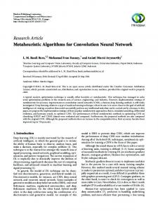
1.3. Problem description This work targets the efficient realization of real-time FIR filters using general-purpose processors. Hence, the considerations are limited to a blockbased audio processing (cp. Sec. A.1). A real-time FIR filtering problem is defined as follows: A continuous audio stream is processed in length-B blocks. B is referred to as the block length. The terms ‘streaming buffer size’ and ‘frame size’ are often used alternatively in audio software development. The sampling rate of the audio stream is fS . The resulting frame rate (processed frames per second) is given by R = fS /B. Unless outlined, a single channel is considered only. Figure 1.1(a) shows the corresponding block diagram. The input signal x(n) consists of consecutive length-B blocks x0 (n), x1 (n), · · · (sub indices denote the individual blocks). It is filtered with finite impulse response h(n) of N filter coefficients. The filtering is processed block by block. When the ith input block xi (n) is fed into the filter, the filtering algorithm computes the corresponding output block yi (n). The computation time is bounded by T = B/fS = 1/R, the duration of one frame. If this time budget is exceeded, the audio stream is interrupted and dropouts are the consequence. Precautions must be taken in order to prevent this. Therefore, a certain safety margin is incorporated and the time budget is not fully exploited. Several subsequent considerations require a clear definition of the audio processing procedure, in particular its events and their timescale. This is given in A.1 in the appendix. The above stated problem considers a single input and single output only (SISO system). The problem can be generalized to multiple inputs and multiple outputs (MIMO system), interconnected by intermediary FIR filters hi→j (n). This is illustrated in figure 1.1(c). All inputs and outputs request and provide blocks of the same length. The admissible time span for computations T is the same as above. Signal processing for auralization often incorporates assemblies of individual filters in serial (figure 1.1(b)) or parallel (figure 1.1(d)). These occur as cascaded filters on a sound path (e.g. directivity, medium attenuation, etc.) or at points of superposition (e.g. the listeners ears, coupling joints between separated spaces). The regarded FIR filters are linear and time-invariant systems (LTI systems). Interaction in virtual environments changes the auralization filters over time. Time-varying FIR filtering has the following meaning in this thesis: at a distinct point in time, a current filter impulse response h0 (n) is replaced with a new filter h1 (n). Strictly speaking, both individual filters are still LTI systems. The exchange h0 (n) → h1 (n) can usually not be accomplished by instantaneous switching of all coefficients within a single sample. This mostly causes audible artifacts. Hence a smooth transition is realized over a number of L output samples. Even within this period, both sets of filter

5

1. Introduction coefficients remain constant. The transition is achieved by crossfading the outputs of both filters. Interaction demands imperceptibly short response times of a virtual reality system. With respect to the filtering, two different types of latency occur: Input-to-output latency is the duration between the events of exciting the filter with a signal and receiving a response at its output. It is adjusted by selecting a reasonably short audio processing block length B. Frequencydomain techniques require the impulse response to be transformed, before it can be used. This transformation consumes time. Moreover, the exchange itself can be bound to specific points in time, which introduces further waiting times. The filter exchange latency describes the delay, when the update of a filter is initiated, until it is exchanged and affects the output of the filter.

1.4. Outline The thesis is organized as follows: Chapter 2 reviews a wide variety of fast convolution methods and assesses their use for real-time filtering. The objective is to identify the most promising base technology for partitioned convolution methods. The chapter’s intention is also to scrutinize FFT-based fast convolution in its status as a standard method. Several divide-and-conquer strategies are examined for their real-time compliance. Chapter 3 introduces the fundamentals of partitioned convolution. Partitions of both operands— signal and filter—are formally defined. Common processing strategies are reviewed. A classification of partitioned convolution techniques is presented. The remaining part of the thesis is dedicated to the study of three of these classes, which are useful for real-time FIR filtering. The subsequent chapter 4 reviews basic and straightforward techniques of real-time filtering using the FFT. These techniques have in common that they do not partition the filter impulse response. The examination of these algorithms aims at the identification of their weaknesses and as proof for the importance of higher-level techniques, which partition the filters as well. Further aspects like filters with multiple inputs and multiple outputs (MIMO filters), assemblies of filters and the implementation of a time-varying filtering are firstly developed for these conceptually simple techniques. Chapter 5 and 6 consider methods with filter partitioning. The state-of-the-art algorithms are presented and their properties are examined in detail. This includes the choice of parameters, their dependencies, the algorithms’ performance and their runtime complexity classes. Towards the end of both chapters the methods are reflected with the advanced aspects, stated above. The benchmark procedure, test system and its performance data is described in depth in chapter 7. Finally, the findings of this thesis are summarized in chapter 8. Some guidelines on the choice of algorithms and parameters are provided. Open scientific questions 6

1.4. Outline

Impulse response x(n)

y(n)

h(n) B

B

Input blocks xi(n)

Output blocks yi(n)

(a) FIR filter (single channel)

x(n)

y(n) h(0)(n)

h(M-1)(n)

(b) Cascade of FIR filters

x(0)(n)

y(0)(n)

h0 0(n)

hM-1

0(n)

x(M-1)(n)

y(N-1)(n)

h0

N-1(n)

hM-1

N-1(n)

(c) FIR filter with multiple inputs and outputs

x(n)

y(n) h(0)(n)

h(M-1)(n) (d) Parallel FIR filters

Figure 1.1.: Types of FIR filters and assemblies

7

1. Introduction are quoted in the outlook. A description of real-time audio processing, comprehensive lists of results and additional mathematical correspondences are found in the appendix.

1.5. Contributions The main contributions of this thesis are: • Review of fast convolution algorithms for real-time filtering and identification of the most suitable methods on general purpose processors. • Classification of partitioned convolution algorithms. The central part of the thesis is dedicated to the examination of the three classes used for real-time filtering: methods with a non-uniform, uniform and no filter partitioning. • Introduction of benchmark-based semi-empirical cost models of the algorithms, allowing to capture and account for specific properties of a target machine. • Examination of uncommon FFT transform sizes (i.e. non powers-of-two) for real-time filtering. • Development of a generalized uniformly-partitioned convolution technique, featuring individual partitions in both operands, input signal and filter. Viable parameters and potential computational benefits are examined. • Considerations on time-varying filtering in conjunction with frequencydomain convolution techniques. Introduction of a computationally efficient formulation of crossfading in the DFT domain. • Considerations on the efficient implementation of MIMO filters with all regarded running convolution techniques. • Considerations on the efficient implementation of sequential and parallel assemblies of frequency-domain filters. • Formal derivation of general timing dependencies in non-uniformly partitioned convolution techniques, also respecting individual sub filter iterations. • Derivation of the runtime complexities of all regarded real-time filtering techniques. Comparison of their computational costs for different filter lengths and latency requirements (block lengths). • Guidelines for the choice of algorithms and selection of parameters for real-time FIR filtering.

8

2. Fast convolution techniques This chapter gives an overview of fast convolution algorithms and their historic evolution. All techniques are reviewed with respect to the previously enumerated objectives and requirements (see section 1.3). The objective of this chapter is to identify the algorithms with the least computational complexity and usability for real-time filtering techniques, which are subject of the subsequent chapters. A fundamental design technique for fast convolution algorithms is to express convolution operations with the concepts and tools of another mathematical field. This facilitates it to apply methods from this field to the original problem. All fast convolution methods have origins in linear algebra, polynomial algebra and number theory or combine techniques from these fields. Matrix diagonalization in linear algebra is a corner stone of transform-based fast convolution algorithms–like FFT-based fast convolution. This class marks the most important class and is reviewed in the most detail in this chapter. Another technique known as interpolation-based convolution has its roots in classical algebra. It makes use of polynomial interpolation to derive simplified equations for discrete convolutions, with fewer terms than the discrete convolution sum. Last but not least did number theory lead to many, often revolutionary, new approaches. Many of these techniques were conceived in the area of fast Fourier transform algorithms and then later applied to convolution methods as well. The central concept thereby have become factorial rings and fields (e.g. calculations modulo integers or polynomials). Many techniques involve the chinese remainder theorem (CRT). In the almost 60 years that passed since the famous paper by Cooley and Tukey [24] had been published in 1965, the fast Fourier transform certainly became very popular and probably the most important tool in digital signal processing. Today, most people associate fast convolution with FFT-based convolution algorithms. And there are several good arguments, why FFTbased convolution is an excellent choice. For instance, the intensive research that has been done on fast algorithms and the availability of very matured high-performance libraries. However, several other approaches to fast convolution have been researched as well. Nowadays, many of these techniques are overshadowed by the enormous success of FFT convolution. FFT-based fast convolution can be thought of as the reference method —not only in this thesis, but also in practice. This chapter scrutinizes this statement and therefore, 9

2. Fast convolution techniques carefully analyzes and compares the algorithmic complexity of very different fast convolution methods. It poses the simple, yet fundamental question: Is FFT-based convolution nowadays the most reasonable technique for real-time FIR filtering on general-purpose processors? The chapter is organized as follows: In the beginning the elementary operations of linear and circular convolution are reconsidered and their relations to the different mathematical areas are shown up. The remaining part of the chapter is dedicated to the review of the three important classes of algorithms, which were enumerated above. Emphasis lies on the most important techniques, in particular FFT-based convolution, but a comprehensive overview of the field is aimed. Most of the methods discussed here, were initially not designed for real-time processing. It is evaluated how they can be adapted to suit this purpose. If possible, the computational complexity is reviewed. The chapter ends with a summary of the methods.

2.1. Discrete convolution Discrete convolution is an operator for two sequences x(n) and h(n) of indefinite lengths. It is defined by the well-known formula [74] y(n) = x(n) ∗ h(n) =

+∞ X

x(k) · h(n − k)

(2.1)

k=−∞

= h(n) ∗ x(n) =

+∞ X

h(k) · x(n − k)

k=−∞

The result of this convolution operation x(n) ∗ h(n) is a sequence y(n), also of indefinite length. In signal processing the sequences are referred to as signals. Discrete convolution is of fundamental importance in system theory. Given a linear and time-invariant system (LTI system), which is fully described by its impulse response h(n), the discrete convolution in Eq. 2.1 defines the

x(n)

y(n) = x(n)

h(n)

h(n) Input signal

LTI system

Output signal

Figure 2.1.: Correspondences between the input signal, the output signal and the filter impulse response of a linear time-invariant system 10

2.2. Linear convolution resulting signal y(n) at the output of the system, when a discrete-time signal x(n) is given into its input (figure 2.1). h(n) is the filter impulse response or short filter. Signals of indefinite length are needed for theoretical analysis. In practical applications on computers, at least the filter h(n) has a definite length (finite impulse response). The domain K of sample values x(n), y(n) and filter coefficients h(n) can be integers (Z), real numbers (R) or complex numbers (C) in floating representation. Two different cases of discrete convolution can be distinguished in Eq. 2.1 • The convolution of two sequences which both have finite lengths. This marks the most general convolution operation on computers. It is the standard operation for offline audio processing, e.g. filtering an audio file with a specific finite impulse response. • The convolution of infinite-length sequence with a finite-length sequence, often called running convolution. A typical application is FIR filtering of a (potentially) infinite stream of audio samples x(n) with a filter impulse response h(n) of a finite length N . This is a typical real-time application, where the output samples y(n) are continuously computed from the input samples x(n) with only a small amount of latency. On computers this is done by means of blocks (or frames) of a specific block length B. The operator in Eq. 2.1 is linear convolution. The relations in Fig. 2.1 are only fulfilled by this operator, making it the desired type of convolution in audio filtering applications. Further discrete convolution operations are known, for instance circular convolution (Sec. 2.3), symmetric convolution or skew-symmetric convolution (Sec. 2.5.6). These operators have favorable mathematical properties. Very often, they are used to realize the desired linear convolution (Sec. 2.3 and Sec. 2.5.6).

2.2. Linear convolution The linear convolution (symbolized by ∗) of a potentially infinite-length sequence x(n) with a length-N filter h(n) = h(0), . . . , h(N − 1) is defined as [73, 74] N −1 X y(n) = x(n) ∗ h(n) = x(n − k) · h(k) (2.2) k=0

The resulting sequence y(n) is a superposition of shifted versions x(n − k) of the original sequence x(n), weighted by the filter coefficients h(k). In case that both sequences x(n) = x(0), . . . , x(M −1) and h(n) = h(0), . . . , h(N −1) have finite lengths M, N ∈ N, the summation in Eq. 2.2 is limited 11

2. Fast convolution techniques to indices k for which both sequences, the shifted x(n − k) and h(k), overlap in at least one element (0 ≤ n−k ≤ M −1 ∧ 0 ≤ k ≤ N −1). Outside these index intervals the values x(n − k) and y(k) are undefined. This yields the definition of linear convolution of two finite-length sequences min{n−M +1,N −1}

X

y(n) = x(n) ∗ h(n) =

x(n − k) · h(k)

(2.3)

k=max{0,n}

From the necessary overlapping of the sequences x(n − k) and h(k) it follows, that the output sequence y(n) has the length M + N − 1.

Matrix-vector product formulation Linear convolution in Eq. 2.2 can be interpreted as a matrix-vector product of the form ~ y = H~x in Eq. 2.4. Burrus and Parks provide detailed explanations on the relations between convolution algorithms and matrix operations in their textbook [21] and give several examples. Let in the following K be a field. K M denotes the M -element vector space over the field K. K M×N is the set of all M ×N matrices defined over K. The sequence x(n) corresponds to a M -element vector ~ x = [x0 · · · xM−1 ]> ∈ K M and y(n) to a vector ~ y = [y0 · · · yM+N−2 ]> ∈ K M +N −1 with M + N − 1 elements accordingly. H ∈ K M +N −1×M is a convolution matrix with M + N − 1 rows and M columns. Its columns contain shifted versions of the sequence h(n), padded by zeros.



h0

  h1   h2   .     .. y0   y1   hN −2     = ..    h .  N −1  yM +N −2   0   0   ..  . 0

12

0

...

h0 h1

... ...

0 .. . 0

h2 .. .

...

h0

hN −2

... .. .

h1 .. .

hN −1 0 .. . 0

... ... .. . 0

hN −3 hN −2 hN −1 ...

0 .. . 0



       0   x  0    x  1 h0   · .    .  .  h1    x M −1 ..  .   hN −3    hN −2  hN −1

(2.4)

2.2. Linear convolution

Polynomial product formulation Linear convolution can also be defined by polynomial products [13]. Sequences are represented by polynomials as algebraic structures. The values x(0), . . . , x(M − 1) and h(0), . . . , h(N − 1) can be interpreted as polynomial coefficients x0 , . . . , xM −1 and h0 , . . . , hN −1 of their two generating polynomials X, H ∈ R[z] with deg(X) = M − 1 and deg(H) = N − 1. R[z] denotes the ring of polynomials defined over a ring or field R and the variable z.1 X=

M −1 X

x(n)z n = x(0) + x(1)z + x(2)z 2 + · · · + x(M −1)z M −1

(2.5)

h(n)z n = h(0) + h(1)z + h(2)z 2 + · · · + h(N −1)z N −1

(2.6)

n=0

H=

N −1 X n=0

Operations on the sequences, like addition, multiplication and shifting, map to operations within polynomial algebra, for instance polynomial addition and multiplication. The linear convolution of the sequences x(n) and h(n) corresponds to the polynomial product y(n) = x(n) ∗ h(n)

= b

Y =X ·H

(2.7)

The resulting polynomial Y ∈ R[z] has the degree deg(Y ) = M +N −2 Y =

M +N X−2

yn z n = y0 + y1 z + y2 z 2 + · · · + yM +N −2 z M +N −2

(2.8)

n=0

with

yk =

k X

xi hk−i

(2.9)

i=0

Its coefficients y0 , . . . , yM +N −2 are defined by a linear convolution in Eq. 2.9 and they correspond to values of the output sequence y(n).

Computational complexity The simplest way to compute a linear convolution is to evaluate the Eq. 2.2 for all output samples. Sometimes, this is cited as direct convolution. In signal processing, this corresponds to filter the input samples with a tapped delay-line (TDL), as shown in Fig. 2.2. In the following the required number of arithmetic operations is derived.

1

In this work z is favored as a polynomial variable, as x is used for sequences and signals.

13

2. Fast convolution techniques

x(n)

h(0)

z-1

z-1

h(1)

h(2)

z-1 h(N-1)

y(n)

Figure 2.2.: Direct-form FIR filter (tapped delay-line) Firstly, the running convolution of an infinite input signal with an N -point filter is considered. As the length of the input signal is quasi-infinite, the computational complexity is assessed by the number of arithmetic operations that are necessary to compute one sample of filtered output. Evaluating Eq. 2.2 for one output value y(n) requires N multiplications and N − 1 additions. The number of arithmetic operations T (N ) per filtered output sample for the direct running linear convolution with a N -tap filter is T (N ) = 2N −1 ∈ O(N )

(2.10)

Secondly, the number of arithmetic operations T (M, N ) for the linear convolution of two sequences with finite lengths M, N is derived from the corresponding N -tap FIR filter (Fig. 2.2). The filtering processing can be split into three phases: • Within the first N −1 steps the accumulators of the filter are getting filled with input samples. Before, they contained zeros. The number of operations in this phase is NP −1 (2i − 1) = N 2 − 2N + 1. i=1

• In the next M−N+1 steps all accumulators contain input samples and Eq. 2.10 applies. The number of operations in this phase is (M −N + 1)(2N − 1). • Now all M input samples have been given into the filter and within the next N −1 the accumulators fill up with zeros again. Here the number of operations is the same as in the first phase. The total number of operations is 2(N 2 − 2N + 1) + (M − N + 1)(2N − 1). Simplifying this expression, the exact number of arithmetic operations for an M×N direct linear convolution is T (M, N ) = 2M N − (M +N −1) ∈ O(M ·N )

14

(2.11)

2.3. Circular convolution Zeros in the accumulators of an FIR filter should not be neglected. A 16×16 linear convolution requires 481 operations. Computing a 16-point running convolution for the same number of 16+16−1 = 31 output samples demands 312 = 961 operations. The time complexity of an N×N direct linear convolution lies within O(N 2 ). Any algorithm that computes the same result in a time complexity lower than O(N 2 ) is considered a fast linear convolution method in the following.

2.3. Circular convolution Linear convolution is aperiodic (or non-cyclic) [73]. Many fast convolution algorithms perform the convolution operation within the domain of some discrete transform (e.g. the DFT), where it can be realized more efficiently. Most of these transforms assume some periodicity of the sequences. The assumption of periodic sequences leads to an adapted formulation of discrete convolution, which is known as cyclic or circular convolution. Let x(n) be a sequence of the finite length N ∈ N. The periodic continuation of x(n) is defined as x e(n) = xhniN , where the indices −∞ < n < ∞ are evaluated modulo the period N . h·iN denotes the residual of the integer n modulo N [68]: hniN = k ⇔ n ≡ k mod N . x e(n) is periodic in N samples. The N -point circular convolution (symbolized by ~) of two length-N sequences x(n) and h(n) is defined as the sum [74] ye(n) = x(n) ~ h(n) =

N −1 X

x e(n − k) · e h(k) =

k=0

N −1 X

xhn − kiN · h(k)

(2.12)

k=0

As the indices of the reversed and shifted sequence xhn − kiN are evaluated modulo N , the output sequence ye(n) is periodic in every N th element as well. Therefore, it is fully determined by N values of ye(n) and has the length N . As the index k is in the range 0 ≤ k < N anyway, the modulo operation can be dropped for the term h(k).

Matrix-vector product formulation The matrix-vector product representation of N -point circular convolution has the form ~ye = C~ x. The length-N sequences x(n), h(n) and ye(n) correspond to N -element vectors ~ x, ~h, ~ye ∈ K N . C = (ci,j ) ∈ K N×N is an N ×N Toeplitz matrix, called circulant matrix (or circular convolution matrix ) [19]. Its elements are ci,j = hhi−jiN (with indices 0 ≤ i, j < N ). C has the special property that each row or column vector is a copy of its neighboring row 15

2. Fast convolution techniques or column vectors, shifted by one element. An example length-5 circular convolution has the form       x0 h0 h2 h1 h0 h2 ye0 ye1  h1 h0 h2 h1 h0  x1        ye2  = h2 h1 h0 h2 h1  · x2  (2.13)       ye3  h0 h2 h1 h0 h2  x3  x4 h1 h0 h2 h1 h0 ye4 Where in a linear convolution matrix the column vectors are zero-padded and shifted versions of the sequence h(n), the circulant matrix contains shifted versions of the N -periodic continuations e h(n). Circulant matrices have an important mathematical property: Their eigenvalues λ0 , . . . , λN−1 are linear combinations of the filter coefficients h(n) with powers of primitive N th roots of unity WN = e−2πi/N ∈ C in the complex number plane [43] N −1 X jk λj = h(k)WN (2.14) k=0

This results in eigenvectors of the form 1 j j 2 j N −1 > ~vj = √ 1, WN , (WN ) , · · · , (WN ) N

(2.15)

Eq. 2.14 corresponds to a N -point DFT of h(n) (cp. Eq. 2.31) and [~v0 , . . . , ~vN−1 ] (Eq. 2.15) defines an eigenvector basis of C. Hence the DFT diagonalizes a circulant matrix, resulting in the cyclic convolution property (CCP). These relations are reviewed in more detail in section 2.5.1.

Polynomial product formulation Circular convolution can be defined using polynomial products as well. The essential difference lies in the algebraic structure, in which the computation is performed. For linear convolution it is computed in the polynomial ring R[z]. In order to obtain circular convolution, the calculation need to be performed in modular arithmetic over the quotient polynomial ring R[z]/(z N − 1) with a polynomial modulus z N − 1 [13]. All polynomials P ∈ R[z]/(z N − 1) have a degree deg(P ) ≤ N . The circular convolution can be computed directly from the linear convolution polynomial Y = X · H ∈ R[z] by evaluating Y modulo z N − 1 [13], realizing the fold-back of overlapping samples into the N -point period. y(n) = x(n) ~ h(n)

16

= b

Y ≡X ·H

mod z N − 1

(2.16)

2.4. Interpolation-based fast convolution This is illustrated in the following example (N = 3): x = 2 −1 3 X = 2 − z + 3z 2 h = 1 2 −1 H = 1 + 2z − z 2 x∗h= 2

3

−1

x~h= 9

0

−1

7

−3

X · H = (2 − z + 3z 2 ) · (1 + 2z − z 2 ) = 2 + 3z − z 2 + 7z 3 − 3z 4 X · H = 2 + 3z − z 2 + 7z 3 − 3z 4 = (7 − 3z) · (z 3 − 1) + (9 − z 2 ) X · H mod z 3 − 1 = 9 − z 2

Example 2.1: Convolutions and corresponding polynomial products

Linear convolution using circular convolution Linear-convolution can be implemented using circular convolution. This makes fast circular convolution algorithms applicable for linear filtering. The relations between both operations are illustrated by the examples in figure 2.3. Let x(n) be a length-M sequence and h(n) a length-N sequence. The result of an M×N linear convolution has the length M + N − 1. The K-point circular convolution equals a M ×N linear convolution, when its period K is sufficiently large, so that the M + N − 1 samples do not overlap in time (avoiding time-aliasing) n o RM+N−1 PK { x(n) } ~K PK { h(n) } = x(n) ∗ h(n) ⇔ (2.17) K ≥M +N −1

(2.18)

For completeness, PK is a padding operator appending zeros until a length K and RM+N−1 is a rectangular window, cutting out the first M+N−1 values of the sequence. Given that condition 2.18 is violated and K < M +N −1, it is not guaranteed that the linear convolution results do not overlap and consequently does the equality Eq. 2.17 not hold anymore.

2.4. Interpolation-based fast convolution The class of methods reviewed first are interpolation-based fast convolution techniques. These are fast algorithms for computing linear convolutions and found on the polynomial product formulation, introduced in section 2.2. Computing the linear convolution x(n) ∗ h(n) translates to the problem of finding the polynomial coefficients y0 , . . . , yM +N −2 of Y (z) (Eq 2.8), as motivated in section 2.2. They can be calculated using direct discrete convolution 17

2. Fast convolution techniques M×N linear convolution x

h

y

M

N

M+N-1

K-point circular convolution (K=M+N-1) ···

x

0

x

0

x

0

···

···

h

0

h

0

h

0

···

···

y

y

y

···

period K

Oversized period (K > M+N-1) ···

y

0

y

Undersized period (K < M+N-1) ···

≠y

Valid results

≠y

0

y

0

···

Time-aliasing ≠y

···

Figure 2.3.: Realizing linear convolution by circular convolution for two example sequences2 (Eq. 2.9), resulting at the runtime complexity of O(M ·N ) (cp. section 2.2). A computational advantage arises from transforming the problem of finding the coefficients yi into an interpolation problem. This allows obtaining formulations (sequences of terms) of linear convolutions that have less arithmetic operations than the naive evaluation. The mathematical framework for interpolation-based convolution is the class of Toom-Cook algorithms. A particular method is the Karatsuba algorithm [54]. It has a runtime complexity O(N log2 3 ) ⊂ O(N 2 ) and is hence considered fast here (cp. section 2.2), although it is asymptotically slower than transform-based approaches in O(N log N ). Unfortunately, interpolation-based techniques become inefficient for longer filters and suit short convolutions only. Their relevance for 2

Correct scaling is neglected

18

2.4. Interpolation-based fast convolution real-time filtering (also with longer filters), stems from their use in accelerating partition convolutions [47] in conjunction with multi-dimensional index mapping (see section 2.6.1). The index mapping techniques are introduced in section 2.6.1 and their application for real-time FIR filtering is reviewed. For a detailed introduction the reader is referred to the textbook by Blahut [13]. Part of this section is the derivation of the exact number of operations for the Karatsuba convolution algorithm, enabling the comparison to alternative methods.

2.4.1. Toom-Cook algorithm The Toom-Cook algorithm was originally conceived by Toom [110] in 1963 as a method for fast integer multiplication. Later in 1966, Cook [23] improved the algorithm. Blahut [13] shows how the technique can be used to implement linear convolution. As motivated above, the problem of linear convolution corresponds to finding the coefficients yk of the product polynomial Y (z) = X(z) · H(z). A fundamental consideration is, that the resulting polynomial Y (z) has deg(Y ) = M + N − 2 and is therefore uniquely determined by M + N − 1 data points. Instead of explicitly multiplying the polynomials X(z) · H(z) using the discrete convolution in Eq. 2.9, the Toom-Cook algorithm evaluates the polynomials X(z) and H(z) for a set of data points αi and then multiplies their values Y (αi ) = X(αi ) · H(αi ). Afterwards the product polynomial Y (z) is constructed using Lagrange interpolation and its coefficients yk are obtained. The algorithm consists of three phases: 1. M + N − 1 distinct supporting points α0 , . . . , αM +N −2 (∀i, j : i 6= j → αi 6= αj ) are chosen. 2. X(αi ) and H(αi ) are evaluated for all supporting points αi and multiplied Y (αi ) = X(αi ) · H(αi ). 3. Y (z) is constructed from the M + N − 1 data points (αi , Y (αi )) using Lagrange interpolation Y (z) =

M +N X−2 n=0

Y (αi )Li (z)

Li (z) =

M +N Y−2 k=0 k6=i

z − αi αk − αi

(2.19)

The interpolation approach results in an alternative formulation of linear convolution, in form of a sequence of terms. These terms group common expressions and remove redundant computations, resulting in less operations than the corresponding direct convolution. Hence, the Toom-Cook method allows deriving fast algorithms for short convolutions. Technically, it computes a factorization H = CGA of the convolution matrix H (Eq. 2.4) [13], 19

2. Fast convolution techniques where G is a diagonal matrix. Given two lengths M, N ∈ N, its parameters of the Toom-Cook algorithm are the M + N − 1 supporting points αi . Ideally, the αi are chosen to be small integers, like 0 and ±1. Then the matrices C and A consist of 0, ±1, making it possible to realize them by a number of pre- and post-additions, but without multiplications. For longer convolutions further supporting points αi have to be chosen. This requires to use larger integers like ±2, ±4, . . . , which show up within the matrices C and A. Unfortunately, this increases the number of multiplications significantly, making the Toom-Cook algorithm reasonable for short convolutions only.

2.4.2. Karatsuba algorithm In 1962 Karatsuba and Ofman [54] published an algorithm for fast multiplication of large numbers with many digits, widely known as the Karatsuba algorithm. For several decades, the algorithm was the de facto fastest known multiplication algorithm for practical problem sizes. This made it a very important tool for the design of hardware multipliers in integrated circuits. Although the original Karatsuba algorithm was originally conceived for fast multiplication of integers, it can also be applied to other algebraic structures, allowing fast polynomial multiplication and as well fast convolution. Blahut [13] presented how the Karatsuba technique, which can be considered a special case of the modified Toom-Cook algorithm, can be applied for fast convolution. Hurchalla [47] showed, that the decomposing scheme of the Karatsuba algorithm conforms with real-time constraints, making the algorithm applicable for low latency filtering. The Karatsuba algorithm is a classic example for a divide-and-conquer strategy. Let x(n) and h(n) be two length-2N sequences. Both sequences are split in half, forming four length-N subsequences x0 (n) = x(0), . . . , x(N − 1)

h0 (n) = h(0), . . . , h(N − 1)

x1 (n) = x(N ), . . . , x(2N − 1)

h1 (n) = h(N ), . . . , h(2N − 1)

The 2N ×2N -linear convolution x(n) ∗ h(n) can be expressed using four N ×N -sub convolutions [47] y0 (n) = x0 (n) ∗ h0 (n)

(2.20)

y1 (n) = x0 (n) ∗ h1 (n) + x1 (n) ∗ h0 (n)

(2.21)

y2 (n) = x1 (n) ∗ h1 (n)

(2.22)

The desired output sequence y(n) of length 4N − 1 is overlap-added from the sequences y0 (n), y1 (n), y2 (n) of length 2N − 1 (as illustrated in Fig. 2.4) y(n) = y0 (n) + y1 (n − N ) + y2 (n − 2N ) 20

(2.23)

2.4. Interpolation-based fast convolution

y0(0

N-1)

y0(N y1(0

2N-2) N-1)

y1(N y2(0

N

2N-2) N-1)

y2(N

2N-2)

Figure 2.4.: Overlap-Add scheme used in the Karatsuba convolution algorithm The Karatsuba algorithm founds on the following equivalence y1 (n) = x0 (n) ∗ h1 (n) + x1 (n) ∗ h0 (n) = [ x0 (n) + x1 (n) ] ∗ [ h0 (n) + h1 (n) ]

(2.24)

− x0 (n) ∗ h0 (n) − x1 (n) ∗ h1 (n) {z } | {z } | =y0 (n)

=y2 (n)

It allows computing the Eq. 2.20-2.22 using three N × N -sub convolutions instead of four, thus saving one N ×N -sub convolution. However, this comes at the expense of 2N further additions ([x0 (n) + x1 (n)], [h0 (n) + h1 (n)]) and 2 × (2N − 1) subtractions (−y0 (n), −y2 (n)). The full potential of this trick is unleashed, when the equivalance is applied recursively. Therefore N = 2k (k ∈ N) is considered to be a power of two. This results in the Karatsuba convolution algorithm, where two length-N sequences (N a power of two) are recursively decomposed and the reduction Eq. 2.24 is applied in every stage. The decomposition ends in trivial 1×1-convolutions y(0) = x(0)·h(0). Computational complexity The runtime complexity of the Karatsuba multiplication algorithm is O(N log2 3 ) [57]. This class also holds for the Karatsuba convolution method. The actual number of operations depends on the implementation. A detailed runtime analysis of the presented algorithm is carried out in the following, revealing the exact number of arithmetic operations, which is used for later comparisons. The trivial case of an 1 × 1-convolution requires a single multiplication (y0 = x0 · h0 ). Let now N = 2k (k ∈ N) be a power of two. Each N × N Karatsuba convolution recursively computes three N/2 × N/2-Karatsuba convolutions (Eq. 2.20, 2.22 and 2.24). Before this step, the intermediate sequences [x0 (n) + x1 (n)], [h0 (n) + h1 (n)] have to be added, requiring 2 × N/2 = N additions. Then, the subtractions in Eq. 2.24 must be performed on 2 × (N − 1) overlapping elements. Finally, the computed intermediate sequence y1 (n) is overlap-added to the (non-overlapping) sequences 21

2. Fast convolution techniques y0 (n) and y2 (n). On close examination, this step consumes N−2 additions, as only N −2 samples actually overlap (see figure 2.4). Alltogether the number of arithmetic operations T (N ) is given by the recurrence N + 4N − 4 (2.25) T (1) = 1, T (N ) = 3T 2 It is helpful to rewrite this expression using the exponent k T 0 (0) = 1,

T 0 (k) = 3T 0 (k − 1) + 4 · 2k − 4

(2.26)

By nesting, this equation can then be transformed into the explicit form T 0 (k) = 7 · 3k − 8 · 2k + 2

(2.27)

Reinserting the definition of N finally yields the total number of arithmetic operations for a N ×N -Karatsuba convolution T (N ) = 7 · 3log2 N − 8N + 2

(2.28)

The runtime complexity class of the algorithm is found by applying the Master theorem [25] to Eq. 2.26. This yields the known [57] runtime complexity class of O(N log2 3 ). Considering that O(N log2 3 ) ⊂ O(N 2 ) the Karatsuba algorithm can be considered a fast convolution algorithm, working entirely in the time-domain. Nevertheless, it is asymptotically slower than O(N log N ) convolution methods (e.g. FFT convolution, cp. Sec. 2.5.2).

2.4.3. Improved Karatsuba convolution A direct 2×2 linear convolution (Eq. 2.3) has the form [ x(0)·h(0), x(0)·h(1) + x(1)·h(0), x(1))·h(1) ]

(2.29)

and requires five arithmetic operations (four multiplies and one addition). In contrast, a 2×2 Karatsuba convolution is slightly more complex [ x(0)·h(0), (x(0) + x(1)) · (h(0) + h(1)) − y0 (0) − y2 (0), x(1)·h(1) ] (2.30) | {z } | {z } =y0 (0)

=y2 (0)

consuming seven operations (three multiplies, two additions and two subtractions). Hence, the Karatsuba ‘trick’ turns out not to be beneficial in every case. As the method decomposes a large convolution into a large number of small 2×2 convolutions, these small convolutions do strongly affect the overall computational complexity of the entire method. Therefore, the author suggests two improvements over the original method [47]: (1) By implementing 2×2 convolutions using direct convolution, the performance can be signifi22

2.4. Interpolation-based fast convolution cantly improved. Table 2.1 shows the number of arithmetic operations for N ×N linear convolutions, including the direct approach and the Karatsuba variants. Apart from interpolation-based approaches, algorithms for very short lengths (N < 10) can be derived by hand, offering some additional savings. Several authors list such short convolution templates—for instance for linear convolution [5, 47] and for circular convolution [73, 13]. Agarwal and Cooley propose a 4 × 4 linear convolution template that requires 20 operations (five multiplies and 15 additions), saving five operations over the direct convolution. The proposed method (2) combines it with the Karatsuba algorithm, so that the Karatsuba decomposition stops at N = 4 and then the template is used. The second approach saves even more operations. In order to constrast the results, table 2.1 also includes the complexity of FFT-based convolution [105] (see Sec. 2.5.2). The data in table 2.1 is visualized in figure 2.5. The numbers consider an implementation using three 2N real-data FFTs [50]. It can be seen that the Karatsuba algorithm is not only fast by means of its asymptotic behaviour, but also in the actual number of operations. This is remarkable in face of that the algorithm works entirely in the time-domain. The improved variant (2) outperforms the direct approach for length N ≥ 4. Interestingly, it also outperforms the FFT-based convolution for lengths N < 128. However, these break-even points might differ in practice. It turned out to be rather challenging to fully develop the Karatsuba technique with respect to exploitation of the available processor capabilities. In contrast high-performance FFT libraries are technically very matured (cp. FFT algorithms in Sec. 2.5.2 and benchmarks in Sec. 7.4).

Arithmetic operations

107 106 105 104 103 102 101 100

4k

2k

1k

51

25

12

64

32

16

8

4

2

1

2

6

8 Operation size N

Direct convolution Improved Karatsuba convolution (2) FFT convolution

Figure 2.5.: Arithmetic complexity of direct N ×N linear convolution, Karatsuba convolution and real-data FFT-based fast convolution (note, that both axis have logarithmic scales)

23

24

1 5 25 113 481 1,985 8,065 32,513 130,561 523,265 2,095,105 8,384,513 33,546,241

1 2 4 8 16 32 64 128 256 512 1,024 2,048 4,096

1 8 33 127 441 1,447 4,593 14,287 43,881 133,687 405,153 1,223,647 3,687,321

Karatsuba convolution (Eq. 2.28) – 5 27 109 387 1,285 4,107 12,829 39,507 120,565 365,787 1,105,549 3,333,027

Karatsuba convolution improv. (1) – – 20 88 324 1,096 3,540 11,128 34,404 105,256 319,860 967,768 2,919,684

Karatsuba convolution improv. (2) 7 26 86 254 686 1,730 4,190 9,830 22,574 50,954 113,534 250,286 547,022

FFT-based convolution (Eq. 2.48)

Table 2.1.: Arithmetic complexity of direct N×N linear convolution, Karatsuba convolution and real-data FFT-based fast convolution

Direct convolution (Eq. 2.11)

Length N


2.5. Transform-based fast convolution

2.4.4. Conclusions The Karatsuba algorithm is an important case of the general class of ToomCook algorithms. It is applicable only for power-of-two sizes N = 2k . However, Toom-Cook algorithms can be derived for many other combinations of lengths M ×N [13]. Hurchalla [47] presents decompositions into three, four and five parts. From the results in table 2.1 it can be concluded, that interpolation-based fast convolution algorithms offer significant computational savings over direct time-domain filtering. Here, the author showed how the Karatsuba technique can be further improved by the use of optimized convolution templates. For short lengths, these methods might also be an alternative to FFT-based convolution—given a well-thought implementation. However, interpolation-based convolution methods can also be seen from a different perspective: they provide efficient schemes to decompose large convolutions into small ones. The fundamental constraint for real-time processing is that these schemes are real-time capable (detailed discussion of these constraints in chapter 6). Hurchulla [47] showed for the Karatsuba algorithm, that even with full nesting, all partial convolution results can be computed in time, making the algorithm real-time compliant. The algorithm does not introduce additional latencies, as all of its nested sub convolutions can be computed in time. However, there is no general ‘zero-latency’ property for the theoretical framework of interpolation-based convolution. Examples of Toom-Cook algorithms can be found [47], where the execution order of the sub convolutions inherits timing dependencies, that result in a large latency.

2.5. Transform-based fast convolution The most important class of fast convolution algorithms, with most frequent use in practice, are transform-based fast convolution methods. They found on two cornerstones: Firstly, a discrete transform, in whose domain the convolution operation is simpler to compute (lower complexity class). Secondly, a fast algorithm to compute the transform in less than O(N 2 ), typically O(N log N ). A method that revolutionized fast convolution is FFT-based fast convolution, published by Stockham [105] in 1966, one year after Cooleys and Tukeys renowned FFT algorithm [24]. Today it is still the most widely known and commonly used fast convolution technique and became widely a synonym for fast convolution. The cyclic convolution property (CCP) of the DFT states, that circular convolution in the time-domain corresponds to the pair-wise multiplication of spectral coefficients in the DFT domain. The mathemat25

2. Fast convolution techniques ical origin of this relation can be traced back to matrix diagonalization in linear algebra. By computing DFTs using FFT algorithms, a fast circular convolution method in O(N log N ) ⊂ O(N 2 ) is obtained. With appropriate zero-padding, the technique can be used to realize fast linear convolution as well. The DFT demands complex-valued arithmetic, which especially on those early day computers was rather expensive to realize. This motivated research in real-valued transforms. A promising alternative to the DFT was the discrete Hartley transform (DHT). Other considered candidates are discrete trigonometric transforms (DTTs), including the variety of discrete sine transforms (DSTs) and discrete cosine transforms (DCTs). Fast algorithms exists for all of the cited transforms. Unfortunately, none of them holds the strict CCP and thus, spectral convolutions become more than just a pairwise product of spectral coefficients. For discrete trigonometric transforms (DTTs) in particular, such a convolution multiplication property (CMP) only exists for special convolution operators. Yet the real-valued transform techniques are worth the consideration as an alternative to FFT-based convolution, in particular when hardware transformers are available or the input data is already within the domain of the transforms. All of the above mentioned transforms are defined over trigonometric functions and hence rely on floating-point arithmetic. Interestingly, integer-based transforms with similar properties as the DFT exist. A starting point was the extension of the DFT to finite fields by Pollard [75] in the 1970s. Instead of using the complex number plane, a transform of similar structure to that of the DFT can be defined in modulo arithmetic over integers. In successive years a variety of methods has been proposed, which constitutes the class of number theoretic transforms (NTTs). These transforms have the CCP. The existence of fast NTTs algorithms allows realizing a numerically exact fast convolution without round-off errors. Especially for the design of hardware convolution units, they turned out to be very beneficial, reducing the complexity of circuits. However, number theoretic transform (NTT)based convolution never reached the same level of popularity as FFT-based convolution. This section reviews transform-based convolution techniques in the face of real-time filtering and identifies the computationally most efficient one. Aspects of hardware design are not considered here. The focus lies on software implementations on current general purpose processors. A main part of the section is dedicated to the review of FFT-based convolution. Improvements to the original FFT-based convolution technique are discussed. The computational complexity of the FFT convolution techniques is carefully examined. Afterwards, real-valued transforms and NTTs are discussed as alternative techniques. It is outlined how convolution can be realized in the domains of 26

2.5. Transform-based fast convolution these transforms. The complexity is analyzed and is compared to the one of the FFT-based approach, determining if they are actual alternatives.

2.5.1. Discrete Fourier Transform The length-N discrete Fourier transform (DFT) [73, 21, 74] transforms a sequence x(n) = x(0), . . . , x(N − 1) into a N -point DFT spectrum X(k) = X(0), . . . , X(N−1) (Eq. 2.31). x(n) can be recovered from the DFT spectrum X(k) using an inverse DFT (Eq. 2.32). DF T

x(n) c

s X(k) =

N −1 X

nk

x(n) e −2πi N

n=0

=

N −1 X

nk x(n) WN

(2.31)

n=0

DF T −1

X(k)

s

N −1 N −1 X nk 1 X −nk c x(n) = 1 X(k) e 2πi N = X(k) WN

N

N

k=0

(2.32)

k=0

−nk nk and WN of the DFT and IDFT are powers of the N th The kernels WN primitive root of unity W −2πi/N in the complex number plane C. In general, the input and output values are complex numbers x(n), X(k) ∈ C. Eq. 2.31 and 2.32 can also be interpreted as matrix-vector products of the form −1 ~ ~ = FN ~x (DFT) and ~ ~ ∈ CN and DFT X x = FN X (IDFT), with vectors ~ x, X −1 ∈ CN ×N matrices FN , FN 1 −jk jk −1 F N = WN FN = WN (2.33) N 0≤j,k

ye(n) = x(n) ~ h(n) = 14 3 6 2

~ye = C · ~ x    1 −1 3 2 2  2 1 −1 3  −1   =  3 2 1 −1  ·  3 −1 3 2 1 1 {z } |

   

=C

> = 14 3 6 2

DFT 4

 1 1 1 1 1 −i −1 i  F4 =  1 −1 1 −1 1 i −1 −i

   

  1 1 1 1 1 1 i −1 −i   =  4 1 −1 1 −1  1 −i −1 i

DFT 4−1

F4−1

X(k) = DF T 4 { x(n) } = 5 −1+2i 5 −1−2i

~ = F4 · ~ X x > = 5 −1+2i 5 −1−2i

H(k) = DFT 4 { h(n) } = 5 −2−3i 3 −2+3i

F4 · C · F4−1 =  5 0 0 0  0 −2−3i 0 0   0 0 3 0 0 0 0 −2+3i

   

Y (k) = X(k) · H(k) = 25 8−i 15 8+i

~ = diag(5, −2−3i, 3, −2+3i) · X ~ Y > = 25 8−i 15 8+i

ye(k) = DF T 4−1 { Y (k) } = 14 3 6 2

~ye = F −1 · Y ~ 4 > = 14 3 6 2

Example 2.2: DFT-based length-4 circular convolution and corresponding matrix-vector representations (C circulant matrix, F4 4-point DFT matrix, F4−1 4-point inverse DFT matrix)

29

2. Fast convolution techniques Zero-padding to length K Complex-valued multiplication x(n)

K

K-point FFT K-point IFFT

h(n)

K

M+N-1

y(n)

K-point FFT

Extraction of the first M+N-1 values

Figure 2.6.: Fast linear convolution realized by circular convolution in the DFT domain, implemented using fast Fourier transforms (FFTs), as proposed by Stockham [105] FFT-based fast convolution Let x(n) be a length-M and h(n) a length-N sequence. The M ×N linear convolution x(n) ∗ h(n) in O(K log K) can be computed in O(K log K), by implementing Eq. 2.34 using K-point FFTs. The transform size K must satisfy K ≥ M + N − 1 (Cond. 2.18), otherwise the linear convolution is corrupted (see section 2.5.1). Figure 2.6 illustrates this well-known method, which was proposed by Stockham [105]. Initially both sequences are padded to length K, expressed by a padding operator PK and transformed using K-point forward FFTs. The resulting K-point DFT spectra X(k) and H(k) are pairwisely multiplied using K complex-valued multiplications. These are referred to as ‘spectral convolutions’. The result is transformed back into the time-domain using a K-point inverse fast Fourier transform (IFFT). Given that K > M +N −1 the first M + N − 1 samples are selected, represented by the trim operator RM+N−1 . The runtime complexity is a function of the transform size K, determined by the sequence length M, N , of the following general form TCONV-FFT (K) := 2 TFFT (K) + TCMUL (K) + TIFFT (K) with

K ≥M +N −1

(2.37) (2.38)

The terms TFFT (K), TIFFT (K) and TCMUL (K) express the computational complexity (number of arithmetic operations, central processing unit (CPU) cycles or runtimes). The general formula in Eq. 2.37 will be refined in later sections and chapters. Possible points for optimization can already be identified here: transformations and spectral convolutions. The choice of the transform size K is crucial for the performance of the algorithm. This aspect is reviewed in detail in section 4.1.4. If the filter h(n) remains unchanged, the spectrum H(k) can be reused for multiple input signals and one forward 30

2.5. Transform-based fast convolution FFT can be dropped from Eq. 2.37. By time-reversing one sequence the method can be used to compute fast correlations [105]. General DFT spectra consist of complex-valued coefficients. Real-valued input data introduces symmetries to the DFT spectra, so that effectively only half of the coefficients need to be stored and processed. The details are examined later, at the end of this section. The inevitable zero-padding of the input sequences is unfortunately carried into the computation of the FFTs. Transform algorithms process many ineffective zeros. Techniques to save operations from these circumstances are reviewed in section 2.5.4 on partial transforms. A further simplification arises for even or odd sequences, which have purely real respectively imaginary DFT coefficients. The resulting arithmetic simplifications are examined in section 2.5.3. Computing the Fast Fourier Transform This section gives a brief overview on the current state of the art in computing the fast Fourier transform. The focus lies on the algorithmic design principles and in particular on the decomposition techniques for obtaining divide-and-conquer algorithms for the fast computation of the DFT. Only the most important milestones with respect to fast convolution are outlined here, serving as the basis for the discussion of enhancements in FFT-based fast convolution techniques. These do not regard the FFT as a black box, but try to exploit certain properties of the transform and the transform algorithms. A compact overview on the state of the art in computing the FFT can be found in [29]. For a more comprehensive introduction, including the mathematical backgrounds, the author recommends the textbooks by Nussbaumer [73] and Burrus and Parks [21]. History of the FFT The FFT is presumably one of the most intensively researched algorithms in history and numerous papers have been published about it [115]. In the year 2000 issue of ‘computing in science and engineering’ the FFT was credited one of the ‘top ten algorithms of the century’ [26] with the ‘greatest influence on the development and practice of science and engineering in the 20th century’. In 1965 John W. Tukey and James W. Cooley published a groundbreaking paper on the fast computation of discrete trigonometric series [24]. This publication is widely considered as ‘the original fast Fourier transform’. In their paper they derive the famous radix-2 DIT FFT algorithm as an example, which lead to the widespread belief, that the Cooley-Tukey FFT is only suitable to compute power-of-two FFTs. But it is not. The scientific impact of Cooley’s and Tukey’s algorithm is reasoned by the fact, that they 31

2. Fast convolution techniques developed an algorithm for any FFT length N which is not a prime number. The essential contribution of their paper is the composition of a large DFT into several DFTs of smaller sizes by utilizing an index-mapping technique called common-factor map (CFM). The use of this mapping requires intermediate multiplication by complex constants, called twiddle factors [40], which account for the most computation. A thorough study in the mid 1980s [45] revealed that the German mathematician Carl Friedrich Gauss can be considered the first inventor of the FFT. Gauss developed an algorithm which is mathematically equivalent to the Cooley-Tukey twiddle-factor FFT. The reader is encouraged to read the interesting paper by Heideman, Johnson and Burrus [45], from which some key findings are cited in the following. Gauss who used his algorithm for computing the trajectories of asteroids, did not publish the algorithm in his lifetime. It was rediscovered posthumously from his collected publications. His invention cannot be dated accurately, but very likely it even predates Fourier’s publications on harmonic analysis in 1807 [45]—the origin of the discrete Fourier transform. In the following 150 years several fast algorithms for discrete trigonometric series have been invented, published and used [45] (first for some fixed length 4, 8, 12, 16, 32, later for multiples of powers 2n k, 3n k). However, none of these results were as general as Gauss’ and Cooley’s and Tukey’s results and could be applied for arbitrary composite transform sizes. A milestone before the Cooley-Tukey FFT was the GoodThomas prime-factor algorithm (PFA) [42, 109], published 1958. It allows the efficient computation of length-N DFTs, when N is assembled from coprime factors (e.g. 15 = 3 · 5). Thereby it makes use of an index mapping called prime-factor map (PFM). It cannot be used for factorizations with common factors (e.g. 20 = 2 · 10 where gcd(2, 10) = 2). The prime-factor algorithm does not require multiplications with intermediate twiddle factors, like for the Cooley-Tukey FFT, but unfortunately it does involve the computation of many prime-size DFTs. Today the PFA still serves as a decomposition principle for computing FFT of arbitrary sizes, that are not primes. Further remarkable achievements were the publication by Rader [77] in 1968 and Bluestein [14] in 1970, who showed how DFTs can be computed by circular convolutions. In particular Raders method reexpresses an N -point primesize DFT as an N−1-point circular convolution, with the help of the discrete logarithm [77]. Eventually, this circular convolution is then realized using regular FFT techniques again, which do not involve prime-size transforms anymore. This approach paved the way to fast O(N log N ) algorithms for computing prime-size FFTs. Yet it should be remarked, that these primesize FFTs compute several magnitudes slower than power-of-two FFTs (see benchmarks in chapter 7). Winograd [127] suggested to use Rader’s primesize FFTs concept in conjunction with the PFA, where it is used to compute prime-size FFT efficiently. This algorithm, known as the Winograd Fourier 32

2.5. Transform-based fast convolution transform algorithm (WFTA), also provides a lower bound for the number of multiplications for an FFT. Unfortunately, the algorithm comes along with an increased number of additions, making other techniques faster in practice. Based on the original Cooley-Tukey CFM mapping, several other radices (radix-4, radix-8, etc.) have been developed and it has been shown that these transforms can save further operations over the classical radix-2 FFT [10]. A major step forward in reducing the arithmetic complexity of the FFT happened with the invention of the split-radix FFT. Originally conceived by Yavne in 1968 [129] it remained largely unnoticed for many years [115]. Split-radix FFTs decompose an N -point DFT into two N/4-point DFTs and one N/2-point DFT. Duhamel and Holland [27] reinventend this decomposition concept in 1984 and popularized it. A split-radix FFT can be computed for any transform length N that is dividable by 4. Until today split-radix FFTs achieve the lowest operation counts for power-of-two sizes N [115, 27, 50]. At the time of writing, the most recent and advanced FFT algorithms for complex and real data for power-of-two sizes were the split-radix algorithms by Johnson and Frigo [50]. Not only these algorithms are part of the FFTW library [34], but also do the authors provide exact formulas for the number of arithmetic operations. In this thesis, these two algorithms are mostly used for theoretical comparisons. Besides this line of developments aiming for general FFT transforms, a scientific topic of great interest became specialized transforms for real-valued input data, known as real-data FFTs. By exploiting the complex-conjugate symmetry in DFT spectra of real-valued input data, these algorithms compute an N -point real-data FFT in approximately 50-60% of the runtime of a complex-valued N -point transform. The application of the FFT for digital filtering was proposed by Stockham in 1966, shortly after the reinvention of the FFT by Cooley and Tukey. Stockham [105] showed how the FFT could be used for fast convolution and fast correlation. Realizing fast linear convolution using fast circular convolution in the DFT domain, involved zero-padding of the input sequences. When computing running convolutions using Overlap-Save (OLS), a subset of the IDFT output values is needed. For these cases partial FFT transforms have been proposed. These concepts will be reviewed in detail in section 2.5.4. The computational savings by partial transforms for digital filtering turn out to be little. Many of the algorithmic concepts derived for FFTs apply to other discrete transforms as well [29]. This includes the discrete Hartley transform, the family of discrete trigonometric transforms, as well as the NTTs . For all of these transforms fast O(N log N ) algorithms exist.

33

2. Fast convolution techniques Computing FFTs today Nowadays, FFTs are mostly computed using matured high performance libraries, like FFTW [34], Intel’s Math Kernel Library (MKL) or Performance Primitives (IPP ), AMD’s Math Core Library (ACML) or Apples vDSP library. These libraries can be considered as collections of FFT building blocks. FFTW is thereby of particular scientific interest, as it is open-source software and its internal design is well-documented [36]. Furthermore, it computed the most complete set of discrete transforms of all mentioned libraries. The libary consists of a set of small-size fast Fourier transform (FFT) assembly language templates, called codelets (e.g. a length-32 real-data DFT). These templates can be specific for machines or instruction sets. On top of this, the libray holds various decomposition schemes (e.g. a radix-2 Cooley-Tukey decomposition). Before an FFT can be computed, the user has to plan the transform, providing the library the transform properties (real vs. complex, dimensions, data alignment, etc.). Then FFTW figures out the most performant decomposition of the desired transform maximizing the execution speed. This process can be guided and adjusted for other attributes (e.g. numerical stability). The library has been extensively benchmarked by the author for this thesis. The results are presented in chapter 7. Real-valued input data In audio processing, the input data and filter coefficients are usually realvalued. The N -point DFT (Eq. 2.31) is a complex-valued transform DFT (N) : CN → CN , mapping N complex input values x(n) ∈ C to N complex DFT coefficients X(k) ∈ C. For the case that all N input values are real x(n) ∈ R, the corresponding DFT spectrum X = DFT (N ) { x(n) } holds the Hermitian symmetry [74] X(k) = X(N −k) (2.39) Hence, the full N -point DFT spectrum can be reconstructed from C complexconjugate symmetric (CCS) DFT coefficients, where (N + 1, N even N +1 C= = N2 +1 (2.40) 2 , N odd 2 Real-data FFT algorithms exploit these symmetries and compute roughly twice as fast as their complex-valued counterparts. An N -point real-tocomplex (R2C) FFT maps N real-valued samples to C DFT coefficients (Eq. 2.40). An N -point complex-to-real (C2R) IFFT is the corresponding inverse transform.

34


N even

N odd

X(0)

0

X(1)

X(1)

X(0)

0

X(1)

X(1)

X(N/2-1)

X(N/2-1)

X(N/2)

0

X([N-1]/2) X([N-1]/2)

Figure 2.7.: Memory layout of complex-conjugate symmetric N -point real-data DFT spectra P −1 n·0 (DC Since all x(n) ∈ R, the first DFT coefficient X(0) = N n=0 x(n)WN offset) is always real-valued, too. In case the transform size N is an even number, the central DFT coefficient X(N/2) is purely real valued as well. Figure 2.7 shows the commonly used interleaved memory layout for complexconjugate symmetric (CCS) DFT spectra. The zero imaginary parts can be dropped, resulting in the most compact representation, which is known as packed format [1]. With respect to symmetry, a real-data DFT effectively maps N floating point elements to N floating point elements (bijection). In the following the number of arithmetic operations required for spectra convolution of two real-valued DFT spectra is analyzed. A coarse estimate arises from the observation that only C complex-conjugate symmetric coefficients have to be multiplied, requiring 6C operations   6 N2 + 1 = 3N + 6 N even TCMUL-CCS (N ) = 6C = (2.41)  6 N +1 = 3N + 3, N odd 2 Looking into detail, all purely real-valued pairs of coefficients X(0)·H(0) and X(N/2) · H(N/2) for even N , can be multiplied using a single arithmetic operation, saving a couple of instructions   N even 6 N2 − 1 + 2 = 3N − 4 TCMUL-CCS (N ) = (2.42)  6 N +1 − 1 + 1 = 3N − 2, N odd 2 This precise statement complicates the theoretical analysis of algorithms, as conducted in the preceding chapters. The following simplification is often preferred N TCMUL-CCS (N ) ≈ TCMUL = 3N (2.43) 2 For reasonably large N this is a close estimate. For N = 128 the relative error is 1.05% (384/380) and N = 1024 it is 0.13% (3072/3068).

35


2.5.3. Symmetric filters Sequences with an even or odd symmetry have DFT spectra which are either entirely real-valued or purely imaginary (Eq. 2.44 and 2.45) [74]. The general complex-valued the spectral convolutions simplify in these case, which allows saving operations. Input signals in audio processing are usually real-valued, but they do usually not inhere these symmetries. Their DFT coefficients are therefore complex-conjugate symmetric, but in general complex-valued. Neither the real nor the imaginary parts do completely vanish. In contrast, some types of filters hold the contemplated symmetries and allow further arithmetic simplifications. For symmetric respectively antisymmetric realvalued length-N impulse responses h(n) ∈ R the following relations hold DF T (N)

h(n) = h(N − n) even

c

s

H(k) real

(Im{H(k)} = 0)

(2.44)

H(k) imag. (Re{H(k)} = 0)

(2.45)

DF T (N)

h(n) = −h(N − n) odd

c

s

A class of filters that satisfies these properties are causal generalized linear phase FIR filters [74]. In acoustic virtual reality they are for instance used in the form of linear-phase wall-impedance filters in room acoustic simulation methods or as headphone equalization filters. For the case that the impulse response is real and even, the spectral convolutions can be realized using just two multiplies (Eq. 2.46) instead of six operations per DFT coefficient. Accordingly, for an odd symmetry an additional change of sign is necessary (Eq. 2.47). (a + bi)c = ac + bci (a + bi)di = −bd + adi

(2 multiplies)

(2.46)

(2 multiplies, 1 negation)

(2.47)

Exploiting these symmetries in practice is hindered by the following constraints: the necessary zero padding (cp. Sec. 2.5.1) must be realized so that the symmetry properties (Eq. 2.44 or 2.45) are maintained. Otherwise, complex-valued DFT coefficients appear in H(k). This can be assured by zero-padding on both sides and claiming that h(0) = 0. However, the savings in the arithmetic allow marginal speedups only, as the spectral convolutions demand little computation only (see figure 4.4). In partitioned convolution techniques the FFTs play a less dominant role and more computation falls back to spectral convolutions. Here however, the symmetry properties are sacrifized by the partitioning of the impulse response. Symmetries of a complete (unpartitioned) filter (symmetric or antisymmetric) do not translate into symmetries in the subfilters, thus making the simplifications unapplicable. In conclusion, only little computational savings can be expected for the case of symmetric filters. 36

2.5. Transform-based fast convolution Computational complexity This thesis considers several fast convolution methods which are based on the FFT. As this chapter aims the comparison of general fast convolution concepts, one representative FFT-based convolution technique had to be selected. Chosen was the basic method in Fig. 2.6, implemented with real-valued FFT transforms and making use of the previously discussed symmetries. With these considerations, the computational costs for FFT-based convolution in Eq. 2.37 are refined to the following function TCONV-FFT (K) := 2TFFT-R2C (K) + TCMUL-CCS (K) + TIFFT-C2R (K)

(2.48)

As before, the transform size K must hold condition 2.37 in order to achieve linear convolution, as it is desired. An N ×N linear convolution (N = 2k ) is computed with a transform size of 2N points. FFTs are computed using the real-data split-radix FFT by Johnson and Frigo [50]. It is assumed that the inverse FFT has the same number of operations. Spectral convolutions account for the number of operations in Eq. 2.42. Table 2.2 lists the number of arithmetic operations for the basic operations (FFTs, spectral multiplications) and the entire algorithm. The data is completed by the costs of a direct linear convolution in the time-domain (Eq. 2.3). It can be seen, that the major computational load falls back on the FFTs, while spectral convo-

Length N

Real-data split-radix FFT, IFFT (Eq. in [50])

Complex multiplies (Eq. 2.42)

FFT-based convolution (Eq. 2.48)

Direct convolution (Eq. 2.11)

1 2 4 8 16 32 64 128 256 512 1,024 2,048 4,096

2 6 22 70 198 514 1,270 3,022 7,014 15,962 35,798 79,334 174,150

1 8 20 44 92 188 380 764 1,532 3,068 6,140 12,284 24,572

7 26 86 254 686 1,730 4,190 9,830 22,574 50,954 113,534 250,286 547,022

1 5 25 113 481 1,985 8,065 32,513 130,561 523,265 2,095,105 8,384,513 33,546,241

Table 2.2.: Arithmetic complexity of N ×N linear convolutions implemented using the FFT (Fig. 2.6) and by direct convolution (Eq. 2.3) 37

2. Fast convolution techniques lutions make up for a minor part only. Until the length N = 16 the direct convolution requires less operations. Then the FFT approach takes the lead. Vast savings due to the lower complexity class O(N log N ) ⊂ O(N 2 ) become apparent for larger N . For N = 4096 the FFT approach is > 60 times more efficient than the direct convolution. The improved Karatsuba convolution (variant 2) (section 2.4.2) outperforms the FFT-convolution for small sizes N < 128. But also for sufficiently large N , the FFT method clearly wins (O(N log N ) ⊂ O(N log2 3 )). For N = 4096 the Karatsuba technique (2) is ≈ 5.3 times less efficient.

2.5.4. Partial DFTs The majority of FFT algorithms is designed and optimized to compute complete transforms, including all input and output points. Particularly in convolution algorithms, it often occurs that only a subset of the input or output points of a transform are of interest. Input samples and filters are often zero-padded to match the transform size. By considering only the nonzero elements in the FFT algorithm, arithmetic operations could be saved over computing a complete transform. Computing a K-point DFT from only L < K nonzero input samples, is known as a partial input DFT. In practice, an FFT is often computed of blocks of samples from which half are zero L = N/2. These cases are illustrated in Fig. 2.8. They occur frequently in techniques for computing running convolutions. A detailed study of these method is given in chapter 4. This is typically the case for the input data in Overlap-Add (OLA) running convolutions and the transformation of subfilters in partitioned convolution methods. It is referred to as a half-input FFT in the following. The case when only a subset of output points from an inverse FFT is needed, is referred to as a partial output IDFT. This case often occurs in OLS running convolution algorithms, where part of the IDFT results are discarded. The case when one half of an IFFT is desired is called a half-output IDFT in this work. Specialized algorithms for fast partial transforms could thereby turn out to be beneficial for speeding up the convolution.

N

x0(n) N/2

(a)

N

N

x1(n)

x0(n)

N/2

N/2

(b)

0

0

N/2

N/2

x1(n) N/2

(c)

Figure 2.8.: Block decomposition of a signal into two halves

38

2.5. Transform-based fast convolution In this section, techniques for partial transforms are reviewed and discussed. The examination is based on partial FFTs, for which most concepts have been developed. The techniques reviewed here can be applied to several other transforms as well (e.g. NTTs), which share common mathematical properties (e.g. decomposition) and algorithmic origins (e.g. divide-andconquer designs). Particular attention is paid to the benefit of these rather specialized algorithms in today’s times of highly optimized, general purpose FFT libraries. Goertzel algorithm The Goertzel algorithm [41, 21, 13, 74] is a method allowing to compute individual coefficients of a DFT or IDFT, independent of each other. The algorithm is more efficient than the direct computation of a DFT coefficient X(k) in Eq. 2.31. The starting point is to substitute part of the Fourier kernel j WN in Eq. 2.31 by the variable z. The summation of a single DFT coefficient X(k) can be understood as evaluating the polynomial p(z) = x(0)z 0 + · · · + k ) = X(k). The principle behind the x(N − 1)z N −1 in the point p(z = WN Goertzel algorithm is turning this computation into a recursive digital filter (see Fig. 2.9). Firstly, Horners rule [93] is applied to evaluate p(z) efficiently. The resulting sequence of nested terms can be rewritten in form of a linear difference equation, defining a recursive filter. The samples x(n) are given into the filter. After N filtering steps the output value y(n) equals the desired DFT coefficient. The straightforward derivation of the algorithm leads to the so-called first order Goertzel algorithm, which involves a single feedback path with a complex multiplication. This algorithm can be modified into a second-order Goertzel algorithm [74], as shown in figure 2.9. This structure is computationally more efficient by saving complex multiplications for real-valued input samples x(n). −k The remaining complex multiplication with WN in the feed-forward branch only needs to be evaluated in the final N th step [74] (marked gray). The author analyzed the example code of second-order Goertzel algorithm in [21] and found the number of operations for computing a single coefficient X(k) of an N -point DFT to be 6N + 8. Consequently, the Goertzel algorithm’s runtime to compute a complete N -point DFT is in O(N 2 ). This implies that the algorithm is only beneficial, when a very small number L N of DFT coefficients shall be computed. The break-even point, for that a complete N -point FFT is cheaper to compute than an L-point Goertzel algorithm can be roughly evaluated with N/ log2 N [74]. The author compared the second-order Goertzel algorithm’s number of operations for real-valued inputs with a more recent real-data split-radix FFT algorithm [50]. Given a practical transform size of N = 128, the Goertzel 39

2. Fast convolution techniques algorithm is only more efficient when computing a single DFT coefficient (L = 1). Even for larger transforms N = 4096 the break-even point is L ≤ 3. This renders the Goertzel algorithm unfeasible for partial transforms in fast convolution algorithms. Pruned FFTs A more efficient strategy for computing partial DFTs can be directly derived from fast Fourier transform algorithms. Markel [65] presented a technique based on the radix-2 decimation-in-frequency Cooley-Tukey FFT [24] for computing partial FFT, either with partial input data or partial output data. The computation on a FFT can be visualized using a flow graph (e.g. figure 2.10 and 2.11). The intermediate FFT computations are often referred to as butterflies [21], due to their crossed calculation paths. Computational savings are for a partial DFT achieved by pruning the flow graph and removing the computations of undesired values and computations that involve ineffective zeros. Further savings arise from the fact, that with pruning, several butterflies in an FFT flowgraph only need to be evaluated half, if one of the two input values is zero. For L N some butterflies in the flowgraph may be completely dropped, if both of its inputs are zero. Skinner [96] applied pruning to the DIT-FFT and improved Markel’s method further, by reducing the number of twiddle factor multiplications in the first stages. Sreevinas and Rao [103] described a combined FFT algorithm with both, input and output pruning. The computational savings of a Markel pruned FFT over a complete FFT are approximately n(l + 2(1 − 2−(n−l) ))−1 − 1 [65], where N = 2n , L = 2l . The computational savings of both pruning concepts are analyzed in [100] in detail. Markel’s pruning [65] is illustrated in figure 2.10 in the example of an 8-point half-input FFT. The second half of input samples is considered to be zero

y(n)

x(n)

WN-k

x(n)

y(n)

2cos

2 k N

z-1

WN-k

-1

z

-1

z-1

Figure 2.9.: First- and second-order Goertzel algorithms for computing individual DFT coefficients [74] 40

2.5. Transform-based fast convolution here x(n ≥ N/2) = 0, L = N/2. Savings in the algorithm are achieved in the first butterfly, which only needs to be evaluated half. The remaining flowgraph remains identical. The computational savings over a complete FFT are 8 additions and 4 multiplications and thereby little. All 12 twiddle factor multiplications remain. Figure 2.11 shows the corresponding Skinner DIT-FFT. It saves as well 8 additions and 4 multiplications, but it requires only 8 twiddle factor multiplications. Both examples illustrate, that the computational savings for both algorithms are little. Further studies can be found in [100], where pruning is compared to modern split-radix FFTs. The authors conclude, that reasonable savings can only be achieved if a small number of points L N is considered. For L ≥ N/2 they advise to compute full transforms instead. A disadvantage of the pruning concepts is that they are essentially low-level techniques which modify an FFT algorithm. This does not go well along with current trends in FFT implementations and their extensive optimization. All present major FFT libraries (FFTW, IPP, MKL, ACML) are designed to compute full transforms and do not support pruning. Typically, a highly-optimized full transform computed with such a library will outperform a pruned FFT, that is derived by hand. The authors of FFTW [35] argue that the moderate savings by pruning are disproportionate to the effort of generating high-performance pruned implementations. They suggest not to consider pruning unless 1% or even less of the input/output values is needed [35]. A recent study [33] compares complete FFT to pruned FFT. Here, vectorized high-performance FFTs were specifically created using code generation techniques. This includes half-input and half-output pruned FFTs. The results of their practical benchmarks support the prior findings, that the savings for half-input or half-output FFT are little. Transform decompositions An elegant, systematic and even computationally more efficient alternative to pruning techniques are transform decompositions [100]. Based on a CooleyTukey decimation-in-frequency (DIF) decomposition [24], a large DFT is divided into several smaller DFTs using two-dimensional index mapping. The partial input data needs to be multiplied with twiddle factors. Then, regular complex FFTs are computed of these intermediate signals. The coefficients of the complete DFT are obtained by selection. In the following, the method by Sorensen and Burrus [100] is outlined.

41


x(0)

X(0) 0 WN

x(1)

-1 0 WN

x(2)

X(2)

-1 2 WN

x(3)

-1

0 WN

-1

W N0

x(4)

W N1

0 WN

-1

-1 W N2

x(6)

0 WN

-1

2 WN

-1

-1

X(5)

X(3)

-1 W N3

x(7)

X(6)

X(1)

-1

x(5)

X(4)

0 WN

-1

X(7)

Figure 2.10.: Flow graph of an 8-point radix-2 decimation-in-frequency (DIF) input pruned3 FFT [65]

x(0)

x(4)

X(0) 0 WN

0 WN

x(2)

x(6)

X(1)

-1

2 WN

-1

W N0 -1 0 WN

W N1 -1

-1 0 WN

x(3)

x(7)

X(3)

-1

x(1)

x(5)

X(2)

-1 0 WN

W N2 -1

0 WN

2 WN

-1

-1 W N3

-1

-1

X(4)

X(5)

X(6)

X(7)

Figure 2.11.: Flow graph of an 8-point radix-2 decimation-in-time (DIT) input pruned3 FFT [96]

3

The second half of the input is zero x(n ≥ 4) = 0

42

2.5. Transform-based fast convolution Transform decomposition requires a transform size N that can be factored into N = P · Q (P, Q ∈ N). Then an index mapping of the following form can be defined n = P · n1 + n2

n1 ∈ {0, . . . , Q − 1},

n2 ∈ {0, . . . , P − 1}

(2.49)

k = k1 + Q · k2

k1 ∈ {0, . . . , Q − 1},

k2 ∈ {0, . . . , P − 1}

(2.50)

Let x(n) now be the length-N sequence of which an N -point DFT X(k) shall be computed. Substituting the indices n, k in the definition of the DFT (Eq. 2.31) by the mapping in Eq. 2.50 yields [100] X(k1 + Qk2 ) =

P −1 Q−1 X X

(P n1 +n2 )(k1 +Qk2 )

x(P n1 + n2 )WN

(2.51)

n2 =0 n1 =0

=

P −1 X n2 =0

"

Q−1

X

# x(P n1 +

(P n +n )k n2 )WN 1 2 1

WPn2 k2

(2.52)

n1 =0

The outer sum in Eq. 2.52 can be read as an P -point DFT Xk1 (k2 ) =

P −1 X

xk1 (n2 )WPn2 k2

(2.53)

n2 =0

of a signal xk1 (n2 ), that is defined by the inner loop Q−1

xk1 (n2 ) =

X

(P n1 +n2 )k1

x(P n1 + n2 )WN

(2.54)

n1 =0

A benefit is that Eq. 2.53 forms a DFT of a reduced transform size P < N . Note, that the inner sum does not form a Q-point DFT as it involves powers of the N th root of unity WN , instead of WQ . Considering k1 as a variable which runs from 0, . . . , Q−1 (Eq. 2.50), there are Q signals xk1 (n2 ) and their P -point DFT transforms Xk1 (k2 ). From these the complete DFT spectrum X(k) of the sequence x(n) is obtained by simple selection k X(k1 + Qk2 ) = Xk1 (k2 ) ⇒ X(k) = Xk mod Q (2.55) Q The input signal x(n) is accessed in a block-wise pattern x(P n1 + n2 ). It is partitioned into Q blocks of length P . When using the method for computing partial transforms, one chooses P, Q in a way, that only the first block (n1 = 0) contains values x(n2 ) 6= 0. In this case Eq. 2.54 simplifies to simple twiddle factor multiplications n2 k 1 xk1 (n2 ) = x(n2 ) · WN

(2.56) 43

2. Fast convolution techniques Computing a partial input transform consists of three steps: Firstly, the P length-Q signals xk1 (n2 ) are generated using (Eq. 2.56). Secondly, Q separate P -point DFTs are computed using regular FFTs, forming the spectra Xk1 (k2 ) (Eq. 2.53). In the third and last step X(k) is recombined by selection according to Eq. 2.55. Transform decompositions allow the computation with partial inputs and outputs. For L N the computational savings compared to a complete transform are immense. The technique clearly outperforms FFT pruning [100]. Another huge advantage over the pruning concepts is, that transform decompositions do not rely on modifications of the FFT algorithm. This is a strong argument in times where highly optimized FFT libraries are widely used. For a block-wise decomposition of the input x(n), the modified sub signals in Eq. 2.54 will generally not vanish. This implies, that all Q FFTs of length P need to be computed. Given some transform size N , there are usually several possible combinations N = P · Q. However, the authors [100] also point out that if L ≥ N/2, it is still more beneficial to compute a complete split-radix FFT instead. These findings are consistent with prior observations for pruning. Conclusions Partial transforms seem not to offer computational benefits, unless a very limited number of input or output points is considered. Nevertheless, a potential application could be the unpartitioned convolution of short sequences with long sequences. Even if the transforms could be computed significantly faster, still an unnecessarily large number of DFT coefficients would have to be multiplied. Partitioned convolution methods (see chapter 3) overcome both of these disadvantages and reduce the zero-padding as well as the spectral convolutions to a minimum. In this context, half-input and half-output transforms (see figure 2.8) are very often computed. But the results indicate that if any computational savings can actually be achieved here, they are marginal. The next sections are devoted to the question, if real-valued transforms offer computational benefits when realizing fast convolution with them.

2.5.5. Discrete Hartley Transform An important transform in the history of digital signal processing is the discrete Hartley transform (DHT). It has been proposed by Bracewell [16] as the discretized version of the (continuous) Hartley transform. In the 1980s, the DHT was conceived as an alternative to the DFT, because it is purely 44

2.5. Transform-based fast convolution real-valued and avoids complex-valued arithmetic. The DHT is closely related to the DFT. Due to this immediate relation, many of the algorithmic concepts for FFT apply for the DHT as well [101, 29] and similar fast Hartley transform (FHT) algorithms exist [17, 101, 28]. This section discusses the use of the FHT as an alternative to the FFT for implementing fast convolutions. The discrete Hartley transform transforms a length-N real-valued sequence x(n) = x(0), . . . , x(N −1) into N real DHT coefficients, defined by [101] DHT (N)

c

x(n)

s

X(k) =

DHT −1(N)

s

X(k)

c

x(n) =

N −1 X

nk x(n) cas 2π N n=0

(2.57)

N −1 nk 1 X X(k) cas 2π N N

(2.58)

k=0

‘cas’ denotes the cosine-and-sine function, also known as the Hartley kernel √ π cas(x) = cos(x) + sin(x) = 2 cos x − (2.59) 4 √ It consists of cosines, shifted by 45◦ and scaled by the factor 2. The DHT is a linear operator and can be interpreted as matrix-vector product with an N × N transform matrix. Apart from a scale factor N −1 , the DHT is its own inverse DHT −1(N) = N −1 DHT (N) . The Hartley kernel cas(2π nk ) N does not form primitive N th roots of unity in R and as a consequence of the results by Burrus [3], the DHT does not satisfy the strict cyclic convolution property (CCP) [28]. Nevertheless, circular convolution has an elegant and simple formulation in the DHT domain. Circular convolution For two length-N sequences x(n), h(n) with DHT spectra X(k) = DHT (N) {x(n)}, H(k) = DHT (N) {h(n)} the circular convolution x(n) ~ h(n) can be expressed in the DHT domain using the following relation [16, 28] DHT y =x~h

c

s

Y = X(k) · Heven (k) + X(−k) · Hodd (k)

(2.60)

Heven (k) and Hodd (k) correspond to the even respectively odd part of the DHT spectrum H(k). Inserting these definitions yields the expanded form i 1h X(k) · (H(k)+H(N −k)) + X(N − k) · (H(k)−H(N −k)) (2.61) Y (k) = 2

45

2. Fast convolution techniques For the first DHT coefficient Y (0) the Eq. 2.61 simplifies to Y (0) = X(0) · H(0). The paired additions H(k) + H(N − k) and H(k) − H(N − k) require 2N operations. Unless the filter h is modified, they can be precomputed once, saving additional operations. Then, the circular convolution in DHT domain consumes 1 + 3(N − 1) = 3N − 2 operations. This equals the number of operations for circular convolution using the DFT for odd transform sizes N (Eq. 2.42). For even transform sizes N the DFT method consumes two fewer operations. Symmetric or anti-symmetric filters h(n) cause the even part Heven (k) respectively odd part Hodd (k) to vanish, thus saving operations (cp. section 2.5.3). Conclusions The DHT formulation of circular convolution (Eq. 2.61) is not cheaper to realize than with real-data DFTs when symmetries are exploited (Eq. 2.42). The number of (real) multiplication operations is actually identical [28]. Unless the even and odd parts in Eq. 2.60 are given, the DHT technique is slightly more expensive, due to the necessary paired additions H(k) + H(N − k), H(k) − H(N − k). Eq. 2.61 might be easier to vectorize than Eq. 2.34, as the purely real-valued pairwise multiplications are free from dependencies between real and imaginary parts as for complex multiplications. Nowadays, this argument is weakened by highly advanced instruction sets (e.g. SSE, AVX) which include mixed add-sub instructions as well as horizontal single-instruction multiple-data (SIMD) instructions. Moreover, for large DHT the paired additions do not hold the principle of data locality, which might influence the performance. It is questionable if the real-valued spectral convolutions have any computational benefit over the complex-valued in FFT-based convolution on current processors. The strongest impact in performance has however the transform itself (most computation). It has been shown in the 1980s that FHT are marginally slower than real-data FFT algorithms [102]. Duhamel and Vetterli [28] suggest to prefer FFT-based convolution instead, also reasoned by the fact that the FFT has more general applications and has a greater importance. Maybe because of this, FHTs received less attention than FFT algorithms. The benchmarks on the test system (see section 7.4) revealed that fast Hartley transforms (FHTs) computed using FFTW are considerably slower than realdata FFTs. It is therefore concluded that FHT-based convolution does not form an alternative to FFT-based convolution nowadays.

46


2.5.6. Discrete Trigonometric Transforms On the basis of cosine and sine kernels a variety of discrete transforms can be defined, which all have real-valued spectra coefficients [78]. This class of transforms became known as discrete trigonometric transforms (DTTs). Well-known examples are the different discrete cosine transforms (DCTs) and discrete sine transforms (DSTs). They slightly differ in their transform kernels with respect to the (assumed) symmetries of the input sequence. These differences matter in applications of the transforms. In particular the DCT-II is a fundamental tool in image and video compression (JPEG image coding and MPEG video coding standards). The DCT-IV plays an important role for lapped orthogonal transforms and serves as a basis for the modified discrete cosine transform (MDCT). The MDCT is widely used in audio compression techniques (MP3, Ogg Vorbis, Dolby Digital AC-3 and Advanced Audio Coding). Discrete trigonometric transforms are closely related to the discrete Fourier transform (DFT). They can be derived from DFTs of symmetrically extended sequences [18]. Hence, one possibility to compute them is by using FFT algorithms [36, 81]. Fast native algorithms for DTT have been topic of intensive research in the last 30 years. Many papers on the topic exist in the literature–for software, but also direct hardware implementations. In the face of the extent, a formal definition of the multitude of DTTs is skipped here. An overview on the field can be found in the textbook by Britanak, Yip and Rao [18]. For all DTTs fast O(N log N ) algorithms exist. Much of the theory on computing fast Fourier transforms applies for the computation of DTTs as well: from classical radix-2 approaches to mixed-radix algorithms for composite transform sizes, to pruning techniques. All current high-performance libraries can compute the common DTT types (e.g. DCT-II and DCT-IV). FFTW [34] supports the largest variety of DTTs, covering the DCTs and DSTs of types I-IV. Symmetric convolution A motivation for considering linear filtering using these transforms is to realize fast convolution in real-valued arithmetic. Another argument is, that the input data might already be in the DTT domain (e.g. DCT-II coefficients of a JPEG image). Unfortunately, none of the DTTs holds the general cyclic convolution property (CCP) (Eq. 2.34). As for the discrete Hartley transform, the transform kernel is not composed from powers of primitive N th roots of unity and hence the transform can not have the CCP [3]. But a point-by-point convolution multiplication property (CMP) [66] of the form e h(n) c s Tc−1 Ta {x(n)} × Tb {h(n)} x(n) ~ (2.62) 47

2. Fast convolution techniques can be derived for special convolution operators, called symmetric convolue Eq. 2.62 marks a generalization of the CCP. tion [66], denoted here by ~. e = ~, Ta,b,c = DFT results at the CCP in Eq. 2.34). Symmetric (Selecting ~ convolution is particularly suited for filtering impulse responses which inhere symmetries, like for instance linear-phase filters. Filter kernels in image processing often have this property and make DTT-based fast convolution an interesting approach for the 2-D linear filtering of images [67]. Symmetric convolution operators are defined over symmetric periodic sequences (SPS), which inhere certain symmetries (whole-sample or half-sample symmetry or anti-symmetry) [66]. Each symmetric convolution operator assumes certain symmetries for the left- and right-hand-side operand, resulting in a large variety of 40 feasible types operators [66]. Each operator is thereby associated with two specific forward transforms Ta , Tb and a backward transform Tc−1 (cp. Eq. 2.62). Martucci [66] provides formulations of symmetric convolution for all of the 16 types of discrete trigonometric transforms (eight DSTs and eight DCTs). Several authors proposed methods to realize linear and circular convolution based on symmetric convolution, for instance [66, 131, 49, 81]. These approaches are shortly introduced in the following. Linear convolution Martucci [66] proposes a method to realize linear convolution of two sequences x(n) ∗ h(n) using symmetric convolution in the DTT domain—for all possible types and combinations of transforms. His approach relies on prior zero-padding of the sequences at both sides (left and right). Considering DFT-based linear convolution, undesirable time-aliasing occurs when the transform is undersized and periodic continuations of the convolved output overlap in time. This defines conditions for the necessary transform size (see Eq. 2.18). A similar phenomenon can occur for DTT-based convolution: Here, the linear convolution is corrupted, when symmetric extensions of the sequences fold back into the range of desired output samples (fold-back aliasing). Hence, similar conditions on the transform size exist for DTT-based symmetric convolution [66, 49], with the addition, that proper zero-padding on both sides is required. The different symmetries slightly affect the amount of zero-padding by one to two samples. Ito and Kiya [49] examine linear convolution using the DCT-II as forward and the DCT-I as backward transform (Ta,b = DCT -II, Tc−1 = DCT -I in Eq. 2.62) s(n) ∗ h(n) = n n oo R DCT -I −1 DCT -II{ P1 {x(n)} } × DCT -II{ P2 {h(n)} }

48

(2.63)

2.5. Transform-based fast convolution Again, P1 , P2 correspond to padding operators and R to a rectangular window operator, selecting the valid output samples. Ito and Kiya [49] closely review the necessary zero-padding for achieving linear convolution. Their results show that a full M ×N -linear convolution using Eq. 2.63 requires at least a transform size of 3(M +N −1) K> (2.64) 2 The paper includes a very brief comparison of the computational costs to FFT-based linear convolution, stating that their DCT-based method could outperform FFT-based linear convolution. Unfortunately, these parts lack a proper description of the circumstances. Nor are the sizes of operands clearly introduced, neither are actual numbers of operations considered (only runtime models). Their results are picked up later for performance comparisons. Because linear convolution can be realized based on symmetric convolution, the input-partitioning techniques Overlap-Add and Overlap-Save can be applied to DTT-based convolution as well. Zou, Muramatsu and Kiya [131] discuss implementations of partitioned convolution in conjunction with DTT filtering. Circular convolution Reju, Koh and Soon [81] derive DTT-formulations of circular convolution by decomposing the DFT into corresponding cosine and sine transforms (using Euler’s formula). Their frequency-domain formulation of a N -point circular convolution contains a combination of cosine and sine transforms [81] s(n) ~ h(n) = o 1 ˘ −1 n ˘2 {s(n)} × C ˘2 {h(n)} − S˘2 {s(n)} × S˘2 {h(n)} C1 ξ(k) C + 4 n o 1 ˘−1 ˘ ˘2 {h(n)} + C ˘2 {s(n)} × S˘2 {h(n)} S S2 {s(n)} × C 4 1

(2.65)

˘1 , S˘1 , C ˘2 , S˘2 correspond to DTTs of symmetrically extended lengthHere, C 2N sequences, decimated by two. Each can be computed using a 2N -point DTT. Their spectra contain 2N real-valued DTT coefficients, from which half are zero. That implies that each spectral convolution in Eq. 2.65, denoted by ×, can be realized using N real multiplies. ξ(k) = δ(k) + 1 is a simple scaling factor for the first coefficient. Suresh and Sreenivas [107] further improved the method in [81], by using the DFT of the impulse reponse in combination with DCTs/DSTs (types I and II). Their method saves a DST transform in case of symmetric impulse responses (e.g. linear phase filters). Also the number of operations for the spectral convolution is slightly reduced.

49

2. Fast convolution techniques Computational complexity In the following the DCT-convolution method in [49] is compared to real-data FFT-based convolution (section 2.5.2) in the example of a 256 × 256-linear convolution. The FFT-convolution is implemented using two 512-point realto-complex FFTs, one 512-point complex-to-real IFFT [50] and 257 complexvalued multiplications of symmetric DFTs coefficients (cp. section 2.5.2). For simplicity it is assumed that an IFFT consumes the same number of operations as a forward FFT of the same size. In total the FFT approach requires 3·7014+257·6 = 22584 operations. For the DCT approach (Eq. 2.63) the minimal transform size is K > 3(256+256−1)/2 (Eq. 2.64). Here, the next larger power-of-two K = 1024 is selected. All DCT-II transforms are computed using the recent method of Shao and Johnson [94]. Again for simplicity, it is assumed that a DCT-I can be computed with the same number of operations as a DCT-II (in practice it might compute slower [36]). The DCT-convolution [49] requires two 1024-point DCT-II transforms and one 1024-point DCT-I transform to be computed, each costing 18698 operations. The spectrum multiplication makes up for 1024 real-valued multiplications. Altogether this DCT approach results in 3·18698+1024 = 57118 operations. This is 2.53 times more than the FFT approach, which demands 22584 operations. Yet with respect to sheer spectral convolutions, the DCT method is faster, consuming only 1024 operations instead of 1542 operations for the FFT approach. Conclusions Realizing the spectral convolution by real-valued arithmetic saves some operations over the complex-valued arithmetic, required for the DFT method. This is contrasted by the signficantly increased costs in computing the transforms, whose sizes are also enlarged by the requirement to incorporate further zero-padding to prevent fold-back aliasing. A head-to-head comparison of recent real-data FFT [50] and fast DCT algorithms [94][95] reveals, that an N -point real-data FFT is still faster than an N -point DCT of type II, III, or IV. In practice, this gap widens. The conducted benchmark for FFTW3 [36] disclosed, that DCTs and DSTs compute significantly slower than real-data FFTs (see chapter 7.4). In particular the DCT/DST of type I compute even slower with FFTW [36]. It is concluded, that for real-time audio FIR filtering, DTT-based fast convolution can not outperform DFT-based approaches on general purpose processors. However, DTT techniques might be beneficial, if the input data is already within the DTT domain or when DTT hardware transformers are available, that allow rapid computations of the transforms.

50


2.5.7. Number Theoretic Transforms The discrete Hartley transform and discrete trigonometric transforms avoid complex-valued arithmetic, but do not have a general cyclic convolution property (CCP). Moreover, these transforms are still based on cosines and sines, which require a floating-point arithmetic. This section discusses an alternative number theoretic approach which has the CCP and can be realized entirely in integer arithmetic: number theoretic transforms (NTTs). This type of transform was derived in the 1970s as generalized discrete Fourier transform defined over other algebraic structures [75]—in particular finite integer rings or fields. The NTT can be used to implement circular and hence linear convolution in the similar way as with the FFT [4]. Thereby it allows an exact convolution, free of round-off errors. NTTs have very elegant implementations in hardware and simplified circuitry. This has been a main area of its applications. Software implementations however are rare. In this respect, the above cited advantages seem not to pay-off equally. Besides their favored properties, NTTs come also along with several implications on the dynamic range, word lengths and filter lengths. Opposed to the FFT, these aspects require detailed attention in applications. The pitfalls are conquered by decomposing larger convolutions into more suitable small convolution (e.g. Agarwal-Cooley algorithm [5] in section 2.6.2). The usage of NTTs is not limited to signal processing. It also serves as a fundamental tool for fast integer multiplication algorithms [87]. This section discusses NTT-based convolution as an alternative to FFT-based convolution in the light of real-time filtering on standard processors. The literature on NTT is exhaustive and quite specific. Only a very brief overview is given. General information on the transform, its properties and implementation can be found in the textbooks by Blahut [13] and Nussbaumer [73]. Details on its historic evolution can be found in [12]. Gudvangen [44] contributed a recent paper discussing its application in audio processing. Definition A number theoretic transform (NTT) has the following structure [3, 73] NT T

x(n)

c

s X(k) =

N −1 X

x(n) αnk

mod M

(2.66)

mod M

(2.67)

n=0 N T T −1

X(k)

s

c

x(n) = N −1

N −1 X

X(k) α−nk

k=0

Eq. 2.66 defines a N -point forward NTT and Eq. 2.67 the corresponding inverse NTT. Substituting α = e−2πi/N in Eq. 2.66 results in the discrete 51

2. Fast convolution techniques Fourier transform (Eq. 2.31). The NTT however is defined over finite rings or fields of integers. All calculations are carried out in ZM = Z/M Z = {0, . . . , M −1}, the set of integers modulo M ∈ Z. Negative signal amplitudes as in conventional signed integer quantization are encoded by introducing a positive offset M/2. Given that |x(n)| < M/2 this representation is unambiguous. The NTT spectrum X(k) also consists of integer numbers X(k) ∈ ZM . The NTT coefficients do not have a similar meaning of frequency, magnitude or phase, like for DFT coefficients. There is not one specific NTT, as for instance the length-N DFT. The term NTT summarizes many discrete transforms of the structure in Eq. 2.66, 2.67. In order to use a number theoretic transform for fast convolution, it must hold the cyclic convolution property x(n) ~ h(n) = N T T −1 { N T T {x(n)} × N T T {h(n)} } and the transform must be computable in O(N log N ). For these requirements to be met, the parameters α, N, M must be chosen according to certain criteria, from which most important conditions are briefly reproduced here. For a thorough review the reader is referred to [3, 73]. • αN ≡ 1 mod M must be an order-N root of unity in ZM . This condition determines possible (maximal) transform sizes N . Given that M is prime, the transform size must hold N | (M − 1). • If the modulus M is composite (non-prime), α must fulfill ∀n = 1, . . . , N −1 : gcd(αn −1, M ) = 1 relatively prime. • The inverse NTT transform in Eq. 2.67 is defined, if the multiplicative inverse N −1 exists in ZM . For prime M this is always the case, as ZM is a field. Due to their common structure, fast NTT algorithms are derived in similar ways like FFT algorithms. For the sake of computational efficiency, the transform length N should be a highly composite number, as for the FFT. Targeting hardware implementations, α should be defined in a way, that its powers αnk can be computed with low complexity (e.g. few digits in their binary representation allowing for simplified circuits). The same holds for the reduction to the modulus M , which in particular should not be odd [3]. Two important classes of NTTs are Mersenne number transforms (MNTs) and Fermat number transforms (FNTs). Mersenne Number Transforms By using Mersenne numbers M = 2p −1 (p ∈ N prime) as moduli for the NTT defines the Mersenne number transform (MNT) [3, 73]. The elegance of this transform arises when using simple roots α ∈ {−2, +2}. A particular advantage of MNTs are the simple implementation of their arithmetic in hardware. 52

2.5. Transform-based fast convolution Additions modulo 2p − 1 can be realized by applying little modifications to standard hardware adder units. Multiplications with αnk being powers of two can be realized using bit shifting. Hence, the computation of the transform does not require hardware multiplications units. Unfortunately, the MNT retains the CCP for simple α ∈ {−2, +2} for just two choices of transform lengths N ∈ {p, 2p} [73]. By definition p is prime and hence also 2p is little composite (it can only be divided by two). This prevents the application of fast divide-and-conquer algorithms, making the computation of the MNT comparably slow. Fermat Number Transforms n

Fermat primes M = Fn of the form Fn = 22 + 1 (n ∈ N) have proven as a better choice for the modulus. Using a Fermat number as the modulus M = Fn for the NTT defines the Fermat number transform (FNT) [3, 73]. Only the first five Fermat numbers are known to be prime: F0 = 3, F1 = 5, F2 = 17, F3 = 257, F4 = 65537. Comprehensive review of the choice of root α, transform length N and modulus M and their relations can be found in [4], [73] and [44]. In the face of the large extend of the theory, only the most important results are briefly outlined here. The FNT is superior to the MNT in several aspects: It can be shown that the FNT can implement transform sizes N | 2n+2 , which in hardware only require multiplications by powers of two (bit-shifting) and additions. Hence, it is much more flexible in respect to possible transform lengths N . Particularly the fact that it allows highly composite transform sizes (powers-of-two) enabled the use of highly efficient algorithms (e.g. Cooley-Tukey methods). When implementing the FNT on a machine, one has to select a word length for the integer calculations (e.g. b ∈ {8, 16, 32, 64} on general purpose processors). Agarwal and Burrus [4] show, that for the most efficient cases (α = 2), the maximal transform is Nmax = 2b. For example, 32-bit integer arithmetic allows realizing fast circular convolution using the FNT for a maximal transform size of Nmax = 64 points. For most signal processing applications in acoustic virtual reality this is too short. Several strategies have been proposed to overcome this limitation [11], including Chinese remainder decomposition techniques (see [44]), multi-dimensional index mapping (see 2.6.1 and Agarwal-Cooley algorithm in section 2.6.2) as well as partitioned convolution [4]. Another reason for the need of these decompositions arises from the limitation in dynamic range. For the sake of a correct convolution result, numeric clipping (aliasing in amplitudes) must be avoided, when performing the calculations modulo M . Given a certain word length b this constraint can additionally limit the maximal lengths for the sequences to be convolved, making an additional partitioning necessary [4, 44].

53

2. Fast convolution techniques Conclusions Number theoretic transforms have been an intensive field of research, including a large number of publications over several decades. Yet they did not reach the level of popularity as the FFT. Gudvangen [44] recently discussed the NTTs in relation to audio processing. Whereas several authors considered ASIC and FPGA implementations of the FNT (list of references in [44]), only little is known about its performance in software implementations on current general-purpose processors (desktop processors or mobile processors). Gudvangen [44] concludes that software implementations of the NTT might not be competitive, due to the required modulo arithmetic and unusual word lengths that do not match those typical processors (e.g. 16-/32-/64-bit). Whilst in the 1970s it has been shown that the NTT can outperform an FFT (e.g. [4, 5]), there seems to be no recent study comparing the performance of the NTT in software to established FFT libraries. Also few NTT software implementations are available (for instance the Finite Transform Library (FTL) [22]). It is doubtful that these have the same level of technical maturity as FFT libraries, making a meaningful comparison difficult.

2.6. Number theoretic convolution techniques Number theory played an important role in the evolution of digital signal processing [68]. Many FFT algorithms and also convolution techniques make use of this mathematical field and its tools. The NTT discussed in the preceding section is an example. A particular important tool is the chinese remainder theorem (CRT), which dates back to the fifth century. Its applications brought up new perspectives on problems, from which many successful algorithms have been derived. These advancements can mostly be found in the form of decomposition schemes. When a large problem instance is decomposed into subsets of easier solvable problems, the CRT is often used to reassemble the complete solution from the partial solutions. An application of the CRT over integer rings are index-mappings. These serve as the basis for many FFT algorithms (e.g. Cooley-Tukey [24], prime-factor algorithm [42, 109]). Burrus [20] showed up their application in directly decomposing DFTs as well as circular convolutions. Circular convolutions of large composite sizes can thereby be split up into small (prime-size) circular convolutions (e.g. a 7-point circular convolution). Nesting these techniques in conjunction with optimal short convolution templates allows gaining efficient algorithms for small to medium sizes (e.g. Agarway-Cooley algorithm [5]). An application of the CRT over polynomial rings is the Winograd short circular convolution algorithm [73]. This algorithm makes use of the polynomial product formulation (see section 2.3) and reduces the polynomial product to lower-degree products in a set of factorial rings. Eventually the complete polynomial is recombining using the CRT. 54

2.6. Number theoretic convolution techniques The aim of this section is to review these decomposition concepts as alternatives to the standard concept of partitioned convolution, which is discussed afterwards. The central focus lies on the real-time applicability. The concepts are briefly outlined here, primarily targeting the discussion of the methods considering this aspect. For further details on number theoretic techniques the reader is referred to the textbooks by Blahut [13] and Nussbaumer [73].

2.6.1. Multidimensional index mapping A technique of fundamental importance in FFT algorithms is multidimensional index mapping. The principle idea is to substitute a univariate index variable n by an equivalent mathematical formulation consisting of several variables n1 , n2 , . . . , nP . Thereby one dimensional indices are mapped to multi-dimensional tuples and vice versa n ↔ (n1 , n2 , . . . , , nP )

(2.68)

This can be thought of as arranging the elements of a vector in the form of a matrix. In the following the considerations are limited to the two dimensional case n ↔ (n1 , n2 ). A thorough introduction to the technique, including the number theoretic background, can be found in [73, 21, 13]. An essential condition is that the mapping is unique. This can only be achieved if the number of elements N ∈ N is not prime and can be factored into N = N1 ·N2 (trivially N1 , N2 > 1). A useful mathematical formalism for such mappings is the linear equation [20, 21] n = hK1 n1 + K2 n2 iN

with constants

K1 , K2 ∈ N0

(2.69)

Two important cases are distinguished. Given that gcd(N1 , N2 ) = 1 coprime, a so called prime-factor map (PFM) can be constructed. This mapping is the basis for the Good-Thomas prime-factor FFT. If N1 and N2 have a common factor (gcd(N1 , N2 ) > 1) only a common-factor map (CFM) is realizable. Cooley-Tukey FFTs are derived by applying this mapping to the DFT in time and frequency [21, 13]. Conditions for uniqueness and the choices of parameters K1 , K2 are discussed in [20]. Moreover, Burrus [20] pointed out the use of index-mapping for decomposition of circular convolutions and presented how a large one-dimensional circular convolution can be decomposed into several smaller circular convolutions along other dimensions. This makes this decomposition technique worth the consideration as an alternative to partitioned convolution. The results in [20] are outlined and the application to real-time filtering is discussed.

55


x(n) =

0

1

2

3

4

5

6

7

8

9

10

⇒

11

x(n1,n2) =

0

3

6

9

4

7

10

1

8

11

2

5

N1=3 rows

N=12 elements N2=4 columns

Figure 2.12.: Example 2-D index map for N = 12 elements: n ≡ 4n1 + 3n2 mod 12 (N1 = 3, N2 = 4, K1 = 4, K2 = 3) Decomposition of circular convolutions using index mapping Applying the index mapping Eq. 2.69 to both indices n → (n1 , n2 ) and k → (k1 , k2 ) in the definition of circular convolution Eq. 2.12 results in y˜(n) =

N −1 X

xhn − kiN · h(k)

2.69

==⇒

k=0 N1 −1 N2 −1

y˜(n1 , n2 ) =

X X

xhK1 n1 +K2 n2 −K1 k1 −K2 k2 iN · h(K1 k1 +K2 k2 )

k1 =0 k2 =0 N1 −1 N2 −1

=

X X

xhn1 −k1 , n2 −k2 iN · h(k1 , k2 )

(2.70)

k1 =0 k2 =0

Eq. 2.70 is a two dimensional N1 ×N2 convolution. It becomes a true twodimensional circular convolution only if the mapping is cyclic along both dimensions. This case is desired, as then a two 2-D circular convolution can be computed using a set of shorter lengths 1-D circular convolutions along the rows respectively columns. Necessary conditions therefore are [20] gcd(N1 , N2 ) = 1 K1 = αN2 ,

(2.71)

K2 = βN1

(α, β ∈ N0 )

(2.72)

Uniqueness of the mapping furthermore requires that gcd(α, N1 ) = 1

and

gcd(β, N2 ) = 1

(2.73)

The resulting mapping is a prime-factor map (PFM) [19]. It is an application of the chinese remainder theorem over integer rings [20]. A typical choice is K1 = N2 , K2 = N1 . This mapping is illustrated in an example for twelve elements in figure 2.12.

56

2.6. Number theoretic convolution techniques x(n) =

0

1

2

3

4

(1) n=‹4n1+n2›12

x(n1,n2) =

5

6

7

8

9

10

11

(2) n=‹4n1+3n2›12 (PFM)

0

1

2

3

4

5

6

7

8

9

10

11

periodic only in n1

x(n1,n2) =

0

3

6

9

4

7

10

1

8

11

2

5

periodic in n1 and n2

(3) n=‹4n1+9n2›12 (CRT)

x(n1,n2) =

0

9

6

4

1

10

3 7

8

5

2

11

periodic in n1 and n2

Figure 2.13.: Example 2-D index maps for N = 12 elements and their distribution of elements: (1) row-major order, (2) PFM, (3) PFM matching the chinese remainder theorem (CRT) Applicability for real-time processing Decomposing large circular convolutions using the reviewed approach could be beneficial for real-time filtering. For instance for linear filtering of short input blocks with long filters, as occuring for real-time FIR filtering with room impulse responses. Also possible, it is computationally inefficient to process such convolutions with large FFT transforms in an unpartitioned way (details are found in chapters 3 and 5). The index-mapping technique can be applied to this problem by interpreting the desired linear convolution as a circular convolution (incorporating zero-padding) and then splitting it into several shorter circular convolutions. The quintessential point is, that for a block-wise real-time filtering, the response on the first input block must be computed immediately, in order to avoid unwanted latency. The index-mapping technique shall be compatible with block-partitioned input sequence. Figure 2.13 illustrates this for the prior example. Ideally, the input blocks (white, light gray, dark gray) become rows or columns in the 2-D representation, as in case (1). Then the 2-D circular convolution can be computed for each row respectively column separately. An initial response of the filter can be computed independently from the subsequent convolutions. Unfortunately, this is not possible. Example (1) is only periodic in one dimension and hence the decomposition in 2.70 cannot be applied. The results would be incorrect. Figure 2.13 shows two further maps, which are compatible and fulfill the postulated conditions in Eq. 2.71-2.73. Here it can be seen, that original block decomposition gets lost after the mapping. The samples are quasichaotically scattered. This has the consequence, that all row respectively column circular convolutions have to be performed at once, when the partial filter response of the first input block (white) is required. 57

2. Fast convolution techniques Any row or column major layout would require that K1 = 1 or K2 = 1. As N1 , N2 > 1 and α, β > 0 this is impossible. The index mapping technique in conjunction with circular convolution allows to decompose large convolutions into short convolutions. Therefore, it can be used as a basis for divideand-conquer algorithms. Unfortunately, it does not allow to distribute the computations over time for real-time processing.

2.6.2. Agarwal-Cooley convolution algorithm The previously discussed decomposition allows deriving fast convolution techniques directly. Given that the length N is highly composite (many coprime factors), a large convolution can be eventually computed from many tiny circular convolutions. Due to the conditions of the PFM, all of these need to have different and coprime sizes. For example can a circular convolution of length N = 315 = 32 · 5 · 7 be implemented just using circular convolution of the length 5, 7 and 9. Agarwal and Burrus [3] proposed to compute such short circular convolutions using optimal short convolution templates, which can be derived by hand or using the Toom-Cook algorithm (in section 2.4.1) or the Winograd technique (in the succeeding section 2.6.3). The authors compared the arithmetic complexity to FFT-based convolution. Using optimized short convolutions, their method could save arithmetic operations over the FFT method for small sizes N < 128. They also discuss implementations incorporating the NTT. Agarwal and Cooley [5] refined this technique and provided several improvements and combined short and long convolution algorithms. They examined the implementation of longer convolutions using Fermat number transforms (see section 2.5.7). The Agarwal-Cooley convolution algorithm marks an interesting theoretical result, as it requires less operations than a comparable FFT-base convolution for sizes N < 420. How these theoretical results translate in practice today is hard to judge. Even the authors [5] pointed out the difficulty of a fair comparison, as the NTT favors specific hardware (cp. conclusions of section 2.6.2). It is doubtful that the algorithm could outperform FFT convolution for the cited sizes on modern general purpose processors. Moreover, the results indicate that FFT convolution seems to be the most performant known technique for longer filters.

2.6.3. Winograd convolution algorithm Winograd [126] proposed the use of the CRT for polynomial rings for computing circular convolutions. This technique is referred to as the Winograd (short) circular convolution algorithm [21, 13]. It provides the tight bound Ω(N ) for the number of multiplications required to compute an N -point cir58

2.6. Number theoretic convolution techniques cular convolution. Although its number of multiplications is minimal, the number of additions is increased, making the algorithm only efficient for short convolutions [13]. The Winograd algorithm therefore is not of primary interest as an alternative method for computing long convolutions. Its concept is briefly outlined here, aiming the discussion of applicability as a divide-and-conquer scheme for real-time filtering. Details on its derivation and implementation can be found in the textbook by Blahut [13]. Decomposition of circular convolutions using polynomial moduli An N -point circular convolution can be realized by reducing the corresponding polynomial product modulo z N − 1 (Eq. 2.16 section 2.3) y(n) = x(n) ~ h(n)

= b

Y =X ·H

mod M = z N − 1

(2.74)

Now the polynomial modulus M ∈ R[z] is factored into Q > 1 factors M (z) = M0 (z) · · · MQ−1 . AllPfactor polynomials Mi have deg(Mi ) < deg(M ), more precisely deg(M ) = Mi . Instead of computing product Y = X ·H mod M in R[z]/M directly, the input polynomials (sequences) are first reduced modulo the factors Mi , then products of lower degrees are computed locally, modulo Mi X ≡ X0 ,

H ≡ H0

⇒

Y0 ≡ X0 · H0

mod M0

(2.75)

mod MQ−1

(2.76)

.. . X ≡ XQ−1 , H ≡ HQ−1

⇒

YQ−1 ≡ XQ−1 · HQ−1

Each line in Eq. 2.75-2.76 corresponds to an independent circular convolution of the form xi (n) ~ hi (n) of length deg(M ) + 1. Finally, the complete polynomial Y can be reconstructed (modulo M ) from all previously computed Y0 , . . . , YQ−1 using the CRT for polynomial rings. The Winograd short circular convolution algorithm is an abstracted technique. Like the Toom-Cook algorithm it is not constructed for actual sequences with given sample values, but derived symbolically. Effectively, it results in a sequence of terms, which allow to evaluate a circular convolution with less terms than the direct formula (Eq. 2.12). The factors of the modulus M = z N − 1 are uniquely determined cyclotomic polynomials [73], which have simple coefficients that are mostly +1, −1. Hence the residues modulo Mi in Eq. 2.75-2.76 can be implemented using simple additions and subtractions. The CRT reconstruction can be handled similarly, without multiplications and only using post-additions. Finally, it is remarked, that the products in Eq. 2.75-2.76 do not represent circular convolutions by themselves. It follows from the unique factorization of z N − 1 and the fact that 59

2. Fast convolution techniques only the first cyclotomic polynomial has the form z 0 − 1. Consequently, the algorithm can not be used for decomposing long circular convolutions into shorter circular convolutions.

2.7. Summary This section reviewed the FFT as a reference method for fast convolution and discussed potential alternatives. The most important fast convolution techniques known today were regarded. The objective was to assess their computational performance and usability for real-time filtering in acoustic virtual reality. The following conclusions are summarized. Direct convolution is only advised for very short filters. The break-even point where FFT-convolution becomes more efficient was identified with N ≈ 32 here. This matches prior observations [21, 130]. In practice, the performance of time-domain filters is strongly impacted by vectorization, the memory access pattern and cache utilization [48]. Thus, the exact break-even point can only be found by benchmarking and comparing matured implementations. For shorter filters, interpolation-based methods might be an alternative. Here, nested techniques, like the Karatsuba convolution, can theoretically outperform FFT-based techniques for larger problem sizes and shift the break-even point a little further (64 < N < 128). Within the class of transform-based convolution techniques, the FFT could be identified the best method on general purpose computers. This is to a large degree reasoned by today’s high performance libraries, which allow for a very fast computation in practice. Real-valued transforms have been considered in theory to avoid the need of a complex-valued arithmetic. Here, the DHT and the set of DTT have been considered as alternatives to the FFT for implementing linear filtering. Unfortunately, these transforms do not provide simple point-by-point spectral convolutions, as the DFT does. Eventually, it turns out that the complexity is not reduced by real-valued transforms. The conducted benchmark revealed, that the transforms computed significantly slower then comparable real-data FFT. These performance losses over the FFT are substantial, as the transforms itself consume the major part of the computation. Given general purpose processors, there is a clear disadvantage in using these transforms for convolution. This might be different on devices where hardware transformers are available. An interesting alternative to the DFT could be the NTT, which can be seen as a generalized DFT. Its advantages are a numerically exact convolution entirely based on integers and simplified circuitry when it is implemented in hardware. These have little relevance for acoustic virtual reality realized 60

2.7. Summary using of-the-shelf computers. Firstly, round-off errors are not considered problematic in current Virtual Reality (VR) applications. Secondly, as the hardware is given, the required modulo operations in NTTs have to be implemented in software. This might be a substantial drawback with respect to the FFT. Actually, no recent performance comparisons between the NTT and FFT can be found for common processors. Further divide-and-conquer convolution algorithms can be derived from number theory. Multidimensional index-mapping, allows computing large circular convolutions by a set of shorter circular convolutions. Unfortunately, these decomposition result in unfavorable dependencies, making it impossible to stretch the computations over time. Hence, the technique cannot serve as an alternative to partitioning, which is reviewed in the next chapter.

61

3. Partitioned convolution techniques Partitioned convolution methods split the input samples and/or the filter impulse responses into blocks and define a semantically equivalent convolution on the basis of sub convolutions of these parts. These techniques are mostly applied to divide linear convolutions. A partition is thereby commonly associated with decomposition into blocks, i.e. connected sequences of samples or filter coefficients that are neighboring in time. In several publications the term segmented convolution is used as a synonym for partitioned convolution. This work distinguishes between these two terms. Here, a segment is considered as a uniform sub partition (see chapter 6). Partitioned convolution is a divide-and-conquer technique. Particularly in real-time processing, it is not only beneficial, but also necessary to split a large linear convolution into several shorter ones. As input signals are of indefinite lengths here, they need to be processed in blocks of samples. The availability of input blocks thereby depends on the actual runtime. This requires realizing the FIR filtering block by block in the form of running convolutions. Aiming at a low processing latency, partial output results of filtering procedure have to be provided in the meantime. By making use of the well-known Overlap-Add (OLA) or Overlap-Save (OLS) scheme, all previously discussed fast convolution techniques can be adapted to suit this purpose. However, remarkable computational saving can also be achieved by splitting the filter into several sub filters. In order to fully exploit these circumstances, specific partitioned convolution algorithms are needed. These are examined in chapter 5 and 6. In comparison to a large, unpartitioned filter, the set of shorter sub filters can be realized with a much higher computational efficiency. The computational savings are immense. Many of the previously discussed fast convolution algorithms found on the divide-and-conquer principle and compute longer convolutions by decomposing them into shorter ones. This raises the question, if these concepts can be directly applied to derive fast real-time filtering techniques. Block-wise decompositions are favored in real-time processing, because they allow distributing the computation over the runtime, with respect to the availability of input blocks and requirements of intermediate output blocks. Number theoretic strategies, for instance decomposing circular convolutions using multidimensional index mapping (see section 2.6.1 or the Winograd algorithm), do not hold this property. Some interpolation-based techniques make implicit 63

3. Partitioned convolution techniques use of partitioning the sequences. The Karatsuba convolution algorithm is real-time capable [47]. This chapter introduces the basic principles of partitioned convolution, which can be applied in two ways: input partitioning and filter partitioning. The OLA and OLS technique for computing running convolutions are presented. Filter partitions are formally defined and the resulting filter structure is introduced. Finally, a classification of convolution algorithms is presented, which marks the guideline for the subsequent chapters of this thesis. Motivation For a transform-based linear convolution it would be desirable, that the input sequences of lengths M and N could be represented with an identical number of elements in the frequency-domain (mathematically speaking a bijection): for example, realizing a 1024×128 linear convolution using a 1024-point and a 128-point DFT spectrum. For each sequence on its own this is possible (e.g. real-data DFT in section 2.5.2). However, due to the mathematical background (diagonalization of circulant square matrices, see section 2.5.1), this is not possible. The discrete spectra must be compatible and of the same size N . That enforces zero-padding to achieve linear convolution as desired for audio filtering (see section 2.3). FFT-based linear convolution methods deliver the highest efficiency (least computation per filtered output sample), when the input signal and filter have matching lengths M ∼ N . This case is in this work referred to as balanced convolution problem. Here, viable transform sizes K ≥ M+N−1 ≈ 2M = 2N can be chosen close to the sequence lengths M, N . As a result, the amount of zero-padding is minimal and the sequences are represented by the shortest possible DFT spectra with a minimal number of DFT coefficients. If both lengths M, N strongly differ (M N or M N ), comparably large transforms must be computed of relatively short sequences, involving extensive zero-padding. Moreover, the DFT spectra are bloated, increasing the computation for spectral convolutions unnecessarily. Considering the example of filtering a three-minute long audio file with a room impulse response of 1-second duration, these disadvantages become clear. Given a sampling rate of 44.1 kHz, two sequences of lengths M = 3 · 60 · 44100 = 7938000 and N = 44100 needed to be convolved. This would not only require the computation of a very large FFT, which is rather cache-inefficient. Also would the 1 s-filter have to be padded with at least 7938000−1 zeros. Using partitioned convolution, a large unbalanced convolution problem can be broken up into several smaller more balanced convolutions, which can be computed with much higher computational efficiency on their own. The 64

3.1. Input partitioning approach is beneficial for both, offline and real-time convolution. Moreover, the technique is not limited to transform-based convolution. But particularly transform-based convolution can heavily exploit these schemes by reusing many previously transformed spectra. Partitioning can be applied to the input signal, as well as the filter impulse response. In the following these two cases are reviewed in more detail.

3.1. Input partitioning The first approach is partitioning the input signal. Let x(n) be a signal of (potentially) indefinite length (n ≥ 0). A uniform partitioning of x(n) is a decomposition into a sequence of finite-length sub signals x0 (n), x1 (n), . . . called blocks, which all have an equal block length B X x(n) = xi (n − Bi) i≥0

(0 ≤ n < B, i ≥ 0)

(3.1)

xi (n) = RB { x(n + Bi) } blocks xi (n). If M Given that x(n) has a finite length M , there are M B is not a multiple of B, the final block is zero-padded to match the length B. Audio streams in real-time signal processing have indefinite lengths and thereby an indefinite number of blocks. Nevertheless, a distinct first block x0 (n) always exists, at the point in time that the streaming started. Real-time running convolutions are always computed using a uniform input partitioning, because in real-time audio streaming the block length is fixed and does not vary over time. Fast offline convolution could theoretically benefit from differently sized input blocks. However, many transform-based fast convolution algorithm gain their efficiency from reusing the spectra of already transformed blocks. Thereby, a uniform partitioning of signal and filter allows the largest extent of reusing spectra, which are all of the same size. These relations will be more closely reviewed in chapter 5. Non-uniformly partitioned input signals, with block lengths that vary over time, are uncommon in audio processing.

3.1.1. Running convolutions The linear convolution of a partitioned input signal as in Eq. 3.1 can be implemented using unpartitioned convolutions with the help of two wellknown techniques: the Overlap-Add (OLA) and Overlap-Save (OLS) method [21, 74]. Both methods on their own are first of all independent from a 65

3. Partitioned convolution techniques

Figure 3.1.: Overlap-Add convolution illustrated as a matrix product [21] filter partitioning. They can be used with linear convolution, but are mostly applied in conjunction with circular convolution (e.g. FFT techniques). Here, only the basic principles are briefly summarized. The two techniques are later combined with FFT-based implementations in section 4.1 in chapter 4 and reviewed in detail. Overlap-Add The Overlap-Add (OLA) method originates from the input partitioning. Each length-B input block xi (n) is convolved with the length-N impulse response h(n), producing overlapping partial output signals yi (n) = xi (n)∗h(n) of the length B+N −1. As the latter exceeds the block length (B+N −1 > B), the overlapping N − 1 samples, must be added to the final result y(n). This leads to the name Overlap-Add. The method can be visualized using the matrix-vector product formulation of linear convolution [21]. Figure 3.1 shows an example of an 8 × 5 linear convolution. Thereby, the Overlap-Add method splits the convolution matrix vertically [21]. These sub matrices can then be multiplied with the sub vectors of the input. The sub matrices contain 4 × 5 convolution matrices and additional blocks of zeros (above or below), which realize the delay. Here, the two partial length-7 results overlap in three samples (marked dark gray). Note, that the output is not partitioned. Technically, the full result can be computed using two 4 × 5 linear convolutions plus three additions for the overlap.

66

3.1. Input partitioning

Figure 3.2.: Overlap-Save convolution as a matrix product [21] Overlap-Save The Overlap-Save (OLS) method is designed the other way round: It starts by partitioning the output signal and then formulating appropriate convolutions to obtain these non-overlapping output blocks from overlapping ranges of input samples. Again, the method can be nicely illustrated using the matrixvector product [21], as shown in figure 3.2. The Overlap-Save method splits the convolution matrix horizontally. Each output block results from the multiplication of a sub matrix with the (unpartitioned) input vector. As the output blocks do not overlap, the extra additions as for the OLA method fall apart. Each output block is composed from the turn-off transient of the preceeding input block and the turn-on transient of the current input block. Considering an N -tap direct-form FIR filter (as in figure 3.3), the turn-on transients are produced from the new input samples, while the turnoff transients result from previous N − 1 input samples, which are still stored in the accumulators. In the OLS method, the sub convolutions are defined on overlapping regions of the input samples. Other than for the OLA method, the sub matrices here do form linear convolution matrices. The output blocks are obtained by computing three 8 × 5 linear convolutions and by selecting only the last four samples of each sub convolution. The name of the method results from the fact, that only a subset of outputs from each sub convolution are stored or saved into the final output.

67

3. Partitioned convolution techniques x(n) z-1

h0

z-1

z-1

h1

h2

z-1

h3

z-1

h4

z-1

h5

z-1

h6

z-1

h7

h8 y(n)

Figure 3.3.: An unpartitioned 9-tap direct-form FIR filter

3.2. Filter partitioning A second approach is to decompose a large FIR filter by partitioning its impulse response. This is referred to as filter partitioning. Opposed to input partitioning, which is usually predefined and fixed, filter partitioning can be realized in many different ways and can be thought of as a parameter. The way the filters are partitioned, defines different classes of convolution algorithms.

3.2.1. Filter partitioning scheme The principle of filter partitioning is illustrated in figure 3.6. A length-N filter impulse response is decomposed into P sub filters of length N0 , · · · , NP −1 . It is claimed, that all sub filters cover the length of the original filter P −1 X

Ni = N

(3.2)

i=0

Sometimes the strict match (=) is relaxed to simple coverage (≥) incorporating zero-padding P −1 X Ni ≥ N (3.3) i=0

Each sub filter impulse response hi (n) relates to a connected interval nfirst ≤ i n ≤ nlast of filter coefficients in the filter h. All sub filters are neighboring in i time last ∀0 ≤ i < P −1 : nfirst +1 (3.4) i+1 = ni This implies, that all sub filters must adjoin and that no filter coefficients can be left out by the partition. In other words, the partition is a decomposition into blocks. For convenience two variables are defined.

68

x(n)

h6

h3

h2

h4

z-1

h5

z

-1

h7

z

-1

h8

3-tap FIR sub filter h2(n)

z-1


h1

z

-1

Figure 3.4.: A 9-tap FIR filter partitioned into three 3-tap pre-delayed sub filters

z

-6

z-3

h0

z

-1


y(n)

x(n) h1

z-1

h2

h4

z-1

h5

h7

z-1

h8 z-6

z-3

Figure 3.5.: A 9-tap FIR filter partitioned into three 3-tap post-delayed sub filters

h6

z-1


h3

z-1


h0

z-1


y(n)

3.2. Filter partitioning

69

3. Partitioned convolution techniques offset(h0)

offset(hP-1) h(n)

Original impulse response

Sub filters

h0(n)

h1(n)

h2(n)

length(h0)=N0

hP-1(n) length(hP-1)=NP-1

Figure 3.6.: General filter partitioning scheme The sub filter length (the number of filter coefficients) is denoted by length(i) := Ni = nlast − nfirst +1 i i The position of the sub filter within the original impulse response is X Nj offset(i) := nfirst = i

(3.5)

(3.6)

j 1023 . Note, that this result only holds for FFT-based convolution without filter partitioning. Methods, that partition the filter, break these boundaries and their complexity per filtered sample lies in the class O(N ) or even lower (see chapters 5 and 6). The filtering costs of the Overlap-Add approach lie in the same class O(N log N ), as the extra additions are only linear in N . Trivially, the filter transformation for both algorithms has the runtime complexity of the FFT. These complexity classes hold as well for implementations with all other fast transforms introduced in chapter 2, which are computable in O(N log N ) time. Eq. 4.5 indicates that the computational costs per filtered sample are nearly anti-proportional to the block length B for large N . In other words, doubling the block length will approximately halve the costs. Note, that the latency is not determined by the block length alone, but also by buffering and the hardware. Accepting more latency generally lowers the computational costs.

4.1.4. Transform sizes The choice of transform size for the FFTs is critical for the performance of both algorithms. Simply taking the smallest possible size K = B + N − 1 will diminish the performance in the majority of cases (see section 7.6).

80

4.1. FFT-based running convolutions A common choice is selecting the next larger power-of-two K = min{ 2i ≥ B + N − 1 | i ∈ N }

(4.7)

The best results are achieved by optimizing the transform K to minimize the computational costs Kopt = argmin{ T (B, N, K) | K ≥ B + N − 1 }

(4.8)

K

where T (B, N, K) is a cost function (model) of the considered algorithm. Given a performance profile of a given machine (see chapter 7), Eq. 4.8 is evaluated for all considered transform sizes (e.g. 1–65.536) and the optimal transform size Kopt is found. On current computers, this optimization procedure is usually a matter of milliseconds. Depending on the application, the costs of the stream processing or filter processing can be selected. Mostly the costs of the stream processing (Eq. 4.2 and 4.3) are regarded, as a filtering free of dropouts has higher importance than faster filter updates. The influence of the transform size is deeper examined in the following section.

4.1.5. Performance The computational costs of both algorithms are examined for different combinations of block lengths B (corresponding to latencies) and filter lengths N . The cost functions in Eq. 4.2, 4.3 and 4.3 are evaluated with the performance profile of the test system (see chapter 7). Real-data transforms are used and only complex-conjugate symmetric DFT coefficients are stored and processed, yielding the modified cost function l K +1 m 1h stream TOLS-RFFT (B, N, K) := TFFT-R2C (K) + TCMUL + B 2 i TIFFT-C2R (K) (4.9) Figure 4.3 shows the costs for the streaming filtering over the filter length N , for a fixed block length of B = 128 samples. The costs are measured as the (average) number of CPU cycles per filtered output sample. Solid lines correspond to optimized transform sizes (Eq. 4.8) and dotted lines to powerof-two transform sizes (Eq. 4.7). The latter become comparably inefficient, when B + N − 1 just exceeds a power-of-two. By considering arbitrary FFT sizes a relatively even curve of the computational costs is achieved. However, the curves are not exactly smooth. This is not measurement noise, but the results of the the fact, that, depending on the actual transform size, very different decomposition strategies are employed within the FFTs. For small filter lengths, the difference between OLA and OLS is marginal. Towards 81

4. Elementary real-time FIR filtering using FFT-based convolution longer filters it becomes significant. Figure 4.4 shows the distribution of computational costs for the OLS algorithm. It can be clearly seen, that the major computation is spent on fast Fourier transforms, whereas the spectral convolution consume only a fraction of the runtime. This allows the conclusion, that major savings are achieved on side of the transforms. The spectral convolutions have a minor impact on the algorithms’ performance. Figure 4.5 depicts costs per output sample for the OLS method for the block lengths 128, 256, 512 and 1024. Again, the costs are derived from the benchmarked data of the test system (see chapter 7). As expected, larger block lengths (corresponding to more latency) reduce the computational effort for the filtering. In order to identify the magnitude in savings, the relative speedups (reduction in costs), when changing from a short reference block length B = 128 a large block length, are plotted in figure 4.6. Doubling the block length from B = 128 to B = 256 samples nearly halves the costs. A four times larger block length B = 512 demands a little bit less than a quarter of the effort. An eight-fold block length B = 1024 reduces the computation by about a factor of 7-8. These ratios hold for sufficiently long filters N > 6000. For shorter filter lengths the savings for larger block lengths are less articulated. The observations show a good agreement with the theoretical results in section 4.1.3. While the block length B showed a strong impact on the computational load per filtered sample, it does only marginally affect the cost for transforming the filters into the frequency-domain. Figure 4.7 depicts the number of total CPU cycles for a single filter transformation of lengths N and several block lengths B. Here, the transform sizes have been optimized for the stream processing, as described in section 4.1.4. An opposite effect can be observed for the filter transformations: Larger block lengths require slightly larger transforms (Eq. 4.1) to be computed and can moderately increase the computational costs. Finally, the computational costs of the methods are compared to direct timedomain filtering. An N -tap direct-form FIR filter requires N multiplies and N − 1 additions (Eq. 2.10) per output sample, regardless of the block length B. Therefore, the latter was assumed to have a computation time per output sample TTDL (N ) = TMUL (N ) + TADD (N ). For long filters, this simple cost model is representative. However, it might not be accurate for short filters N < 64, as advanced implementation techniques (e.g. efficient vectorization and code templates) are neglected. For block-based FFT-convolution the costs depend on the block length B. The computational savings were assessed for the typical block lengths listed above. Figure 4.8 shows the prognosed speedups of FFT-based running convolution over the time-domain filtering. Even for short block lengths B the reduction in complexity is immense and in the range 7 − 11×.

82

4.1. FFT-based running convolutions

4000

CPU cycles per output sample

3500 3000 2500 2000 1500 1000 500 0 0

2000

4000

6000

8000

10000

12000

14000

16000

Filter length N [taps] OLA (Kopt)

OLA (K=2n)

OLS (Kopt)

OLS (K=2n)


Figure 4.3.: FFT-based OLA and OLS convolution on the test system: Computational costs for streaming filtering (block length B = 128, solid lines correspond to convolutions using optimally sized FFT transforms, dotted lines to those with powers-of-two transforms only) 4500 4000 3500 3000 2500 2000 1500 1000 500 0 0

2000

4000

6000

8000

10000

12000

14000

16000

Filter length N [taps] Complex multiplys

Fast Fourier Transforms

Figure 4.4.: FFT-based OLS convolution on the test system: Distribution of streaming filtering costs (block length B = 128)

83

4. Elementary real-time FIR filtering using FFT-based convolution

3000


2500

2000

1500

1000

500

0 0

2000

4000

6000

8000

10000

12000

14000

16000

Filter length N [taps] B=128 (Kopt)

B=256 (Kopt)

B=512 (Kopt)

B=1024 (Kopt)

B=128 (K=2n)

B=256 (K=2n)

B=512 (K=2n)

B=1024 (K=2n)

Figure 4.5.: FFT-based OLS convolution on the test system: Costs for streaming filtering (solid lines correspond to convolutions using optimally sized FFT transforms, dotted lines to those with powers-of-two transforms only)

Relative speedup [factor]

9 8 7 6 5 4 3 2 1 0

2000

4000

6000

8000

10000

12000

14000

Filter length [taps] B=128 (ref.)

B=128→256

B=128→512

B=128→1024

Figure 4.6.: FFT-based OLS convolution on the test system: Relative costs for streaming filtering 84

16000

4.1. FFT-based running convolutions 30

25

4

CPU cycles [×10 ]

20

15

10

5

0 0

2000

4000

6000

8000

10000

12000

14000

16000


B=256 (Kopt)

B=512 (Kopt)

B=1024 (Kopt)

B=128 (K=2n)

B=256 (K=2n)

B=512 (K=2n)

B=1024 (K=2n)

Speedup [Factor]

Figure 4.7.: FFT-based OLS convolution on the test system: Costs for filter transformation (solid lines correspond to convolutions using optimally sized FFT transforms, dotted lines to those with powersof-two transforms only)

90 80 70 60 50 40 30 20 10 0 0

2000

4000

6000

8000

10000

12000

14000

16000


B=256 (Kopt)

B=512 (Kopt)

B=1024 (Kopt)

Figure 4.8.: FFT-based OLS convolution on the test system: Speedup over direct time-domain FIR filtering 85


4.1.6. Conclusions • Performance: Unlike for time-domain filtering, the computational costs of the FFT-based OLA and OLS running convolution algorithm depends on the block length B. For typical parameters of real-time applications, the FFT-based running convolution algorithms clearly outperform simple time-domain FIR filters by several magnitudes. The exact break-even points between time-domain and frequency-domain processing require a careful inspection of mature implementations of both techniques. Asymptotically however, time-domain filtering is faster, due to a lower complexity class. • Distribution of costs: In FFT-based OLA/OLS convolution algorithms, the largest part of the runtime (typically more than 90%) is spent on computing fast Fourier transforms. • Transform sizes: By limiting transform sizes K on powers-of-two, filter lengths N can be found for which the OLA/OLS algorithms’ performance is approximately halved (in particular when B + N − 1 just exceeds a power-of-two). This holds for the stream processing and the filter transformations. Hence, OLA/OLS convolution (without filter partitioning) can be significantly accelerated by also considering nonpower-of-two FFT sizes. The optimal transform size can be found by inspection. • Cost vs. latency: The computational costs of stream processing in OLA/OLS convolution are related almost anti-proportionally to the block length. For filter lengths N < 6000 taps, these ratios become more dense (shorter block lengths are comparably less computationally expensive). In contrast, filter transformations become computationally cheaper for smaller block lengths. Given a filter lengths N < 6000 the dependency on the block length can be significant. Towards longer filters N > 6000, the influence alleviates.

4.2. Filters with multiple inputs and outputs So far, linear time-invariant (LTI) systems with a single input and a single output (SISO) have been regarded. Transform-based convolution can be easily extended to implement single-input multiple-output (SIMO), multipleinput single-output (MISO) and multiple-input multiple-output (MIMO) real-time FIR filters as well. A multiple-input multiple-output (MIMO) realtime FIR filter is considered in the following as a system with P inputs and Q outputs. Each of the inputs can be connected with an output over an in86

4.2. Filters with multiple inputs and outputs termediary FIR filter. hi→j (n) denotes the finite impulse response of length Ni→j connecting the ith input and j th output. It is assumed, that all input and output streams share a common sampling rate fS and streaming block length B. For real-time audio processing these assumptions hold, as the streaming is typically driven by a single audio device. In the following it is regarded how these types of FIR filters can be realized computationally efficient using FFT-based convolution. The principle idea is to transform input and output blocks only once. Then, only the spectral convolutions have to be computed for each filter path between an input and an output. An input spectrum can be addressed by multiple outputs. Several filter paths joining in an output are realized by summation of the computed DFT spectra. As the transforms consume the most computation (see Fig. 4.4), significant computational savings can be achieved. A requirement is that all input and output blocks and filters are transformed, using a common transform size K. As the filters hi→j (n) can vary in their lengths Ni→j , the condition to prevent time-aliasing in the outputs (Eq. 4.1) must hold for all of them K ≥ B + max Ni→j − 1 (4.10) i, j

Two cases are of particular interest: Firstly, the case that a single input channel is filtered with two separate impulse responses. Secondly, the reversed case, when two separate input signals are filtered with the same filter impulse response. In the following it is reviewed, how complex-valued transforms allow accelerating the processing in these cases. These results can also be applied to filter with more than two inputs or outputs.

4.2.1. Dual channel convolutions Z¨ olzer [130] presents how the convolution of two real-valued signals can be accomplished using an equivalent complex-valued formulation. Let x0 (n) and x1 (n) be two real-valued length-K signals. They are combined into a complex-valued signal x(n), where x0 (n) forms the real part of x(n) and x1 (n) the imaginary x(n) = x0 (n) + ix1 (n)

with

x0 (n) = Re{ x(n) } x1 (n) = Im{ x(n) }

(4.11)

The K-point DFT transforms of these signals hold X0 (k) = DFT (K) { x0 (n) } X1 (k) = DFT (K) { x1 (n) }

⇒

X(k)

= DFT (K) { x(n) } = X0 (k) + iX1 (k)

(4.12)

87

4. Elementary real-time FIR filtering using FFT-based convolution From the combined DFT spectrum X(k) the DFT spectra X0 (k), X1 (k) of the real and imaginary parts can be recovered, using the following relations (for details refer to [130]) X0 (k) =

1 X(k) + X(K −k) 2

X1 (k) = −

i X(k) − X(K −k) (4.13) 2

The relations 4.11 and 4.13 make it possible to compute two K-point realdata DFTs by using just a single complex-valued K-point FFT. Based on the combined spectrum X(k), two circular convolutions y0 (n) = x0 (n) ~ h(n) and y1 (n) = x1 (n) ~ h(n) of two separate signals x0 (n), x1 (n) with a single signal h(n) can be realized simulataneously [130] x(n) = x0 (n) + ix1 (n)

(4.14)

X(k) = DF T (K) { x(n) }, H(k) = DFT (K) { h(n) }

(4.15)

Y (k) = X(k) · H(k)

(4.16)

−1 y(k) = DF T (K) { Y (k) }

y0 (n) = Re{ y(k) }, y1 (n) = Im{ y(k) }

(4.17) (4.18)

Such a processing is of particular interest for binaural synthesis, where a single monaural source signal is filtered with two head-related impulse response (HRIR) filters. Note, that for this dual channel convolution the separation in Eq. 4.13 is not required. It should be remarked here, that two independent convolutions x0 (n) ~ h0 (n), x1 (n) ~ h1 (n) cannot be realized using simple complex-multiplications as in Eq. 4.16. This can be seen from [x0 (n)+ix1 (n)]~[h0 (n)+ih1 (n)] = [x0 (n)~h0 (n)−x1 (n)~h1 (n)]+i[x0 (n)~ h1 (n)+x1 (n)~h0 (n)] 6= [x0 (n)~h0 (n)]+i[x1 (n)~h1 (n)]. Linear convolutions x0 (n) ∗ h(n), x1 (n) ∗ h(n) of sequences with lengths M0 , M1 and N , can be achieved by appropriate zero-padding, similar to the explanations in Sec. 2.3. The condition for the transform size K then reads K ≥ max(M0 , M1 )+N −1 (cp. Eq. 2.18). The costs for stream processing of the dual channel technique are derived from the operations in Eq. 4.14-4.18. Steps 4.14 and 4.18 do not require extra operations and are just interleaved memory accesses. The input transform in 4.15 is complex-valued. Step 4.16 requires N complex-valued multiplies (no symmetries). The inverse transform in 4.17 is as well complex-valued. This resulting costs are i 1h stream TOLS-CFFT (B, N, K) := TFFT-C2C (K) + TCMUL (K) + TIFFT-C2C (K) (4.19) B

88

4.2. Filters with multiple inputs and outputs

Cycles per output sample

100000

10000

1000

100

10

k 32

k 16

8k

4k

2k

1k

2 51

6 25

8 12

64

32

Filter length [taps] 2x real-data FFT OLS convolutions

1x complex-data FFT OLS convolution

Figure 4.9.: Dual channel OLS convolution vs. two single channel OLS convolutions: Costs for stream filtering (block length B = 128) 1.6

Speedup [factor]

1.5 1.4 1.3 1.2 1.1 1

k

32

k

16

8k

4k

2k

1k

2

51

6

25

8

12

64

32

Filter length [taps]

Figure 4.10.: Dual channel OLS convolution vs. two single channel OLS convolutions: Speedup for stream filtering (block length B = 128) Performance In theory, a length-N complex-data FFT is slightly more expensive than two real-data FFTs of the same length: TFFT-C2C (N ) / TFFT-R2C (N ) > 2. This is found by inspecting the arithmetic counts of the recent split-radix algorithms [50] for transform sizes N > 2. In practice however, the situation is different: the benchmarks disclosed, that a single complex-data FFT computes a little bit faster than two real-data transforms (see chapter 7). An average ratio TFFT-C2C (N ) / TFFT-R2C (N ) ≈ 1.79/0.97 = 1.85 can be identified, by inspecting table 7.2. The potential of the dual channel convolution technique is examined in the following. Figure 4.9 shows the resulting stream processing costs on the test system. The block length is B = 128 and power-of-two transform sizes K were selected according to Eq. 4.7. The 89

4. Elementary real-time FIR filtering using FFT-based convolution black line corresponds to the dual channel technique using complex-valued transforms (Eq. 4.19). The dotted line represents the cost of two parallel single-channel running convolutions implemented using real-data transforms (Eq. 4.9). The speedup is plotted in figure 4.10. For short lengths N ≤ 128 the speedup is approximately 1.56×, until for length N ≥ 16384 it converges to the factor 1.03. From these observations a clear conclusion can be drawn. Given that two signals need to be filtered with one impulse response or the opposite case, that one signal is filtered with two impulse responses, the dual channel technique has a definite benefit. This holds in particular for shorter filters, where the largest savings can be achieved. For very long filters the speedup is minimal. Such long filters are mostly implemented with partitioned convolution algorithms.

4.3. Filter networks This section discusses how assemblies of FIR filters (introduced in chapter 1, section 1.3) can be realized efficiently using OLA/OLS FFT-based fast convolution. The idea is to realize both types of arrangements entirely in the frequency-domain. This is motivated by the following potential savings: In parallel arrangements of filters, the number of transforms can be reduced by reusing the input spectrum and by summing up the output spectra. In sequences of filters, the inverse transform of the last filter is followed by a forward transform of the next one. Both principles can not be used without precautions for the transform size. The necessary conditions are derived and reviewed in the following. The partitioned input signal x(n) is filtered with M different filters which are either aligned sequentially or in parallel. The M filters are assumed having finite-length impulse responses h(0) (n), . . . , h(M −1) (n) of lengths N0 , . . . , NM −1 . The OLA/OLS convolution is again performed using fast Fourier transforms of size K. All impulse responses remain unpartitioned and are processed as a whole. Afterwards, the computational performance is examined in examples. Sequential filters Given a sequential arrangement of the filters h(0) (n), . . . , h(M −1) (n) as in figure 1.1(b), the M impulse responses can be merged into a single filter h(n). This is achieved by time-domain convolutions or spectrum multiplications in

90

4.3. Filter networks the frequency-domain. h(n) = h(0) (n) ∗ · · · ∗ h(M −1) (n) =

∗

h(i) (n)

(4.20)

c s

c

c s

H(k) = H (0) (k) · · · · · H (M −1) (k) =

s

c s

i

Y

H (i) (k)

(4.21)

i

Following section 2.2 the merged filter h(n) has an accumulated length of N = ( . . . ((N0 +N1 −1)+N2 −1) + . . . NM −1 −1) X = Ni − M + 1

(4.22)

i

An alias-free linear convolution is only guaranteed, if the transform size meets the condition X Ni − M K≥B+ (4.23) i

This inequality is obtained by inserting Eq. 4.22 into Eq. 4.1. With both methods, OLA and OLS, a cascade of filters can simply be realized by multiplying the input spectrum X(k) consecutively with all filter spectra H (i) (k) Y (k) = X(k) · H (0) (k) · · · · · H (M −1) (k) = X(k) · H(k)

(4.24) (4.25)

When using Eq. 4.24, the M spectrum multiplications are directly performed in the context of the audio streaming. In contrast, Eq. 4.25 first merges all filters together and then performs only a single spectrum multiplication in the context of stream processing. The number of total spectrum multiplications remains identical, but computational load is shifted away from the timecritical processing of the audio stream to the less prioritized filter update context.

91

4. Elementary real-time FIR filtering using FFT-based convolution Parallel filters A parallel assembly of the M filters has the sum impulse response X (i) h(n) = h(0) (n) + · · · + h(M −1) (n) = h (n)

(4.26)

c s

c

c s

H(k) = H (0) (k) + · · · + H (M −1) (k) =

s

c s

i

X

H (i) (k)

(4.27)

i

The length N of the accumulated filter h(n) is determined only by the longest impulse response in the summation N = max{N0 , . . . , NM −1 }

(4.28)

Hence, the condition for alias-free linear convolution of the parallel filters is K ≥ B + max{N0 , . . . , NM −1 } − 1

(4.29)

As before, two variants of implementation exist Y (k) = (X(k) · H (0) (k)) + · · · + (X(k) · H (M −1) (k)) = X(k) · H(k)

(4.30) (4.31)

Eq. 4.30 is the direct implementation, requiring M spectrum multiplications and M − 1 spectrum additions. Eq. 4.31 uses the accumulated impulse response and requires only a single spectrum multiplication. Again, this shifts away computation from the stream processing into the filter updates. Moreover, there is also a difference in the computational effort, as spectrum multiplications are more expensive than spectrum additions. Performance Both types of structures can be conveniently incorporated into frequencydomain convolution, where they are mapped to multiplications or additions of filter spectra. Thereby, multiple costly forward and inverse transforms can be saved. Actually, only a single forward and inverse transform is required for each processed block. On the other hand, the new conditions for the transform size (Eq. 4.23 and Eq. 4.29) enforce the use of larger transforms, at least for sequential filters. An obvious conclusion on the combined approach can not be drawn here. For a sound comparison, the computational costs have been evaluated for the test system. This comparison includes an individual implementation of all filters and the presented combined frequency-domain techniques. The examination has been carried out with the OLS scheme and 92

4.4. Filter exchange strategies transform sizes have been specifically optimized (similar to Eq. 4.8). As there are lots of possible combinations of short and long filters, two classes of cases have been selected. Firstly: Arrangements of two, three and four equally-sized 128-taps filters. Secondly: Combinations of a 128-tap filter with longer filters of 256, 512 and 1024 taps. Table 4.1 shows the results for sequential filters and table 4.2 for parallel assemblies. The observations can be summarized as follows: • By implementing filter structures directly in the frequency-domain, the computational effort for the sheer filtering (streaming processing) can be lowered, often significantly. • In case of sequential filters, the filter transformations become more expensive. In this respect, an individual implementation is computationally cheaper in total. Given that not all filters are time-varying, this gap increases even more. • Sequences of filters can be significantly accelerated by implementing them in the frequency-domain, with respect to filtering only (streaming processing). • Parallel assemblies of filters can be accelerated even more, by the order of several magnitudes. • For most real-time applications, it will be beneficial to implement shorter sequences of filters and an arbitrary number of parallel filters in the frequency-domain. An individual inspection is advised, when filters are exchanged with very high rates and also in cases when not all filters in the structure are time-variant.

4.4. Filter exchange strategies This section regards possibilities for implementing a time-varying FIR filtering, by exchanging the filters in a FFT-based fast convolution. The general description of the problem was given in section 1.3 in chapter 1. Issues of parameter crossfading [53] are not addressed here. It is remarked, that these techniques can be united with fast convolution techniques (e.g. HRTF interpolation in the DFT domain) and offer potential computational benefits. However, such combined approaches are very application-specific and hence not taken into consideration. Here, the focus lies on the efficient implementations of output crossfading, which is introduced below. Different implementation strategies are presented. The increase in computational costs for a time-varying filtering compared to a static filtering are evaluated.

93

94

[128, 128] [128, 128, 128] [128, 128, 128, 128]

[128, 256] [128, 512] [128, 1024]

128 128 128

128 128 128

104.69 149.11 243.30

84.38 126.57 168.76

Cost stream individual [cyc/sample]

78.58 120.74 205.78

62.50 78.58 106.92

Cost stream combined [cyc/sample]

1.332 1.235 1.182

1.350 1.611 1.578

Speedup stream processing

6070 8859 14775

4869 7304 9738

Cost ftrans individual [cyc]

9896 14518 25434

7728 15139 27911

Cost ftrans combined [cyc]

0.613 0.610 0.581

0.630 0.482 0.349

Speedup filter transf.

[128, 128] [128, 128, 128] [128, 128, 128, 128]

[128, 256] [128, 512] [128, 1024]

128 128 128

128 128 128

105.54 149.96 244.16

85.23 128.27 171.32

Cost stream individual [cyc/sample]

62.50 106.92 201.11

42.19 42.19 42.19

Cost stream combined [cyc/sample]

1.689 1.403 1.214

2.020 3.040 4.061

Speedup stream processing

6070 8859 14775

4869 7304 9738

Cost ftrans individual [cyc]

3825 6775 13021

2544 2653 2762

Cost ftrans combined [cyc]

1.587 1.308 1.135

1.914 2.753 3.526

Speedup filter transf.

Table 4.2.: Computational costs for frequency-domain implementations of parallel assemblies of FIR filters

Filter lengths Ni

Block length B

Table 4.1.: Computational costs for frequency-domain implementations of sequential assemblies of FIR filters

Filter lengths Ni

Block length B


4.4. Filter exchange strategies Output crossfading For simplicity it is assumed, that a filter exchange h0 (n) → h1 (n) happens within a single length-B block, here denoted as x(n). Over the time span of the filter exchange, this signal block is filtered with both impulse responses, resulting in two intermediate output signals y0 (n) = x(n) ∗ h0 (n)

y1 (n) = x(n) ∗ h1 (n)

and

(4.32)

In order to smooth out potential discontinuities, both intermediate output signals are crossfaded using envelopes fout (n) and fin (n) within the first L ≤ B points ( y0 (n) · fout (n) + y1 (n) · fin (n) if n < L y(n) = (4.33) y1 (n) otherwise The length L of the crossfade is application specific. Typical values in binaural synthesis are between 8 and 32 samples. For time-varying filtering with room-impulse responses, L can be longer and even L = B. The envelopes fin (n), fout (n) are defined for values 0 ≤ n < L. fout (n) is a non-increasing sequence and realizes the fade out. fin (n) is non-decreasing and used to fade in. It is claimed, that the envelopes preserve a constant amplitude fout (n) + fin (n) = 1

(0 ≤ n < L)

(4.34)

Otherwise, the continuous output stream would be modulated, causing audible artifacts. From Eq. 4.34 it follows, that fin (n) is given by 1−fout (n) and vice versa. Two examples of envelope functions used for audio rendering are Linear

fout (n) = 1 −

Cosine-square

fout (n) = cos2

n L

fin (n) =

πn 2L

n L

fin (n) = sin2

(4.35) πn 2L

(4.36)

Both functions hold fout (0) = fin (L) = 1 and fout (L) = fin (0) = 0. Semantically, the first output sample y(0) = y0 (0) is taken from exclusively and the sample y(L) = y1 (L) already belongs to the destination signal (see Eq. 4.33).

4.4.1. Time-domain crossfading The crossfade in Eq. 4.33 can be incorporated into the OLS running convolution algorithm in figure 4.2. Two separate running convolutions are computed side by side. The crossfade is realized afterwards in the time-domain. The resulting algorithm, in the following named variant (1), is depicted in figure 95

4. Elementary real-time FIR filtering using FFT-based convolution 4.11. Obviously, the transformed input spectrum can be reused, saving an unnecessary second input FFT. An additional spectral convolution and inverse transform are required, compared to the time-invariant OLS filtering algorithm in figure 4.2. The L-sample crossfade of the output samples demands 2L multiplies and L additions. The computational costs per filtered output sample for the complete time-varying OLS algorithm are 1h stream TOLS-FFT-TV1 (B, N, K) = TFFT (K) + 2TCMUL (K) + 2TIFFT (K) + B i 2TMUL (L) + TADD (L) (4.37) | {z } Length-L crossfade

The second convolution branch can be realized using the dual channel convolution technique introduced in section 4.2.1. This leads to computational benefits in practice, but not in theory. The later theoretical analysis considers two complex-to-real IFFTs. The costs for a time-varying filtering are mainly increased over those of a time-invariant filtering by the required second inverse transform. It can be avoided, by filtering the L samples of y0 (n) using a direct running convolution in the time-domain (Eq. 2.2). This requires L multiplies and L − 1 additions for each of the L partial output samples. In the following, this strategy is regarded as variant (2). The computational costs of the approach are 1h stream TOLS-FFT-TV2 (B, N, K) = TFFT (K) + TCMUL (K) + TIFFT (K) + B L · (TMUL (N ) + TADD (N − 1)) + | {z } N -tap time-domain filter

2TMUL (L) + TADD (L) | {z }

i

(4.38)

Length-L crossfade

In principle, the L samples of y0 (n) can be computed using any fast convolution technique from chapter 2. A separate L×N linear FFT-convolution is mostly disadvantageous. Indeed, it can be implemented with a smaller transform size K 0 ≥ L + N − 1. But if L N , K 0 will be marginally shorter than K ≥ B + N − 1. These savings by the shorter FFTs will probably not compensate for necessary input K 0 -point FFT. Performance Both above mentioned strategies are evaluated for varying filter lengths N with a block length B = 128 and a crossfade length L = 32. The results are shown in table 4.3. The third column lists the computational costs per 96

4.4. Filter exchange strategies output sample for a static (time-invariant) filtering as in figure 4.2. Columns four and five consider the extended algorithm (Eq. 4.37) in figure 4.11. From column five it can be seen that time-varying filtering demands 50-60% more computation than a time-invariant filtering. The last two columns list the data for the combined approach with time-domain filtering (Eq. 4.37) Obviously, it is not beneficial to filter the L = 32 samples of y1 (n) directly using a TDL. These disadvantages are emphasized for larger L. Summarizing, the costs for exchanging a filter increase significantly. In face of that only L additional samples must be filtered, the cost would ideally increase by a factor of (B + L)/L only (neglecting the crossfade itself). In the example this is (128 + 32)/128 = 25%.

4.4.2. Frequency-domain crossfading The author proposed a method that integrates the time-domain crossfading in Eq. 4.33 directly into the DFT domain [123]. The benefit is that the second inverse transform in the algorithm in figure 4.11 is saved and computational costs for the time-varying filtering can be lowered further. However, the technique applies only to the OLS scheme and has constraints on the block length B and transform size K. Moreover, the crossfade needs to span over a complete output block L = B. The concept in [123] is generalized here. Its computational savings are analyzed. Eq. 4.33 can be expressed in the DFT domain as follows

c

c

c

s

s

s

y(n) = y0 (n) · fout (n) + y1 (n) · fin (n)

Y (k) = Y0 (k) ~ Fout (k) + Y1 (k) ~ Fin (k)

(4.39)

(4.40)

Crossfading the two signals y0 (n), y1 (n) in the time-domain corresponds to the K-point circular convolution of their DFT spectra Y0 (k), Y1 (k) with the DFT transforms Fout (k), Fin (k) of the fade envelopes fout (n), fin (n). The aim is to implement these two complex-valued circular convolutions efficiently. More precisely, with a number of arithmetic operations less than the according second inverse FFT in strategy 1. Therefore, the spectra Fout (k) and Fin (k) must be maximally sparse and contain only a few non-zero coefficients. The envelopes defined in Eq. 4.35 and 4.36 have broadband spectra. This degenerates the frequency-domain fading to a complexity of O(K 2 ) and renders the approach worthless. The contribution of [123] is to employ the zone of discarded output samples in the transform-based OLS convolution. The principle is illustrated in figure 4.13. The samples in here can have arbitrary values, as they are discarded 97

98

Fade out

K-point FFT

0

Crossfaded output block B samples

B

B

fout(n)

K-point IFFT

B

0

K-point FFT

N

K-point IFFT

K-point FFT

N

Filter h1(n) (N taps)

fin(n)

Fade in

Figure 4.11.: Overlap-Save FFT-convolution algorithm with filter exchange and time-domain crossfading

Sliding window (size K, stepping B)

B

B

Input block (B samples)


Fade out

K-point FFT

0

B

K-point IFFT

out

K-point FFT

N

0

B

Fade in

Crossfaded output block (B samples)

in

K-point FFT

N


Figure 4.12.: Modified Overlap-Save FFT-convolution algorithm with frequency-domain crossfading operators

Sliding window (size K, stepping B)

B

B




4.4. Filter exchange strategies 1

Discarded

0 0

K−B

K−1

(a) Fade out within range of saved output samples 1

Discarded

0 0

K−B

K−1

(b) Fade in within range of saved output samples

Figure 4.13.: Periodically extended fade functions for P = 2. The B rightmost points realize the fade out or fade in of the length-B output block. The other K−B points fall within the OLS discard zone (marked gray). and do not affect the convolution results. This allows extending the fading functions into a periodic form, which have very few DFT coefficients. For the sake of simplicity, in the following the OLS technique is modified so that the valid output samples are found at the beginning of the output buffer. This is achieved by cyclically shifting the zero-padded filter before its transformation. Particularly suited are the cosine-square envelopes in Eq. 4.36. They are now extended over the value range 0 ≤ n < K 1 1 πnP 2πnP = (4.41) feout (n) = sin2 − cos K 2 2 K fein (n) = cos2

πnP K

=

1 1 + cos 2 2

2πnP K

(4.42)

The integer P ∈ N determines the number of covered sinusoidal periods in the interval 0 < n < K. A strict necessity is that the right-most B samples coincide with a half of a sinusoidal period of the envelopes (cp. Fig. 4.13). This requires the transform size K to be an integer multiple of double the block length B 2B | K

⇒

P =

K ∈N 2B

(4.43)

As stated above, the technique requires that the crossfade is performed over a entire length-B output block (L = B). In this case feout (n) and fein (n) cover P = K/2B one or several complete periods of the cosine within the range 99

4. Elementary real-time FIR filtering using FFT-based convolution 0 ≤ n < K. Then, the envelopes in Eq. 4.36 are obtained by extracting the B right-most points fout (n) = RB { feout (n+K −B) }

(4.44)

fin (n) = RB { fein (n+K −B) }

(4.45)

The K-point DFT spectra of feout (n) and fein (n) are simple and elegant Feout (n) = DFT (N) { feout (n) } K K K = − δhk + P iK + δhkiK − δhk − P iK 4 2 4 Fein (n) = DFT (N) { fein (n) } K K K = δhk + P iK + δhkiK + δhk − P iK 4 2 4

(4.46)

(4.47)

They contain only three non-zero coefficients, which are all real-valued. The DFT spectra of the continued envelopes for the case K = 4B, P = 2 (figure 4.13) are Feout,in (k) = K 12 0 ∓ 41 0 . . . 0 ∓ 14 0 (4.48) Inserting Eq. 4.46 and Eq. 4.47 into the K-point circular convolutions in Eq. 4.40 results in Y (k) = Y0 (k) ~ Feout (k) + Y1 (k) ~ Fein (k) | {z } | {z } =Fout { Y0 (k) }

=−

=

(4.49)

=Fin { Y1 (k) }

K K K Y0 hk + P iK + Y0 hkiK − Y0 hk − P iK + 4 2 4 K K K Y1 hk + P iK + Y1 hkiK + Y1 hk − P iK 4 2 4

Kh Y0 hkiK + Y1 hkiK + 2 1 [ Y1 hk + P iK − Y0 hk + P iK + 2 i Y1 hk − P iK − Y0 hk − P iK ]

(4.50)

The frequency-domain fading can be interpreted as operators Fout,in working on DFT spectra (cp. figure 4.12). The arithmetic scheme is depicted in figure 4.14 for the example K = 4B. Eq. 4.50 requires twelve arithmetic operations per DFT coefficient: three complex-valued additions, two complex-valued subtractions and one complex-by-real multiplication. The constant K/2 can 100

4.4. Filter exchange strategies

X k-3

X k-2

X k-1

Xk

X k+1

X k+2

X k+3

Y k+2

Y k+3

K/2 ± K/4

Y k-3

Y k-2

Y k-1

±K/4

Yk

Y k+1

Figure 4.14.: Computation scheme of DFT domain fade operators Fout,in for the case that K = 4B for instance be hidden in the filter spectrum. The arithmetic complexity of the crossfading implemented in the frequency-domain is TFD-CROSSFADE (K) = 3TADD (2K) + 2TSUB (2K) + TMUL (2K) = 12K (4.51) Note, that for complex-conjugate symmetric DFT spectra only C = d(K + 1)/2e coefficients must be processed. Figure 4.12 illustrates the final algorithm. After both fade operators have been applied to the intermediate DFT spectra, the results are summed up in the DFT domain and transformed back in the time-domain using a single IFFT. The total computational costs of the algorithm with frequency-domain crossfading are 1h stream TOLS-FFT-TV3 (B, N, K) = TFFT (K) + 2TCMUL (K) + B i TFD-CROSSFADE (K) + TIFFT (K) (4.52) Table 4.4 lists the performance data of the proposed time-varying filtering method, which is labeled as variant (3). A comparison with table 4.3 reveals the computational benefit of the method. Here, the increase in costs for a time-varying filtering range only between 17-34%. This is a strong improvement over the time-domain crossfading algorithms presented before, which were 50-60% more expensive. The last two columns in table 4.4 show, that the frequency-domain crossfade operation in Eq. 4.50 is less expensive than an inverse transform. An advantage of the presented technique is, that it is conceptually simple and it can nicely be integrated into time-invariant convolution algorithms (cp. figures 4.2 and 4.12). However, it is not as flexible as time-domain approaches, which allow arbitrary crossfade lengths L. If this is eventually a disadvantage in practical applications (e.g. audio rendering, spatial sound reproduction) remains a topic for future studies.

101

102

256 512 1,024 2,048 4,096 8,192 16,384 32,768

128 384 896 1,920 3,968 8,064 16,256 32,640

53.3 121.6 273.5 607.4 1,335.6 2,913.1 6,309.8 13,586.9

Static filtering cost stream [ops/sample] 83.7 189.2 423.0 935.9 2,052.2 4,466.5 9,657.5 20,765.1

57.1% 55.6% 54.7% 54.1% 53.7% 53.3% 53.1% 52.8%

Time-varying filtering (1) cost stream cost [ops/sample] increase 117.8 314.1 722.0 1,567.9 3,320.1 6,945.6 14,438.3 29,907.4

121.1% 158.3% 164.0% 158.1% 148.6% 138.4% 128.8% 120.1%

Time-varying filtering (2) cost stream cost [ops/sample] increase

256 512 1,024 2,048 4,096 8,192 16,384 32,768

128 384 896 1,920 3,968 8,064 16,256 32,640

53.3 121.6 273.5 607.4 1,335.6 2,913.1 6,309.8 13,586.9

Static filtering cost stream [ops/sample] 71.4 157.8 345.6 751.5 1,623.8 3,489.3 7,462.0 15,891.0

34.1% 29.7% 26.4% 23.7% 21.6% 19.8% 18.3% 17.0%

3,022 7,014 15,962 35,798 79,334 174,150 379,250 820,406

1,548 3,084 6,156 12,300 24,588 49,164 98,316 196,620

Time-varying filtering variant (3) cost stream cost IFFT FD fading [ops/sample] increase [ops] [ops]

Table 4.4.: Computational costs of static filtering and time-varying filtering using frequency-domain crossfading

Transform Size K

Filter length N

Table 4.3.: Computational costs of static filtering and time-varying filtering using time-domain crossfading

Transform Size K

Filter length N


4.5. Summary

4.5. Summary Real-time FIR filtering can be easily implemented by combining FFT-based convolution with the Overlap-Add (OLA) or Overlap-Save (OLS) technique. The resulting algorithms are conceptually simple. The input-to-output latency can be adjusted by the block length of the audio stream. It is often misconceived, that a low latency would require short transforms, which is not true. The presented techniques prove the opposite. Real-time filtering is not hindered as long as the necessary computations can be executed within the given time budget. Also favorable is the constant distribution of the computational load. Each block of the stream is processed with the same operations. Even these simple FFT-based real-time filtering concepts can hugely reduce the computational effort over simple time-domain filters. With respect to the number of arithmetic operations per output sample, the OLS technique is slightly more efficient. These differences become significant for long filters only. Much relevance has the choice of the transform size. In certain cases, the restriction on power-of-two transform sizes can almost double the computational costs. Other FFT sizes should be taken into account. As the input data is typically real-valued, both presented convolution techniques are often implemented with real-data FFTs and IFFTs, which saves half the number of complex-valued multiplications. When multiple signals or filters are processed, complex-data transforms can offer advantages. This is particularly interesting for MIMO filters with multiple inputs and outputs. Both, the OLA and OLS method, allow applying partial transforms in similar ways. The filter transformation can be computed using a K-point FFT from a partial input of N < K points. Following the results in section 2.5.4, this is only beneficial if N K is reasonably small compared to K. Usually this is not the case, which makes savings questionable (see conclusions in section 2.5.4). The processing of input blocks in the OLA method can be accelerated by computing the K-point input FFT from only B points. The output IFFT however, must be fully computed. In the OLS method, only B points of the K-point output IFFT are actually required. But here, the K-point input FFT (sliding window) must be fully computed and cannot be pruned. Summing up, the savings by partial FFTs can be expected only for long filters N B. Accelerating the transforms does not change the size of the DFT spectra, which are still large. Far greater computational savings than for partial transforms are achieved by filter partitioning techniques (see chapter 5 and 6).

103

4. Elementary real-time FIR filtering using FFT-based convolution Assemblies of filters (cascades or parallel branches) can be realized directly in the frequency-domain, saving costly fast Fourier transforms. However, this might increase the necessary transform sizes. Still, there is mostly a computational benefit in this strategy. The costs of the stream filtering are usually lowered, whereas the filter transformations become slightly more expensive. For parallel FIR filters the computational savings can top several magnitudes. By merging the individual filters together, parts of the computation can also be taken away from the time-critical stream filtering context and shifted into the autonomous filter updates.

104

5. Uniformly partitioned convolution algorithms This chapter deals with fast convolution algorithms in the class (UPS , UPF ), that use a uniform partitioning of the signal and filter impulse response. By their own, these algorithms enable highly efficient implementations of short to medium size FIR filters. Moreover, they serve as fundamental building blocks in enhanced algorithms for long FIR filters, which use a non-uniform filter partitioning. In principle, the sub filters in a uniform filter partition can be implemented with any fast convolution approach (cp. chapter 2). However, especially transform-based fast convolution techniques greatly benefit from a uniform filter partitioning. Spectra of input blocks can be reused for all sub filters, strongly reducing the number of forward and inverse transforms in these algorithms. The considerations in this chapter are based on FFT-based implementations. They also apply to other transform-based approaches. The chapter is organized as follows: Firstly, a standard algorithm for uniformly partitioned convolution is introduced, which uses a fixed transform size K = 2B of twice the block length B. The properties and computational costs of this algorithm are reviewed and the savings over algorithms that do not partition the filter impulse response are analyzed. Secondly, the standard uniformly partitioned convolution algorithm is generalized, aiming the comprehensive study of the class of uniformly partitioned methods, including their limitations. The enhanced algorithm supports independent partitionings for the signal and filter, as well as uncommon transform sizes (e.g. non powers-of-two). The algorithmic framework is developed and the dependencies of the above stated parameters are examined. Finally, the potential of the method is compared to regular approaches. The remainder of the chapter reconsiders aspects of MIMO systems, assemblies of filters and time-varying filtering in conjunction with uniformly-partitioned convolution algorithms.

5.1. Motivation Unpartitioned fast convolution techniques, which have been regarded in chapter 4, are an efficient solution for real-time FIR filtering with short filters, whose lengths N are close to the streaming block length B. Transformbased fast convolutions without filter partitions become inefficient, when the 105

5. Uniformly partitioned convolution algorithms

128 128 128 128 128 128 128 128

x(n)

y(n)

FIR 128

z-128 z-256 z-768 z-1024 z-1152 z-1280 z-1408

FIR 128 FIR 128 FIR 128 FIR 128 FIR 128 FIR 128 FIR 128

Figure 5.1.: Example of FIR filtering with a uniformly partitioned impulse response block length B and filter length N get out of balance N B. The root of this problem is found in the increasing amount of zero-padding, needed to prolong input blocks of length B and filter of length N to the transform size K ≥ B + N − 1. More efficient algorithms can be derived, by splitting the large filter into several smaller ones, which on their own, are more balanced to the block length than the original filter. From this perspective, filter partitioning (section 3.2) is used as a real-time capable decomposition concept. This decomposition would already be beneficial on its own. A further groundbreaking advantage of a uniform filter partitioning arises when transform-based convolution is used as the foundation. Then the number of costly transforms can be reduced to a minimum, resulting not only in a massive reduction of the computational effort, but also in a lower asymptotic runtime complexity. The methods discussed in this chapter distinguish from previous methods. The elementary algorithms introduced in chapter 4, considered partitioning only in one operand—the signal. For offline processing, both operands can be interchanged, due to the commutativity of convolution. Still, this would consider partitioning exclusively in one operand—either signal or filter. In contrast, the algorithms discussed in this chapter use a uniform partitioning in both operands—signal and filter. Thereby, the block lengths of signal and filter must not necessarily have the same granularity.

106

5.1. Motivation

History The idea of processing large signals or filters by decomposing them into smaller blocks can be found in the original publication by Stockham [105]. He referred to partitioning by the term ‘sectioning’ and pointed out the computational advantages with the example of a partitioned OLA convolution. A main benefit is a strongly reduced transform size K, which becomes independent of the filter length N . The next important milestone were algorithms, which reused previously computed FFTs and accumulated the sub filter results directly in the frequency-domain. The consequence is a massive reduction in the number of transforms. Essentially, these algorithms require only a single forward and inverse transform per processed input block. The original source of this concept is hard to trace back and presumably, these ‘tricks’ were known and applied before. A technical paper by Kulp in 1988 [59] introduced this concept for fast real-time FIR filtering. It motivated the reuse of input spectra as well as summation in the frequency-domain. The ideas in [59] can be found in many succeeding papers on fast convolution: The works by Soo and Pang [98, 99], published by the end of the 1980s, present a similar approach in the context of adaptive filters, called multidelay block frequency domain adaptive filters (MDFs). They empirically analyze the runtime complexity and point out the computational savings over an unpartitioned processing. The realization of delays in the frequency-domain was later referred to as a frequency-domain delay-line (FDL) [37]. Torger and Farina [112] describe a PC-implementation of uniformly partitioned FFTbased OLS convolution for 3-D sound rendering and reproduction. It gives an insight into the distribution of runtime to the different operations (FFTs, spectral convolutions). Their work is closely related to the open-source convolution engine BruteFIR [111]. Opposed to the implementation by Kulp [59], it avoids a FDL by alternatively accumulating the partial convolution result in a circular frequency-domain buffer. The computational complexity remains unaffected. In a succeeding paper, Armelloni et al. [8] present a DSP implementation of the same algorithm. Wefers and Berg [118] contributed an implementation of uniformly-partitioned convolution on graphics processing units (GPUs) and measured the performance. All non-uniformly partitioned convolution techniques known to the author are assembled from uniformly-partitioned methods [39, 31, 37, 9]. The parameters of a uniformly partitioned convolution algorithm must meet specific conditions, in order to realize the processing entirely in the frequencydomain. A common choice is a sub filter size L, which is twice the block length B. Most of the above cited works found on these parameters and implement the partitioned filtering via FFT-based OLS convolution. This algorithm is referred to as standard uniformly partitioned Overlap-Save (UPOLS) in this thesis. If this strategy minimizes the computational effort of the filtering, is 107

5. Uniformly partitioned convolution algorithms examined in this chapter. In [124], the author considered the use of arbitrary transform sizes (other than powers-of-two). The results indicated potential savings for long filters, but also supported the hypothesis, that the standard UPOLS method is computationally close-to-optimal for short to medium size filters. This early publication still neglected an important aspect for the frequency-domain realization, the realizability of sub filter delays. A general study of the class of uniformly-partitioned algorithm is presented in this chapter and the necessary conditions for the individual parameters are derived.

5.1.1. Uniform filter partitions The algorithms in this chapter use a uniform partitioning of the filter impulse response. Figure 5.1 illustrates their general structure in an example. The length-N filter h(n) is partitioned into sub filters h(i) (n) of equal length L > 0. The filter length N is usually given and a sub filter length L is selected as a parameter. Then the number of sub filters P ∈ N results in N P = (5.1) L An exact match L·P = N is not strictly necessary. The partitioning must at least cover the length of the original filter: L· P ≥ N . For the case that L·P > N exceeds the destination length N , the impulse response is simply zero-padded. From section 3.2 it follows, that the offset of the sub filter of index n is offset(n) = n·L (n = 0, . . . , P −1) (5.2) In other words, the branch of the sub filter of index n in the partition must be delayed by n·L samples. All sub filter delays are multiples of the sub filter size.

5.2. Standard algorithm Probably the most common uniformly-partitioned convolution method in real-time audio processing uses FFT-based Overlap-Save convolution. The standard algorithm implements a uniform filter partitioning based on FFTconvolution and combines it with the Overlap-Save method to filter consecutive audio streams. Figure 5.2 shows a block diagram of the algorithm, which is explained in the following. It filters a uniformly-partitioned input signal, provided in blocks of B samples, with a filter impulse response of N taps and outputs the results as well in length-B blocks. The two parameters (B, N ) of the algorithm are the block length B and filter length N . The 108

5.2. Standard algorithm number of sub filters follows from Eq. 5.1. Figure 5.2 shows the variant for real-valued input data, which uses real-data transforms and makes use of symmetric DFT spectra (see section 2.5.2). This variant is examined in the following. The technique works similarly with complex-valued input data and complex transforms as reviewed in section 4.2.1. Transform size The standard algorithm uses a fixed transform size K = 2B of twice the block length B. This allows allocating a maximum of K−B+1 = 2B−B+1 = B+1 filter coefficients to each DFT period, without causing time-aliasing (see section 2.5.2). However, the method only uses sub filters of length L = B and leaves one sample free. This might sound negligible, but is of fundamental importance: By choosing L = B, the delays of the sub filter branches, as well as the accumulation of the sub filter results, can be realized entirely in the frequency-domain. The theoretical framework behind this is closely reviewed in section 5.3 As B is mostly a power of two, the FFTs of length K = 2B is one as well and can be computed with maximal efficiency. Delay-lines and accumulation in the frequency-domain The standard technique uses the same granularity B = L in the signal and filter partition. This allows realizing the delays of all sub filters directly in the frequency-domain. Each input block is transformed into the frequencydomain only once and the DFT spectrum is reused for all sub filters afterwards. The summation of sub filter results is realized in the frequencydomain as well, by simple addition of DFT spectra. Consequently, only a single inverse transform is necessary, in order to obtain a block of output samples. Significant computational savings are achieved, as the number of costly transforms is reduced to a minimum. Instead of computing individual FFTs and IFFTs for each sub filter, it is sufficient to compute a single FFT and IFFT for each input and output block. The technique of realizing sub filter delays in the frequency-domain became known as a frequency-domain delay-line (FDL) [59]. An FDL is nothing else but a shift-register of spectra. For the arrival of a new length-B block, the FDL elements (spectra) are shifted by one slot. Afterwards, the new block is transformed and its spectrum is stored in the first slot of the FDL. Consequently, the FDL can only implement delays nB (n ∈ N0 ), which are multiples of the block length B. This affects the filter partitioning. A necessary condition to perform the processing entirely in the frequency-domain is that the sub filter length matches the block length L = B.

109

110

B

B

Filter part 2

Filter part 1

0

0

0

B

Time-domain output buffer length-2B

B

2B-point C2R-IFFT

(P-1) DFT spectrum additions

Output block (B samples)

Time-domain input buffer length-2B

B discarded samples (time-aliased)

B+1

B

B

2B-point R2C-FFT

B+1

B+1

B+1


2B-point R2C-FFT

2B-point R2C-FFT

2B-point R2C-FFT

Complex-valued multiplication B+1 DFT coefficients

Figure 5.2.: Standard UPOLS real-data FFT-convolution algorithm with uniformly partitioned filter

B

Filter part P

Frequency-domain delay line (FDL)


5.2. Standard algorithm The algorithm consists of two separate workflows: The partitioning and transformation of the filter impulse response and the processing of the blocks (frames) of the audio stream. Filter processing 1. The length-N is split into P = dN/Be length-B sub filters. 2. Each sub filter is zero-padded to length 2B and transformed using a 2B-point real-to-complex FFT. Hence, each sub filter is described by B + 1 complex-conjugate symmetric DFT coefficients. Stream processing 1. The input buffer acts as a 2B-point sliding window of the input signal. With each new input block, the right half of the input buffer is shifted to the left and the new block is stored in the right half. 2. All contents (DFT spectra) in the FDL are shifted up by one slot. 3. A 2B-point real-to-complex FFT is computed from the input buffer, resulting in B+1 complex-conjugate symmetric DFT coefficients. The result is stored in the first FDL slot. 4. The P sub filter spectra are pairwisely multiplied with the input spectra in the FDL. The results are accumulated in the frequency-domain. 5. Of the accumulated spectral convolutions, an 2B-point complex-to-real IFFT is computed. From the resulting 2B samples, the left half is discarded and the right half is returned as the next output block.

5.2.1. Computational complexity The computational costs for the real-valued implementation of the standard UPOLS algorithm in figure 5.2 are now derived. The filter transformation consists of P length-2B real-data FFTs N ftrans TUPOLS (B, N ) := P · TFFT-R2C (2B) = · TFFT-R2C (2B) (5.3) B Memory transactions and zero-padding are not regarded here. In applications they can be reduced or even dropped using suitable implementations. Inserting the theoretical cost model of an FFT (introduced in section 7.4.1), with a proportionality constant k, the runtime complexity of the filter trans-

111

5. Uniformly partitioned convolution algorithms formation results at ftrans UPOLS

T

(B const., N ) =

N k2B log2 (2B) B

= αN + O(1)

(5.4)

(with α const.)

Here, the righthand-side term depends just on the block length B and is constant. Hence, the runtime complexity of the filter transformation lies in ftrans TUPOLS (B const., N ) ∈ O(N )

(5.5)

The cost per filtered output sample (stream processing) is given by 1h stream TUPOLS (B, N ) := TFFT-R2C (2B) + TIFFT-C2R (2B) + (5.6) B i TCMUL (B +1) + (P −1) · TCMAC (B +1) The first B + 1-point CMUL operation overwrites the accumulation buffer. Hence, only the succeeding P − 1 spectral convolutions need to be added up and realized using CMACs. Applying inserting the theoretical costs (arithmetic operations) from section 7.4.1 yields i 1h stream TUPOLS (B, N ) = 4kB log2 (2B) + 6(B +1) + 8(P −1)(B +1) (5.7) B =

1h 4kB log (2B) + 6(B +1) + B 2 i N 8 − 1 (B +1) B

(5.8)

In sake of a quantitative analysis, it is assumed that B+1 ≈ B and the ceiling function is replaced by the upper bound dN/Be−1 < N/B 1h N i = 4kB(1 + log2 B) + 6B + 8B (5.9) B B = 4k log2 B + 8 = α log B + β

N + 4k + 6 B

N + O(1) B

(5.10)

(5.11)

(with α = 4k/ log 2, β = 8) This general asymptotic cost function holds for all fast O(N log N ) transforms. Note, that the logarithmic term α log B, which originates from the FFTs, is independent of the filter length N and therefore accounts as fix 112

5.2. Standard algorithm costs. Apart of an offset, the progression of the costs (Eq. 5.11) is linear, with the slope N/B. Consequently, stream TUPOLS (B const., N ) ∈ O(N )

(5.12)

Although larger block lengths B increase the costs for FFTs, they also lower the slope N/B and thereby the computational costs over the filter length N . The same complexity classes hold for uniformly partitioned OverlapAdd (UPOLA) algorithms as well. The filter transformation is identical for both. The stream processing is increased only by a linear term for adding up the overlapping samples. Where for a fixed block length B the stream processing of the unpartitioned OLA/OLS running convolutions have a timecomplexity in O(N log N ) (Eq. 4.6), the uniform filter partition lowers the complexity class to O(N ) (Eq. 5.12). It should be pointed out, that this is the same class as for a time-domain FIR filter (Eq. 2.10). However, the uniformly partitioned algorithms require a much lower number of arithmetic operations, as it is examined in the following.

5.2.2. Performance Figure 5.3 shows the computational costs per filtered output for standard UPOLS algorithm (solid lines) in comparison to the unpartitioned OLS method (dotted lines) on the test system. The relative speedup of UPOLS over regular OLS is separately plotted in figure 5.4. The computational savings are significant and they increase over the filter length. Only for very short filters N < B the unpartitioned method can outperform the standard UPOLS technique. This is due to the fact, that the standard UPOLS uses a fixed transform size of K = 2B. For very short filters N < B, the unpartitioned OLS can use a smaller transform size, which lowers the costs. As soon as N ≥ B, the uniformly-partitioned algorithms were observed to be faster. For longer filters the speedup reaches the order of several magnitudes. The UPOLS method offers the largest acceleration for small block lengths B. Figure 5.7 plots the distribution of computation over fast transforms and complex-valued multiplications and additions. The results differ to regular OLS convolutions (without filter partitioning) in figure 4.4. With increasing filter lengths, the major share of the runtime is spent on spectrum multiplications and accumulations. fast Fourier transform consume a fixed number of cycles, independent of the filter length N . Figure 5.5 shows the computational costs for the filter transformation. Here it can be seen, that the multiple small FFTs required for UPOLS are more expensive, than the single large filter FFT in regular OLS.

113


500


400

300

200

100

0 0

2000

4000

6000

8000

10000

12000

14000

16000

Filter length N [taps] OLS (B=128) UPOLS (B=128)

OLS (B=256) UPOLS (B=256)


OLS (B=1024) UPOLS (B=1024)

Speedup [Factor]

Figure 5.3.: UPOLS versus OLS convolution on the test system: Computational costs of stream processing 10 9 8 7 6 5 4 3 2 1 0 0

2000

4000

6000

8000

10000

12000

14000

Filter length N [taps] OLS→UPOLS (B=128) OLS→UPOLS (B=256)

OLS→UPOLS (B=512) OLS→UPOLS (B=1024)

Figure 5.4.: UPOLS versus OLS convolution on the test system: Stream processing speedup over block length 114

16000

5.2. Standard algorithm

40

4

CPU cycles [×10 ]

30

20

10

0 0

2000

4000

6000

8000

10000

12000

14000

16000

Filter length N [taps] OLS (B=128) UPOLS (B=128)



OLS (B=1024) UPOLS (B=1024)

Figure 5.5.: UPOLS versus OLS convolution on the test system: Computational costs of a filter transformation

Relative speedup [factor]

9 8 7 6 5 4 3 2 1 0

2000

4000

6000

8000

10000

12000

14000

16000

Filter length [taps] B=128 (ref.)

B=128→256

B=128→512

B=128→1024

Figure 5.6.: UPOLS versus OLS convolution on the test system: Relative computational costs of the stream processing over the filter length for different block lengths 115



450 400 350 300 250 200 150 100 50 0 2000

4000

6000

8000

10000

12000

14000

16000

Filter length N [taps] Complex multiply-adds

Fast Fourier Transforms


Figure 5.7.: Distribution of streaming filtering costs in UPOLS convolution for the block length B = 128 on the test system.

1000 900 800 700 600 500 400 300 200 100 0

k

16

8k

4k

2k

1k

2

51

6

25

8

12

64

Block length B Filter length N=1k

Filter length N=4k

Filter length N=16k

Figure 5.8.: UPOLS convolution on the test system: Relative computational costs of the stream processing over the block length for different filter lengths

116

158,668 12,294 1,335.6

FFTs+IFFTs CMULs+CMACs Ops/sample

Stream processing

295.1

6,044 31,734

93,682

UPOLS

69.4

6,044 2,838

9,066

UPOLS

4.53× faster

26.25× faster 2.58× slower

1.18× slower

OLS→UPOLS

1.75× faster

2.32× faster 1.84× slower

1.29× slower

OLS→UPOLS

Table 5.1.: Computational complexity (number of arithmetic operations) of unpartitioned OLS and uniformly-partitioned UPOLS convolution

79,334

FFTs

121.6

Ops/sample

Filter transformation

1,4028 1,542

FFTs+IFFTs CMULs+CMACs

Stream processing

OLS

7,014

FFTs

Filter transformation

B=128, N=3,968, K=4,096

OLS

B=128, N=384, K=512

5.2. Standard algorithm

117

5. Uniformly partitioned convolution algorithms Table 5.1 gives a more detailed comparison of the costs of both approaches: filtering with an unpartitioned versus uniformly-partitioned filter. Two examples of short (N = 384) and medium (N = 3968) lengths filters are considered. The evaluation uses the theoretical costs. Therefore, combinations of filter lengths N and block lengths B are chosen, that match with power-oftwo transform sizes K. For smaller filter lengths, the filter transformation of a partitioned impulse response is a little more expensive than for the unpartitioned method. However a break-even point exists and for sufficiently long filters (N > 214 ) the filter partitioning actually saves costs. With respect to the costs of pure filtering it is significantly faster in any case. For very short filters the uniform method effectively becomes an unpartitioned convolution (just a single sub filter) and the costs are equal. It achieves its computational savings mainly in the transforms. A uniform partitioning allows reducing the FFT size to the expense of more arithmetic operations needed for the spectral convolutions. The examples disclose how filter partitioning helps gaining efficiency by turning unbalanced convolution into several smaller balanced ones. This is even the case for very short filters (e.g. HRIR processing).

5.2.3. Conclusions • A uniform filter partition allows computing FFT-based running convolutions in linear runtime O(N ) over the filter length N . This is asymptotically faster than FFT-techniques without filter partitioning. These methods have a time complexity per filtered output samples in O(N log N ). • The transform size K is small and determined by the block length B. It is however independent of the filter length N . • Each length-B input block is represented by K = B +1 symmetric DFT coefficients, regardless of the filter length N. The partitioned length-N impulse response is fully described by N (B + 1) = N + O(1) DFT B coefficients. In other words, a uniformly-partitioned convolution represents signal and filter by independent numbers of spectral coefficients, which are proportional to the sizes B, N of the operands. They overcome the weakness of elementary methods for the case of unbalanced convolution problems (cp. section 2.5.2). • The computational costs for stream filtering with UPOLS convolution are several magnitudes lower than for (unpartitioned) OLS. This is reasoned by the reuse of previously computed spectra and the accumulation of sub filter outputs in the frequency-domain. The costs lower with increasing block lengths B. The speedup OLS→UPOLS has a logarith118

5.2. Standard algorithm mic progression and depends also on the block length B. It is larger for shorter block lengths B, when the algorithm computes small FFTs. On the test systems, UPOLS outperforms OLS by factors of 3.5 × −10× for filter lengths N > 6000 and block lengths B ∈ {128, 256, 512, 1024}. Only for filter lengths N < B, the choice of non-power-of-two transform sizes makes the (unpartitioned) OLS more efficient than the standard UPOLS, which is fixed to power-of-two transform sizes. This limitation can be overcome using the generalized GUPOLS algorithm, introduced in section 5.3. • The filter transformation of UPOLS requires more computational effort than the simple OLS approach. For unpartitioned methods it just consists of a single larger FFT. Uniformly-partitioned techniques require a multitude of small FFTs, which are in sum a little more expensive. On the test system, the computational effort was increased in the range of 10 − 50% (speed up 0.6 − 0.9×) for filter length N > 6000. The relative increase in costs is larger for smaller filters and relatively independent of the block length B. However, when only few filter coefficients shall be changed, the uniformly-partitioned methods do not require a full transform to be computed, making them much more efficient. • Compared to OLS, the UPOLS algorithms compute fewer transforms and spend more computation on spectral convolutions. Yet for short filters N < 10·B, fast Fourier transforms still consume the dominant part of the runtime. For medium sized filters N ∼ 6000, the computation time is roughly shared between FFTs and spectrum multiplications. Spectrum accumulations (additions) contribute only a minor part. Towards longer filters, the main part of computation shifts to spectrum multiplications.

119


5.3. Generalized algorithm The study of unpartitioned OLS convolution in section 4.1 unveiled the potential of transform sizes other than powers of two for speeding up the convolution. In the literature a common approach to uniformly-partitioned convolution can be found: The starting point is typically the block length B, which is chosen with respect to the latency requirements. The impulse response is then split into sub filters of the same length L = B. In other words, both input signal and filter are uniformly partitioned with the same granularity. An excellent choice is a transform size K of twice the block length K = B + L = 2B. As B is typically a small power of two, so is K and the transforms compute highly efficient. The only two parameters of this standard algorithm are the block length B and filter length N . Nevertheless, it is possible to use different granularities B 6= L within one convolution algorithm. This section introduces a generalized uniformlypartitioned Overlap-Save (GUPOLS) convolution, for which the sub filter size L and transform size K can be varied. In line with the generalizations, the relations between the parameters (B, N, L, K) are firstly examined. With respect to a complete frequency-domain realization, only specific combinations of parameter are feasible. Several possibilities are presented and discussed. Afterwards, the generalized uniformly-partitioned Overlap-Save is presented and its computational costs are evaluated. Finally, it is examined if the generalized technique offers a benefit over the standard UPOLS method.

5.3.1. Conditions for frequency-domain processing Uniformly-partitioned algorithms outperform methods without filter partitions by reducing the number of transforms and the transform sizes as well. Key to these improvements is, that the complete sub filter processing can be entirely realized in the frequency-domain. This includes the delays for sub filters and the summation of their outputs. The summation in the frequencydomain is trivial. It only requires that all sub filters are implemented with the same transform size. The critical point is, that the sub filter delays can be realized in the frequency-domain as well. An FDL can only realize delays which are multiples nB of the block length B. A general possibility to realize sample-wise delays d is given adding d zeros in the front of the sub filter impulse response. In case of transform-based convolution, it must be made sure, that the prolonged sub filters still fit the transform period and time-aliasing is avoided.

120

5.3. Generalized algorithm Sub filter delays A partitioned input stream with the block length B ∈ N and a uniform filter partition consisting of sub filters of the size L are considered in the following. The block length B ≥ 1 and sub filter length L ≥ 1 may be freely chosen. Given a filter of length N , the impulse response is split into P sub filters with N P = (5.13) L Then the delay of the mth sub filter is mL samples (0 ≤ m < P ) (Eq. 5.2). These sub filter delays mL are now expressed by a block-multiple delay nB, which can be realized by an FDL, plus a remainder delay d < B, which is less than one block: 0 · L = n0 · B + d0

⇒

1 · L = n1 · B + d1

⇒

2 · L = n2 · B + d2

⇒

.. . m · L = nm · B + dm

⇒

n0 = 0 L n1 = B 2L n2 = B .. . mL nm = B

d0 = 0 d1 = mod(L, B) d2 = mod(2L, B) .. . dm = mod(mL, B)

(5.14)

Each of these lines can be interpreted as an integer division with remainder. The block-multiples nm and remainders dm are given by mL (5.15) nm = B mL dm = mL − nm B = mL − B = mod(mL, B) (5.16) B dm ∈ {0, . . . , B −1}

(5.17)

The multiples nm correspond to the block-multiple delays, which can be implemented using an FDL. In particular, nm marks the FDL slot from where the mth sub filter takes its input spectrum. The remainder dm corresponds to the delay portion, which cannot be realized by means of the FDL. It is here implemented by left-side padding of the sub filter impulse response. The block multiples nm form a non-decreasing sequence n0 ≤ n1 ≤ . . . ≤ nm , whereas the remainders dm are not ordered in general.

121

5. Uniformly partitioned convolution algorithms All remainders dm are multiples of the greatest common divisor of L and B ∀m ∈ N : ∃k ∈ N :

dm = k · gcd(L, B)

(5.18)

This is an indirect consequence of Bézout’s identity mL = nB + d ⇔ mL − nB = d ⇔ ∃l, b ∈ N : (ml − nb) · gcd(L, B) = d | {z } ∈N

with

l=

L , gcd(L, B)

b=

B , gcd(L, B)

L, B ∈ N

Maximal remainder delays The remainder delays are of great importance for practical implementations and especially the choice of viable transform sizes, which will be studied in the next sections. Before, the actual values of dm and specifically the maximal possible sub filter delay max{dm } are further studied here. Given the choice of (L, B), the occurring remainder delays dm can be computed using Eq. 5.16. This is done iteratively, for an increasing number of sub filters. The results for the first k sub filters are united into the set of sub filter remainder delays of order k, that is defined as follows [ Dk := {dm } = { mod(mL, B) | 0 ≤ m ≤ k (5.19) m≤k

Eventually, for some maximal order kmax , this construction converges Dkmax = Dkmax −1 and only previously found delays will reoccur. The first sub filter never requires any delay d0 . As the remainders di form a periodic sequence, it follows that the first element repeated is the initial element d0 . Hence the maximal order kmax ∈ N can be identified as the smallest integer kmax > 0 that solves the congruence kmax L ≡ 0 mod B kmax =

lcm(L, B) B = L gcd(L, B)

(5.20)

Given a block length B and a uniform filter partition consisting of P length-L parts, the maximal remainder sub filter delay can be found as follows:

122

5.3. Generalized algorithm • For a number of filter parts P < kmax , all P individual delays dm must be computed using Eq. 5.16 and inspected dmax = max{ d0 , d1 , . . . , dP −1 }

(5.21)

• As soon as P ≥ kmax , all possible sub filter delays dm of the form in Eq. 5.18 occurred. Hence the maximal delay is the largest multiple of dmax · gcd(L, B) < B, given by dmax = B − gcd(L, B)

(5.22)

Examples The established relations are now examined at two examples. The first example considers a block length B = 32 and sub filter size L = 35. The multiples nm and remainders dm have the form m · 35 nm = dm = mod(m · 35, 32) (5.23) 32 Table 5.2 shows their values for m = 0, . . . , 35. As B and L are relatively prime (gcd(35, 32) = 1), the maximal order (Eq. 5.20) is kmax = B/ gcd(35, 32) = 32. For m = 32 the remainder delay 0 reappears for the first time. The maximal remainder (Eq. 5.22) dmax = B−gcd(L, B) = 32−1 = 31 occurs in the 22nd sub filter (m = 21). The dashed lines indicate overflows modulo the block length B. The FDL slots 11, 23, 34, . . . are skipped. The example also illustrates, that the actual maximal sub filter delay dmax depends on the number of filter parts P , unless P > kmax . A filter of N = 128 taps would be partitioned into P = d128/35e = 4 sub filters. Then, the set of sub filter remainder delays would be D3 = {0, 3, 6, 9} and the maximal sub filter delay dmax = 9. The maximal delay for a 512-tap filter, that is partitioned into P = d512/35e = 15 parts, is dmax = 30 (found for i = 10). Any filter with P ≥ 31 sub filters incorporated the maximal remainder delay dmax = 31. In the second example also a block length of B = 32 is regarded, but the sub filter length here is L = 36. All delay values are printed in table 5.3. Here B and L are not relatively prime and have a common divisor gcd(36, 32) = 4. As a result, there are only 7 different remainders dm ∈ {0, 4, 8, 12, 16, 20, 24, 28}. The remainders dm are cyclic with a period of kmax = 32/ gcd(36, 32) = 32/4 = 8. The overall maximal remainder delay is dmax = 32 − gcd(36, 32) = 28.

123


m 0 1 2 3 4 5 6 7 8

nm 0 1 2 3 4 5 6 7 8

dm 0 3 6 9 12 15 18 21 24

m 9 10 11 12 13 14 15 16 17

nm 9 10 12 13 14 15 16 17 18

dm 27 30 1 4 7 10 13 16 19

m 18 19 20 21 22 23 24 25 26

nm 19 20 21 22 24 25 26 27 28

dm 22 25 28 31 2 5 8 11 14

m 27 28 29 30 31 32 33 34 35

nm 29 30 31 32 33 35 36 37 38

dm 17 20 23 26 29 0 3 6 9

Table 5.2.: Sub filter delays for the example of B = 32, L = 35 m 0 1 2 3 4 5 6 7 8

nm 0 1 2 3 4 5 6 7 9

dm 0 4 8 12 16 20 24 28 0

m 9 10 11 12 13 14 15 16 17

nm 10 11 12 13 14 15 16 18 19

dm 4 8 12 16 20 24 28 0 4

m 18 19 20 21 22 23 24 25 26

nm 20 21 22 23 24 25 27 28 29

dm 8 12 16 20 24 28 0 4 8

m 27 28 29 30 31 32 33 34 35

nm 30 31 32 33 34 36 37 38 39

dm 12 16 20 24 28 0 4 8 12

Table 5.3.: Sub filter delays for the example of B = 32, L = 36 Summary Given a block length B, a sub filter size L and a number of sub filters P , the following statements hold 1. All sub filter delays are block length-multiples ⇔ B | L In this case all sub filter remainder delays vanish (∀i : di = 0) 2. Sub filter remainder delays occur (∃i : di > 0) ⇔ B - L They have the form di ≡ k · gcd(L, B) mod B

(k ∈ N)

3. The maximal sub filter remainder delay dmax = max{ d0 , d1 , . . . , dP −1 } 1. is found by inspecting all di , if P < B/ gcd(L, B) 2. is given by dmax = B − gcd(L, B), in case that P ≥ B/ gcd(L, B)

124

5.3. Generalized algorithm

5.3.2. Procedure The generalized uniformly-partitioned Overlap-Save (GUPOLS) convolution algorithm is outlined in figure 5.9. The analysis of its computational costs are found in sections 5.3.5 and 5.3.6. The considerations are carried out for the OLS variant. However, the algorithm can be realized using OLA as well. The generalized algorithm has many similarities to the standard algorithm, which was introduced in the preceding section. In the following the algorithmic procedure is explained and differences to the standard method are pointed out. Filter processing The main difference to the filter processing in the standard algorithm (section 5.2) is that necessary sub filter remainder delays are incorporated by left-side zero-padding of the sub filter impulse responses. 1. The length-N is split into P length-L sub filters. 2. Each length-L sub filter impulse response is padded with di leading zeros to incorporate the remainder delay di of the sub filter. 3. Additional K − L − di zeros are padded rightmost to reach the length K. 4. The result is transformed using a K-point real-to-complex FFT. The DFT spectrum of each sub filter is described by d(K +1)/2e complexconjugate symmetric DFT coefficients. Stream processing The processing of the audio stream differs in two significant aspects from the standard algorithm (section 5.2): First, the input and output buffers have the length K. Input and output length-B blocks are written and read right-most. Second, for the spectral convolutions each filter part spectrum is multiplied with a specific input spectrum in the FDL. The input spectrum (FDL slot) is selected by the block-multiple sub filter delay ni . Depending on the choice of parameters (B, L, K), not every FDL slot is addressed for a spectrum multiplication. 1. The input buffer acts as a K-point sliding window of the input signal. With each new input block, its content is shifted B samples to the left and the new length-B block is stored right-most. 2. All contents (DFT spectra) in the FDL are shifted up by one slot. 125

126

L

d1

d0

Filter part 2

Filter part 1

0

0

0

B

Frequency-domain accumulator

Time-domain output buffer (length K)

B

K-point C2R-IFFT

(K+1)/2

Output block (B samples)

Time-domain input buffer Sliding window (length K, stepping B)

K-B discarded samples (time-aliased)

FDL[n 0 ]

FDL[n 1 ]

FDL[n P-1 ]

B

B

K-point R2C-FFT

(K+1)/2

(K+1)/2

(K+1)/2


K-point R2C-FFT

K-point R2C-FFT

K-point R2C-FFT

FDL slot selection by delay block-multiple ni

Figure 5.9.: GUPOLS FFT-convolution algorithm with adjustable transform size K and sub filter size L

Remainder delays di (Leading zeros)

L

L

Filter part P dP-1

Frequency-domain delay line (FDL)


5.3. Generalized algorithm 3. A K-point real-to-complex FFT is computed from the input buffer, resulting in d(K+1)/2e complex-conjugate symmetric DFT coefficients. The result is stored in the first FDL slot. 4. All P sub filter spectra are multiplied pairwisely with corresponding input spectra in the FDL and the results are accumulated in the frequency-domain. The ith filter spectrum is multiplied with the input spectrum stored in the FDL slot ni , where ni is the block-multiple delay of the ith sub filter. 5. Of the accumulated spectral convolutions, a K-point complex-to-real IFFT is computed. From the resulting K samples, the K − B left-most samples are discarded and B right-most samples are returned as the next output block.

5.3.3. Utilization of the transform period The results from section 5.3.1 are now applied to obtain criteria for feasible parameters for generalized algorithms with a uniform partitioning of the signal and filter. (B, N ) are in the following considered as given constraints. The sub filter size L and transform size K are free parameters. The transform period of K points is shared by three entities, as illustrated in figure 5.10 • B points are reserved for the B-sample input blocks • L points are allocated with filter coefficients • D additional zeros are incorporated The extra margin D ≥ 0 opens the possibility to realize delays in sample granularity within the circular convolution, as motivated in section 5.3. Following the explanations in section 2.5.2, one further sample can be allocated while maintaining correct results and avoiding time-aliasing K =B+L+D−1

(K, B, L ∈ N0 , D ∈ N)

(5.24)

DFT period K points

B

L

D

Input samples

Filter coefficients

Zeros for delays

Figure 5.10.: Exploitation of the DFT transform period 127

5. Uniformly partitioned convolution algorithms Here, equality is claimed, as any oversizing accounts for D. Eq. 5.24 is fundamental for the GUPOLS algorithm and its solutions are examined in the following. The essential point is to choose (K, B, L) in a way, that the maximal occurring remainder delay dmax can be realized within the margin D ≥ dmax K ≥ Kmin = B + L + dmax − 1 (5.25) Only in this case the method can be entirely realized in the frequency-domain. All other solutions are not of interest, because they cannot be realized efficiently. Indeed, sub filter delays can also be realized in the time-domain. But in this case additional transforms are necessary.

5.3.4. Parameters An instance of the GUPOLS algorithm has four parameters: the block length B, the filter length N , the sub filter length L and the transform size K. They can be described by a quadruple (B, N, L, K). B and N are typically preconditions. Based on their predefined values, L and K are chosen then. Feasible choices of parameters for the algorithm are examined in this section. Full utilization One possibility is to utilize the DFT period (Fig. 5.10) to the maximum. The K-point period just allocated with B input samples and the remaining space is used to store L filter coefficients !

K =B+L−1

⇔

L = K − B + 1, D = 0

(5.26)

This strategy avoids additional zero-padding (D = 0). Following section 5.3.1 this implies, that the only realizable sub filter delays must be multiples of the block length L = nB, implemented using the FDL. These conditions can now be combined into a solution for feasible transform sizes K 5.26

L = nB = K − B + 1

⇒

K = B(n + 1) − 1

(n ≥ 1)

(5.27)

For full utilization of the transform period, the transform size K must satisfy condition 5.27. This allows realizing the necessary sub filter delays directly in the frequency-domain by using an FDL. If condition 5.27 is not met, remainder delays dm > 0 occur and sub filter results must first be individually transformed back into the time-domain, in order to realize the necessary delays there. This however, would make the approach very inefficient, as each sub filter would require an independent IFFT and the summation in the frequency-domain would not be possible anymore. The form of Eq. 5.27 has certain implications. 128


Block length B 32 64 128 256 512

n=1 2

63 (3 ·7) 127 (127) 255 (3·5·17) 511 (7·73) 1023 (3·11·31)

Transform size K = B(n + 1) − 1 n=2 n=3 95 (5·19) 191 (191) 383 (383) 767 (13·59) 1535 (5·307)

127 (127) 255 (3·5·17) 511 (7·73) 1023 (3·11·31) 2047 (23·89)

n=4 159 (3·53) 319 (11·29) 639 (32 ·71) 1279 (1279) 2559 (3·853)

Table 5.4.: Feasible transform sizes4 K for full utilization of the DFT period (Eq. 5.27) Typical block lengths in real-time audio processing are small powers of two, like B ∈ {32, 64, 128, 256, 512}. Table 5.4 shows possible transform sizes K for these block lengths, according to Eq. 5.27. Their prime factorization is written in brackets. All sizes are odd, most sizes contain larger prime factors and several are primes. This makes the FFTs compute rather slowly compared to highly composite sizes (e.g. powers of two, see section 7.6). In case that the application allows adapting the block length (latency), the transform size can be postulated to be a power of two and feasible block lengths are found by solving the following equation !

K = 2m

(m ∈ N)

5.27

⇒

2m = B(n + 1) − 1

(n ≥ 1)

(5.28)

Besides the trivial, but meaningless B = 1, Eq. 5.28 has also solutions of practical relevance: Some examples are (K = 128, B = 43, L = 2 · 43 = 86), (K = 512, B = 57, L = 8 · 57 = 456) and (K = 4096, B = 241, L = 16 · 241 = 3856). These might be worth a consideration in hardware design, where the B is not a fixed constraint. However, for typical power-of-two block lengths, a full utilization of the transform period is for practical reasons unfavorable in uniformly-partition transform-based convolution algorithms. The required odd-length or prime-size FFTs compute comparatively slow (cp. section 7.4).

Standard algorithm This disadvantage can be overcome by spending a margin D = 1 of one extra sample. The standard algorithm introduced in section 5.2 makes use of this approach. It founds on a sub filter size L = B together with a transform size

4

Their prime factorization is written in brackets

129

5. Uniformly partitioned convolution algorithms K = 2B of twice the block length B. From Eq. 5.24 it directly follows that K =B+L+D−1

⇒

2B = B + B + D − 1

⇒

D=1

(5.29)

Even if it is not used to implement any delay in the algorithm, this extra element is vital in order to realize the method entirely in the frequencydomain. Power-of-two solutions Further important solutions which prove very useful in practice, can be found by keeping the margin of a single sample. Inserting D = 1 into Eq. 5.27 yields solutions of Eq. 5.24 L = nB,

D=1

5.24

⇒

K = B(n + 1)

(n ≥ 1)

(5.30)

Here the sub filter size L and the transform size K are multiples of the block length B. For standard power-of-two block lengths B = 2b (b ∈ N) the resulting transform size K is highly composite and the transforms compute fast. In case that n = 2i − 1(i ∈ N) it is also a power of two. Given a powerof-two transform size B = 2b and power-of-two block length K = 2n (n ∈ N, n > b), the largest possible sub filter size is L = K − B = 2 n − 2b

(5.31)

Because 2b | (2n − 2b ) = 2b (2n−b − 1) ⇒ B | L, this method works entirely in the frequency-domain. In contrast to the standard algorithm, this approach allows using larger sub filter sizes, resulting in less sub filters, while computing power-of-two transforms only. General solutions So far, two types of strategies have been reviewed which found on specific assumptions: Realizations without any remainder delays (D = 0) and solutions incorporating a single sample delay reserve (D = 1). Now, more general conditions are derived for cases with arbitrary L and K. Thereby, the problem is addressed as follows: A sub filter size 1 ≤ L ≤ N is selected and then feasible transform sizes K for this choice are determined. Note, that for L = N the algorithm results in an unpartitioned filter. A minimal transform size K ≥ Kmin exists (Cond. 5.10), which is affected by the maximal remainder delay dmax . For a given block length B and filter length N , the set F(B, N ) of feasible

130

5.3. Generalized algorithm parameter combinations (B, N, L, K) is defined as o [ n F(B, N ) := (B, N, L, K) | K ≥ Kmin (B, N, L)

(5.32)

1≤L≤N

It is constructed by iterating over all possible sub filter sizes 1 ≤ L ≤ N . For each triple (B, N, L) a minimal transform size Kmin exists. Hence, all quadruples (B, N, L, K ≥ Kmin ) are feasible parameter combinations for the GUPOLS algorithm. For sufficiently long filters N , which are partitioned into at least P ≥ B/ gcd(L, B) sub filters (Eq. 5.20) the maximal remainder delay is known directly dmax = B − gcd(L, B) by Eq. 5.22. This upper boundary is a necessary condition for any short filter. Inserting it into Eq. 5.25 yields a general condition for (L, B) K ≥ 2B + L − gcd(L, B) − 1

(K, B, L ∈ N0 )

(5.33)

However, condition 5.33 is not sharp when P < B/ gcd(L, B). Then the individual sub filters must be regarded and dmax must be computed using Eq. 5.21. Potentially, the minimal transform size might be smaller then stated by Cond. 5.25, because less margin D for the delays is actually needed. An example which makes this clear is (N = 1024, B = 128, L = 136), where P = d1024/136e = 8 and kmax = 128/ gcd(128, 136) = 128/8 = 16. The general boundary (Eq. 5.22) results at dmax = 128 − 8 = 120, where the inspection (Eq. 5.21) of the eight sub filters unveils dmax = {0, 8, 16, 24, 32, 40, 48, 56} = 56. Cond. 5.33 states that a minimal transform size K ≥ 2·128+136−8−1 = 383 is needed, but in fact K ≥ 128 + 136 + 56 − 1 = 319 is feasible (Cond. 5.25). Only for N ≥ 16 · 128 = 2048 Cond. 5.33 is sharp. Optimal solutions The main interest in the GUPOLS convolution algorithm, is reasoned by its potential of lowering the computational effort over the standard UPOLS algorithm, by allowing arbitrary sub filter sizes and transform sizes. Therefore, the parameters for the GUPOLS algorithm are optimized similar to the transform size for the unpartitioned methods in section 4.1.4. Here, the optimization consists of two parameters. The sub filter length L and transform size K. The cost model is a function T (B, N, L, K) of four variables. The first two variables B and N are constraints to the optimization. The optimal solution is found within the set of feasible parameters as follows (L, K)opt = argmin{ T (B, N, L, K) | (B, N, L, K) ∈ F (B, N ) }

(5.34)

(L,K)

131

5. Uniformly partitioned convolution algorithms As a cost function the stream processing costs are typically used. It is not necessary to construct sets of feasible solutions in the forehand. Instead, algorithm 1 presents a strategy which computes viable parameters during the optimization. The outer loop iterates over all possible sub filter lengths L. The choice of L determines the number of sub filters P . Then the maximal sub filter remainder delay is computed. Within the range of possible transform sizes all solutions are inspected and the best is memorized. Data: Block length B, filter length N Result: Sub filter size Lopt , transform size Kopt copt = ∞ for L = 1 to N do P = N L dmax = max{ mod(mL, B) | 0 ≤ m < P } Kmin = B + L + dmax − 1 Kmax = 2dlog2 Kmin e for K = Kmin to Kmax do c = cost(B, N, L, K) if c < copt then copt = c Lopt = L Kopt = K end end end Algorithm 1: Brute-force optimization algorithm for the GUPOLS algorithm

5.3.5. Computational costs The computational costs for the GUPOLS algorithm are derived similarly like in section 5.2. Again, an implementation using real-data transforms is considered. Disregarding memory copies and zero-padding, a single filter transformation consists of P length-K real-data FFTs. N ftrans TGUPOLS (B, N, L, K) := P · TFFT-R2C (K) = · TFFT-R2C (K) (5.35) L The frequency-domain delay-line slot selection is just a simple lookup operation, which can be neglected. Hence, the cost for filtering a single sample

132

5.3. Generalized algorithm of the audio stream results in stream TGUPOLS (B, N, L, K) :=

1h TFFT-R2C (K) + TIFFT-C2R (K) + B l K +1 m TCMUL + 2 N l K +1 m i −1 · TCMAC L 2

(5.36)

For any sub filter 0 ≤ m < P there must be a solution to realize its required branch delay mL by an FDL delay nB (n ∈ N) plus some extra delay d (0 ≤ d < B). ∀m ∃n, d :

mL = nm B + dm

(0 ≤ m < P, nm ∈ N, 0 ≤ dm < B) (5.37)

5.3.6. Performance The performance of the GUPOLS algorithm was evaluated using the benchmark data of the test system and compared to the costs of the standard UPOLS method. The optimal choice of parameters (L, K) was selected for every problem (B, N ) according to Eq. 5.34. Figure 5.11 shows the stream processing costs over the filter length N for several block lengths B. In order to clarify these results, figure 5.12 shows the relative speedup between the UPOLS and GUPOLS method. The following observations were made: For the case of very short filters N < B, the GUPOLS is superior to standard UPOLS, because it allows the use of shorter transform sizes K < 2B. These can lower the computational costs per output sample over UPOLS, with a fixed transform size K = 2B. A maximal speedup of 1.7 was found for the block length B = 1024. Considering the example of B = 128 and N = 16, the standard UPOLS with a transform size K = 256 consumes 42.2 cycles per output sample. Here, the optimized GUPOLS selects a transform size of K = 144, resulting in 29.6 cycles per output sample. This corresponds to a speedup of 1.42. However, it should be considered, that a 16-tap filter might be faster to implement using a matured time-domain implementation (e.g. vectorized TDL, Karatsuba technique in section 2.4.2). The savings for very short filters should therefore not be overrated. Within a wide interval of filter lengths, the optimized GUPOLS algorithm chooses the parameters L = B and K = 2B of the standard UPOLS technique. This was observed for power-of-two block lengths B ∈ {128, 256, 512, 1024}. This proves evidence, that the standard UPOLS convolution is indeed the computationally optimal solution for these ranges of filter lengths. For the block length B = 128 the interval of filter lengths, 133

5. Uniformly partitioned convolution algorithms where both techniques match, is 82 ≤ N ≤ 2944. Until the number of P = 23 sub filters, K = 2B remains the optimal transform size. Given longer block lengths, this span even widens. For the block length B = 512 the interval is 386 ≤ N ≤ 15872, covering up to P = 27 sub filters. The range of filter lengths in which both algorithms match is surprisingly large. This has consequences for non-uniformly partitioned convolution algorithms. In these techniques the number of sub filters within segments is often even lower. In other words, the advantages of a non-uniformly partitioned convolution founding on GUPOLS instead of UPOLS are little. Only for relatively long filters N > 25 · B, the choice of parameters differs from regular UPOLS. Here, the optimized GUPOLS technique makes use of larger sub filter lengths L, which flatten the cost curves. The break-even filter lengths N for which this takes place depends on the block lengths B. The largest relative speed up GUPOLS→UPOLS is achieved for small block lengths. In the example of B = 128, N = 32768 the GUPOLS is about a factor of 1.5× more efficient than regular UPOLS. Filter transformations are as well accelerated by the use of smaller transform sizes K within the same ranges of filter lengths N , as stated above. Figure 5.13 shows the costs of filter transformations for the UPOLS and GUPOLS methods. Additionally, figure 5.14 plots the relative speedups GUPOLS→UPOLS for the filter transformations. Again, the speedup depends on the block lengths and does not exceed factor two. The most important insight is the observation, that in all optimized GUPOLS parameters the maximal remainder delay is zero. For cases where N > B, the transform size K was always a multiple of the block length B. Moreover, the sub filter size L was a multiple of the block length B here. This can be identified in figure 5.15 and 5.16, which show the sub filter sizes L and transform sizes K for the optimized GUPOLS methods. The concept of realizing sample-wise delays by shifting the sub filter impulse responses is eventually not beneficial. The optimal solution (B, N, L, K) selects the shortest possible transform sizes K, with respect to the efficiency of the fast Fourier transforms. Unless the filter length is very short N B, the optimal solutions found on the strategy K = nB, L = K − B, D = 1 (n ∈ N) (Eq. 5.30 and 5.31), which was regarded in section 5.3.4. It is concluded as a rule of thumb, that for B < N < 20 · B the standard UPOLS technique is optimal or near-to-optimal.

134


1000 900


800 700 600 500 400 300 200 100 0 0

5000

10000

15000

20000

25000

30000

Filter length N [taps] UPOLS (B=128) GUPOLS (B=128)

UPOLS (B=256) GUPOLS (B=256)



Speedup [Factor]

Figure 5.11.: GUPOLS versus UPOLS convolution on the test system: Computational costs of stream processing

2 1.9 1.8 1.7 1.6 1.5 1.4 1.3 1.2 1.1 1 0

5000

10000

15000

20000

25000

30000

Filter length N [taps] UPOLS→GUPOLS (B=128) UPOLS→GUPOLS (B=256)

UPOLS→GUPOLS (B=512) UPOLS→GUPOLS (B=1024)

Figure 5.12.: GUPOLS versus UPOLS convolution on the test system: Stream processing speedup over block length 135


5

7⋅10

6⋅105

5⋅105

CPU cycles

4⋅105

3⋅105

2⋅105

5

1⋅10

0⋅100

0

5000

10000

15000

20000

25000

30000





Figure 5.13.: GUPOLS versus UPOLS convolution on the test system: Computational costs of a filter transformation

Speedup [Factor]

2 1.9 1.8 1.7 1.6 1.5 1.4 1.3 1.2 1.1 1 0

5000

10000

15000

20000

25000

30000

Filter length N [taps] UPOLS→GUPOLS (B=128) UPOLS→GUPOLS (B=256)

UPOLS→GUPOLS (B=512) UPOLS→GUPOLS (B=1024)

Figure 5.14.: GUPOLS versus UPOLS convolution on the test system: Speedup of filter transformation over block length 136


1200

Sub filter size L [taps]

1000

800

600

400

200

0 0

5000

10000

15000

20000

25000

30000





Figure 5.15.: GUPOLS versus UPOLS convolution on the test system: Sub filter sizes over block length

2048

Transform size K

1536 1280 1024 768 512 384 256 128 0

5000

10000

15000

20000

25000

30000

Filter length N [taps] B=128

B=256

B=512

B=1024

Figure 5.16.: GUPOLS versus UPOLS convolution on the test system: Transform sizes over block length 137


5.3.7. Conclusions • This section introduced a generalization of uniformly-partitioned Overlap-Save convolution, called GUPOLS. The proposed method includes both prior algorithms: (Unpartitioned) OLS and the standard UPOLS technique. Given an optimal choice of parameters, it is never slower than any of both methods. • Optimized GUPOLS can outperform standard UPOLS with respect to the computational costs for sheer filtering (stream processing) in two cases: very short filters N < B, where it effectively becomes an unpartitioned OLS convolution. Here, the speedup can reach factor two (N → 1). Nevertheless, time-domain filters or short linear convolution algorithms (e.g. Karatsuba technique) should be considered for N B, which can be even faster. On the other hand, for sufficiently long filters, which exceed lengths of approximately N > 20·B, the GUPOLS technique makes use of other transform sizes K 6= 2B and adapted sub filter sizes L > B. Here the speedup over UPOLS of up to 50% was observed (B = 128, N ≤ 32768). Short block lengths B benefit more from the additional degrees of freedom in GUPOLS. • For filter lengths in the interval of approximate B < N < 20 · B, the optimized GUPOLS technique actually converges to the standard UPOLS algorithm with a fixed transform size K = 2B and fixed sub filter size L = B. Consequently, for most filter lengths N of practical relevance, the standard method marks the computationally optimal solution. This holds in particular for its applications in non-uniformly partitioned convolution algorithms, which are discussed in chapter 6. • Surprisingly, optimized GUPOLS turned out to completely avoid the use of sub filter remainder delays. For N < 32768 and B ∈ {128, 256, 512, 1024} not a single counterexample was found. • The set of optimal transform sizes and sub filter sizes is very limited. Unless N < B, both are typically powers of two or small multiples of these. • As a rule of thumb, the transform sizes should be chosen K = nB, a multiple of the block length B. As the latter is usually a power-of-two, the multiple K = nB computes rather efficient (e.g. 640 = 10 · 64). The sub filter length L should be chosen to fill the remaining space L = K − B.

138

5.4. Multi-dimensional convolutions

5.4. Multi-dimensional convolutions Uniformly-partitioned convolution can be regarded from yet another perspective. Technically, the input signal x(n) is partitioned into length-B blocks xi (n) and the filter h(n) into length-L sub filters with impulse responses hi (n). This partitioning can be interpreted as a special case of multidimensional index mapping (cp. section 2.6.1) applied to linear convolution [47]. From this interpretation originate further advances, which are briefly outlined in the following. The one-dimensional entities s(n), h(n) (with a single index n) are mapped to a two-dimensional representation xi (n), hi (n) indexed by two variables i, n. For the sake of simplicity, the considerations here are based on running convolutions using the standard UPOLS method (L = B, K = 2B). Burrus [20] and Hurchalla [47] provide a more general derivation of the technique, founding on finite-length operands. A central aspect is, that in the uniformly-partitioned frequency-domain convolution algorithm, each of these partitioned entities is represented by an individual spectrum xi (n) → Xi (k), hi (n) → Hi (k)

and

Yi (k) → yi (n)

(5.38)

In other words, there is a one-to-one association between blocks respectively sub filters and spectra. The definition of the spectra Xi (k), Hi (k) and extraction of the output block yi (n) depends on the scheme used (OLA or OLS). The spectral processing in uniformly-partitioned convolution algorithms consists of spectral convolutions and accumulations (see figure 5.2 and 5.9). Mathematically, this can than be formalized as follows Yi (k) =

P −1 X

Xi−n (k) · Hn (k)

(5.39)

n=0

Obviously, Eq. 5.39 marks a 1-D linear convolution, formulated on complete spectra instead of samples. Each spectral product (·) by itself corresponds to a circular convolution. In this respect, Eq. 5.39 effectively realizes a two-dimensional convolution. Or to put it in other words, a convolution algorithm with uniform partitioning of both operands can be interpreted as a two-dimensional convolution. The decomposition of circular convolutions [20] in section 2.6.1 is a similar method. Here however, the mapping requires to be circular in both dimensions, which lead to incompatibility with realtime processing (details see section 2.6.1). Eq. 5.39 however, is a mixture of a linear convolution (sum) and circular convolution (spectra product). Hurchalla [47] outlined potential of this insight, which lies in the fact, that these two-dimensional convolutions can be implemented with fast convolutions along both dimensions. The previously reviewed algorithms (standard UPOLS and GUPOLS), evaluate Eq. 5.39 naively (direct convolution). As 139

5. Uniformly partitioned convolution algorithms P is typically short, Eq. 5.39 can be implemented using a fast short linear convolution algorithm. This can further reduce the algorithmic complexity of uniformly-partitioned techniques. However, not any short convolution algorithm is actually suitable. Hurchalla [47] reviews suitable candidates of short linear convolution algorithms and verified, that the nested Karatsuba technique (see section 2.4.2) conforms with real-time processing. The magnitude in computational savings has not been examined in detail and remains an open research topic.

5.5. Filter with multiple inputs or outputs The presented uniformly-partitioned convolution algorithms can be extended to multiple input and outputs, following the considerations in section 4.2. Applications are found in MIMO FIR filters with medium size filters (e.g. 1k-4k taps). Typical examples are multi-channel reproduction systems, like crosstalk cancellation [62] and ambiophonics [112]. The results in section 5.2.2 showed, that a fast convolution with a uniform filter partitioning is superior over simple concepts without filter partitioning. For these lengths of filters the computational savings reach several magnitudes. An essential criterion for MIMO UPOLS filters is, that all inputs and outputs use a common transform size K. In this case all intermediary filters hi→j (n), connecting inputs and outputs, are compatible and share common transforms. For the standard UPOLS algorithm, the transform size remains K = 2B. The lengths of the impulse responses hi→j (n) only affects the number of length-B sub filters. Each input is associated with its own FDL. The number of elements in each of these FDLs is determined by the maximal number of sub filters for all outgoing filters hi→j (n). Each output is a point of superposition, followed by a single inverse transform. In total, a M -input N -output filter can be realized using M forward FFTs and N inverse FFTs. These can be real- or complex-valued, as discussed in section 5.2. The dual-channel technique introduced in section 4.2.1 applies for uniformlypartitioned methods as well. Two independent channels or two independent filters can be processed by using complex-valued FFTs. The relative speedup of this strategy is less pronounced compared to the prior algorithms which do not partition the filter impulse responses. This is the case, because relatively little time is spent on computing fast Fourier transforms in uniformlypartitioned algorithms (cp. figure 4.4 and figure 5.7). An explicit evaluation of the computational benefits of MIMO UPOLS filters over single-channel UPOLS convolution is not conducted here. The savings of a combined implementation are less distinct for the above mentioned reasons.

140

5.6. Filter networks

5.6. Filter networks Uniformly partitioned frequency-domain filters can be connected and arranged in sequential or parallel structures (see figure 1.1(b) and 1.1(d)) similar to (unpartitioned) OLA and OLS running convolutions, as regarded in section 4.3. Again, it is a possibility to merge the impulse responses and convolve the input stream with a single cumulative filter. Like discussed before, this can be disadvantageous in the case of time-varying filtering with high update rates. Particularly, when different filters are updated asynchronously, it might be computationally cheaper to implement the filters separately. Nevertheless, there is still room for improvements. Joyo and Moschytz [51] discussed the general possibilities to realize assemblies of uniformly partitioned filters directly in the frequency domain. The motivation is to save costly forward and inverse transforms once more. Figure 5.7 illustrates, that FFTs are not as dominant as in unpartitioned filtering concepts. Thus the potential savings are less articulated for assemblies of uniformly-partitioned filters. The uniformly-partitioned convolution algorithms introduced before is a direct application of the theory developed in section 5.6. UPOLA and UPOLS are parallel assemblies of OLA respectively OLS filters. A parallel arrangement of multiple uniformly partitioned convolutions can be seen as a simple extension to the regular UPOLA and UPOLS algorithms. In the following it is assumed, that all filters in the assembly use a common block length B and a standard transform size K = 2B. The individual filters can be either UPOLA or UPOLS convolutions, but they can not not be mixed. Then input blocks are identical to all parallel filters and can thus be reused. The same accords for the summation of the parallel branches which can be realized before the inverse transform. The transform sizes are not affected by the additional parallel branches. This is due to the fact that all uniform sub filters have equal lengths. Only the number of sub filters is influenced by the lengths of the individual impulse responses. The computational savings arise from the reduced number of FFTs and IFFTs. For multiple parallel short to medium size filters the advantages of a combined frequency-domain implementation can be significant. Sequential arrangements of uniformly-partitioned filters are more complicated. Pairs of inverse-forward transforms are found in such cascades. For two reasons they cannot simply be dropped. Firstly, the overall transform size must be sufficiently large and respect Eq. 4.23. Joining n ∈ N separate UPOLA/UPOLS filters, each with a sub filter length L = B, requires a combined transform size of K ≥ B + nB − 1. Multiples K = nB of the block length B are a reasonable choice for the transform size (cp. section 5.3.4). As the block length is typically a power-of-two, FFTs of these sizes compute with a high efficiency (cp. section 7.6). Secondly, the input data of

141

5. Uniformly partitioned convolution algorithms the subsequent convolutions must be conditioned depending on the scheme used. For the OLA scheme this requires to select only the first B samples from the 2B − 1 point valid output samples. In the time-domain this corresponds to the multiplication with a rectangular window. Unfortunately, the corresponding DFT spectrum of this window is not sparse (cp. section 4.4) and thus does the frequency-domain implementation require a full K-point complex-valued circular convolution in O(N 2 ). The OLS requires the same complexity. Hence, it is indispensable to enlarge the transform size. There is no general finding whether an individual or combined implementation of sequential uniformly partitioned convolutions is preferable for the sake of a higher computational efficiency. This demands an individual inspection of the actual case and depends on the block lengths, filter lengths and number of cascaded filters.

5.7. Filter exchange strategies All techniques for exchanging filters, introduced in section 4.4, can be applied to convolution algorithms with uniformly-partitioned filter impulse responses. Exchanging the filter in the elementary methods required the execution of a second spectral convolution (see figure 4.11). For the UPOLS technique this results into a second convolution branch, where all sub filter convolutions are executed with a second filter and accumulated into a second frequency-domain accumulation buffer. For the time-domain crossfading technique (see section 4.4.1) a second inverse transform is required, as for the unpartitioned OLS algorithm. In UPOLS convolution, the second IFFT is shorter (K = 2B) and has thus less impact on the increase in computation. In contrast, the spectral convolutions consume a larger share of the computation and the time-varying filtering doubles their effort. The frequency-domain implementation of crossfading presented in section 4.4.2 can be seamlessly integrated into the standard UPOLS convolution algorithm. The crossfading operation is executed on the two frequency-domain accumulators of the two spectral convolution branches. Like before, the technique saves the second inverse transforms. However, as the impact of this is comparably little, the computational savings of the frequency-domain technique will be not as emphasized as for unpartitioned filters. Table 5.5 gives an overview about the computational costs of different variants of the UPOLS algorithm. For different combinations of block length B and filter length N , it lists the stream processing effort in cycles per output sample. The performance data was computed using the benchmark profile of the test system. By comparing table 5.5 with tables 4.3 and 4.4 for the elementary methods the following observations can be summarized: The relative increase in computational effort, when switching from a time-invariant 142

5.8. Summary to a time-varying filter is larger for the UPOLS convolution. This holds for both methods, the time-domain (TD) crossfading and the frequency-domain (FD) crossfading. The reason therefore can be found in the fact, that the spectral convolutions make up for a comparably large share of the runtime in UPOLS. In contrast, they consume only a fraction of the computation in the regular OLS algorithms. However, it is important to keep in mind, that the filtering itself is by magnitudes cheaper than with the elementary techniques, which do not facilitate a filter partitioning. Table 5.5 also lists convolutions with large block lengths B, which are not relevant for real-time UPOLS convolution, as the block lengths result in unacceptable latencies (e.g. B = 8192). Nevertheless, these cases occur in real-time partitioned convolution techniques with non-uniform filter partitions. If in contrast smaller crossfade lengths L B are considered, it might be worth to consider an autonomous convolution for the overlapping output samples, as discussed in section 4.4. In the face of the lengths of the sub filters (e.g. N > 8k) these should be implemented with an independent fast convolution. For the case L B N , these convolutions are highly unbalanced, making the computational advantages of such separate realizations questionable.

5.8. Summary This chapter introduced transform-based running convolution algorithms that partition a length-N filter impulse response into uniform sub filters of length L ≤ N . This strategy is advantageous for the following reasons: Firstly, the length-L sub filters on their own are generally more balanced than the original filters (typically L N ). Elementary techniques, like classical FFT-based convolution [105], represent both operands of length B and N by a common number of K ≥ B+N −1 frequency-domain coefficients. The uniform filter partition breaks this boundary and allows representing each operand independently, with a number of coefficients proportional to its size. Secondly, in particular the implementation of uniformly-partitioned filters with transform-based fast convolution techniques allows a dramatic reduction of the number of transforms in the algorithm. These savings are possible, when the delays of sub filter branches along with the accumulation of sub filter results can be realized entirely in the frequency-domain. In this case the runtime complexity class per output sample of these techniques is O(N ) and thereby asymptotically lower than for the elementary transform-based running convolution techniques, which lie in O(N log N ) per output sample. The different complexity classes are reasoned by the fact that the number of forward and inverse transforms is fixed for each processed block and independent of the filter length N . Not only the computational complexity 143

144

128 256 512 1,024 2,048 4,096

1,024 2,048 4,096 8,192 16,384

8,192 16,384 32,768 65,536

128 128 128 128 128 128

1,024 1,024 1,024 1,024 1,024

8,192 8,192 8,192 8,192

56.7 60.1 66.8 80.4

42.5 45.1 50.2 60.5 81.1

42.2 45.2 51.2 63.2 87.2 135.3

Static filtering cost stream [ops/sample]

89.0 95.8 109.4 136.5

66.6 71.8 82.1 102.7 143.9

67.9 74.0 86.0 110.0 158.1 254.2

57.1% 59.5% 63.6% 69.7%

56.8% 59.3% 63.5% 69.7% 77.4%

61.0% 63.6% 67.9% 74.0% 81.2% 87.9%

Time-varying UPOLS (TD) cost stream cost [ops/sample] increase

73.6 80.4 93.9 121.0

52.4 57.6 67.9 88.5 129.7

53.9 59.9 71.9 96.0 144.0 240.2

29.8% 33.8% 40.5% 50.5%

23.3% 27.7% 35.1% 46.2% 59.9%

27.8% 32.6% 40.5% 51.8% 65.1% 77.5%

Time-varying UPOLS (FD) cost stream cost [ops/sample] increase

Table 5.5.: Computational costs of static and time-varying UPOLS filtering implemented with crossfading in the time-domain (TD) and frequency-domain (FD) as presented in section 4.4.2

Filter length N

Block length B


5.8. Summary is asymptotically lower, but also the number of operations. Even for moderate filter lengths, the UPOLS filtering outperformed the elementary OLS running convolution by several magnitudes. And hence, the computational savings over simple time-domain filters are enormous. The ever-important property for these computational advantages is, that the sub filter delays mL (m ∈ N) can be realized in the frequency-domain using a frequency-domain delay-line (FDL). Therefore, they must be multiples nB (n ∈ N) of the block length B of the audio stream. In principle both partitions, signal and filter, can be realized using different granularities B 6= L (block lengths B and sub filter sizes L). However, specific conditions must be met, so that the complete algorithm can be realized in the frequency-domain. The straight-forward standard UPOLS approach chooses the same granularity for both axis B = L and realizes the convolution with a transform size of K = 2B. The presented generalization of the algorithm (GUPOLS) formulates the framework for arbitrary solutions. Its parameters are the block length B, filter length N , sub filter size L and transform size K. The constraints and couplings of these four variables have been examined in detail. The general solutions are more complicated and demand careful considerations. Several strategies to choose feasible parameter sets (B, N, L, K) have been reviewed, including the brute-force optimization. The motivation in this research was verification of the standard UPOLS technique. The results revealed, that for large ranges of filter lengths N , the popular UPOLS convolution technique with standard parameters L = B and K = 2B is indeed optimal or near-to-optimal. The potential of non-power-of-two transform sizes is much lower for these uniformly-partitioned convolution algorithm, than for simple concepts (see chapter 4). Filters with multiple inputs and outputs (MIMO), as well as filter networks can be implemented using uniformly-partitioned convolution methods. Compared to elementary algorithms, the computational savings of a combined frequency-domain implementation are less pronounced, but still significant. Previously discussed concepts of time-varying filtering can be nicely integrated into convolution methods that make use of a uniform filter partition. It turned out, that the frequency-domain crossfading approach presented in section 4.4.2 is as well beneficial for the UPOLS technique. Like for combined implementations of filter networks, the transforms play a less dominant role as in elementary algorithms (see chapter 4). In contrast, a performant implementation of the spectral convolution is very important for uniformlypartitioned convolution.

145

6. Non-uniformly partitioned convolution This chapter considers running convolution algorithms which partition the filter impulse response into non-uniform sub filters of varying sizes. These algorithms constitute the class (UPS , NUPF ). The key principle of these techniques lies in the implementation of later sub filters in the impulse response with larger block lengths, without sacrificing the real-time properties. This approach significantly lowers the computational effort of the real-time FIR filtering once more and results in an even lower asymptotic runtime complexity. The computational savings are groundbreaking for artificial reverberation using FIR filters (convolution reverbs) and build an important foundation for FIR-based real-time auralization of reverberant spaces. Nonuniformly partitioned convolution algorithms are assembled from several uniformly partitioned convolution algorithms. Consequently, much of the theory of uniformly partitioned convolution applies to these algorithms as well. However, non-uniformly partitioned convolution techniques are more complex than uniformly-partitioned methods. This is reasoned by the fact, that many sub convolutions need to be executed in parallel in accordance with timing dependencies. The most important parameter of these algorithms is the non-uniform filter partitioning. It strongly affects the algorithms’ properties, like the computational effort, the sheer realizability in real-time, the distribution of the computational load over the runtime and the filter exchanges. This chapter is structured as follows: Firstly, non-uniformly partitioned convolution techniques are motivated based on the findings of the prior chapters. A non-uniform filter partitioning scheme is introduced and important termini are defined. State-of-the-art algorithms are revised, including their algorithmic properties and implementation strategies. The computational costs and runtime complexities are analyzed and compared to prior methods. The main part of the chapter is dedicated to non-uniform filter partitions and their algorithmic optimization. Pitfalls of the optimization in prior publications are outlined and an advanced optimization technique is presented, which allows obtaining practicable partitions. Finally, concepts like MIMO filters, filter structures and time-variant filtering are reconsidered in the light of non-uniformly partitioned convolution.

147

6. Non-uniformly partitioned convolution

128 128

x(n)

256

512

y(n)

FIR 128

z-128 z-256 -1024

z

FIR 128 FIR256

FIR512

Figure 6.1.: Example of FIR filtering with a non-uniformly partitioned impulse response

6.1. Motivation All previously regarded frequency-domain convolution techniques revealed a dependency between their computational effort per filtered sample and the latency, in form of the block length B. For both classes of algorithms, OLA/OLS without filter partitioning, as well as UPOLA/UPOLS featuring a uniform filter partitioning, a simple and general statement can be made: Less input-to-output latency, realized by a smaller stream block length, increases the computational costs. A roughly anti-proportional relationship between the block length B and the computational costs of the filtering can be observed, given that the filters are sufficiently long (cp. figures 4.6,5.6 and 5.8). Reconsidering the general filter partitioning scheme in figure 3.6, the following important observation can be stated: A sub filter hi (n), placed at offset(i) in the impulse response, contributes to the overall filtering output not before the number of offset(i) samples has been processed. This is easy to see by considering the corresponding TDL. Hence, the sub filter can be processed with a different block length then this of the audio stream. The input samples can be buffered and repacked to a larger granularity. As long as the computation of the sub filter is finished within offset(i) samples, the required results are ready in time and can be added into the overall output. The essential point is, that the total input-to-output latency of the filtering remains unaffected. Different regions of an impulse response can be realized using several independent partitioned convolutions that process the data in different block sizes. The initial part of the impulse response needs to be processed with the block length B of the audio stream. Towards later parts of the impulse response larger block lengths are employed. The larger the block lengths get, the more the computational effort per filtered output sample decreases. 148

6.2. History

6.2. History The origin of non-uniformly partitioned convolution dates back to the early 1990s. The concept of exploiting a non-uniform filter partitioning for realtime FIR filtering can presumably be credited to two dutch researchers, Egelmeers and Sommen. They published the principle idea implementing sub filters of varying sizes using different block lengths in a conference paper in November 1994 [30]. This work considers implementations on DSPs. It defines non-uniform filter partitions and introduces the general structure of a non-uniformly partitioned convolution as depicted in the block diagram in figure 6.1. Sub filters are implemented using the standard FFT-based UPOLS method, reviewed in chapter 5. The computational complexity is regarded by means of real multiplications only. The authors consider the example of a medium size filter (N = 4000) implemented with a very small block length (B = 4). Five specific filter partitions are regarded. Their new approach proved to be about 16 times more efficient than standard UPOLS convolution for the stated example. Later, in December 1996, an extended work was published in an IEEE journal [31]. This extended version of the original paper also addressed aspects of adaptive filtering. Interestingly, the original manuscript of this paper was submitted by December 1993. This might be an indication, that non-uniformly partitioned convolution could be their invention. A little bit later, Gardner presented a non-uniformly partitioned convolution method for low latency filtering, at a conference in November 1994 [38]. This work was published later in 1995 as a journal paper [39] and this particular paper became a widely-known reference for non-uniformly partitioned convolution. Gardner [38] does not include a reference to the work by Egelmeers and Sommen [38], which was published just three months earlier. Presumably, both parties invented their concepts independently. Also, the work by Gardner [38] differs from the Egelmeers’ and Sommen’s paper in several aspects: It also considers DSP implementations and also includes a strategy for achieving (almost) no input-to-output latency. The implementation founds on standard UPOLS as well. In the paper Gardner proposes a non-uniform filter partitioning scheme for arbitrary filter lengths. The paper also includes a false hypothesis, that the strategy of the most rapid increase in sub filter sizes results in the lowest computational costs. However, Gardner correctly points out the worst-case load-distribution of this approach, which renders it worthless in practice. A main contribution of the work is a practical nonuniform filter partitioning scheme, assembled from power-of-two sub filters, which are repeated twice before a larger sub filter size is selected. This strategy avoids unfavorable timing-dependencies and is practical.

149

6. Non-uniformly partitioned convolution Subsequent works considered non-uniformly partitioned convolution for realizing artifical reverberation [71, 2] (convolution reverbs) and introduced further filter partitions. M¨ uller-Tomfelde’s paper [71] from 1999 focuses on general purpose processors (no DSPs) and discusses aspects of the implementation. Later further authors addressed the rather complex real-time implementations of non-uniform convolution algorithms [76, 9]. The main challenge lies in the parallel implementation of asynchronously executed sub convolutions. Battenberg and Avizienis [9] regarded scheduling strategies on multi-core machines. M¨ uller-Tomfelde [72] considered the problem of time-varying filtering with non-uniformly partitioned convolutions and proposed two strategies for filter exchanges in these algorithms. Recently, GPUimplementations of non-uniformly partitioned convolution were examined [82]. Primavera et al. [76] incorporated psycho-acoustic aspects to artificial reverberation implemented using partitioned convolution. The work applies a concept conceived by Yang et al. [128] to non-uniformly partitioned convolution algorithms. Computational savings are achieved by reducing the complexity of spectral convolutions by exploiting perceptual thresholds. The choice of filter partition is not a trivial issue. A paper [37] by Garc´ıa in 2002 marks an important milestone. It presented an optimization technique for finding the filter partition with the least computational complexity. In this respect it is of theoretical importance, showing up the limits of the class of non-uniformly partition convolution algorithms. Garc´ıa formulated the construction of partitions in a state-space (weighted directed acyclic graph (DAG)), which can be effectively searched for the best path using the Viterbi algorithm within. Whilst the number of feasible filter partitions grows exponentially over the filter length, the optimization algorithm finds solutions in polynomial runtime (PTIME). Unfortunately, the results are far from practical. Wefers and Vorl¨ ander [121] pointed out the worst-case load distribution of cost-optimal filter partitions. They examined the relations between the computational costs and scheduling flexibility that a non-uniform filter partition provides. Furthermore, they presented techniques to obtain real-time capable partitions, which deliver a significant computational advantage over the method by Gardner [39]. Recently, the concept of arbitrary transform sizes and a more general framework of non-uniformly partitioned convolution has been suggested by the author in [122].

6.3. Non-uniform filter partitions This section refines the definition of general filter partitions for the nonuniform case and introduces further important terms. In section 3.2, a filter partition was defined as a tuple P = ( N0 , . . . , NP −1 ) (Eq. 3.10). The elements Ni correspond to the length of the sub filters hi (n) of the partition. 150

6.3. Non-uniform filter partitions P Altogether they cover a total length N = Ni (Eq. 3.2). The sub filter lengths form a non-decreasing sequence Ni ≤ Ni+1 (Eq. 3.9). Small sub filters are needed in the beginning of the impulse response in order to minimize the input-to-output latency. Afterwards, they are increased for lowering the computational complexity. Sometimes, it is beneficial to repeat a sub filter before selecting a longer one, in order to facilitate the reuse of DFT spectra (cp. section 5.2). A consequence of the ascending order is, that sub filters of equal lengths Li = Lj are neighboring. Such sequences of equally sized sub filters are grouped into filter segments. In other words, a filter segment is nothing else than a uniform sub partition. Moreover, any non-uniform filter partition is assembled from such uniform sub partitions. Frequency representation All practical non-uniformly partition convolution algorithms realize these segments using uniformly-partitioned convolution techniques (UPOLA or UPOLS). In this respect, it is convenient to regard non-uniform filter partition from another perspective: The focus lies on the filter segments and their parameters, instead of the individual parts of the partition. It is convenient to write down a non-uniform filter partition using the frequency representation of partitions in number theory [7]. The term frequency has to be understood by its number theoretic definition, that is the number of repetitions of a specific part. Instead of enumerating the individual parts of a partition (as in Eq. 3.10), all segments are enumerated by their sub filter lengths Li together with their frequencies Pi (also called multiplicity). A partition consisting of M segments is than written down in the following format P

M −1 0 P = ( LP 0 , . . . , LM −1 )

(6.1)

The sub filter lengths Li ∈ S are selected from a set of feasible sub filter sizes S. They form the non-decreasing sequence ∀ 0 ≤ i < M : Li ≤ Li+1

(6.2)

The frequencies Pi ∈ N0 can in principle be arbitrarily chosen. For that the resulting convolution algorithm is real-time capable, they must obey certain causality conditions, which are described in section 6.4.3. Figure 6.2 visualizes the introduced filter partitioning scheme. The notions defined in section 3.2 are now reformulated for the frequency representation in Eq. 6.1.

151

6. Non-uniformly partitioned convolution Segment 0 L0

L0 P0 parts

Segment 1 L1

Segment M-1 L1

LM-1

P1 parts

LM-1 PM-1 parts

Impulse response of N filter coefficients

Figure 6.2.: Non-uniform filter partitioning scheme. A filter impulse response is decomposed into a sequence of uniform sub partitions, referred to as filter segments. The offset of the ith filter segments is the accumulated length up to the ith segment, given by X Lj Pj (6.3) offset(i) := j avail(i)) allow for a deferred computation and provide more flexibility to the scheduling of sub convolutions. The maximal number of cycles, that the mth computation of the segment can stretch over is timespan(m) (i) = deadline(m) (i) − avail(m) (i) + 1 = clearance

(m)

(i) + 1

(6.20) (6.21)

Standard parameters Running the sub filters with standard parameters, as defined in Eq. 6.7-6.11 simplifies the above stated timing measure significantly. All events for the computation of sub filters align with the processing of the stream. The ceiling and floor functions can be dropped, as the numerators in Eq. 6.16 and Eq. 6.18 are dividable by B. Both, the possible start times and deadlines, repeat every Bi /B cycles and are hence uniformly-spaced over time. Consequently, the clearance of each segment becomes independent of the actual iteration m. This result in particular simplifies the scheduling of sub convolutions enormously. For the sake of simplicity, the iteration index m is omitted from the other two terms as well. The following simplified timing dependencies

159

6. Non-uniformly partitioned convolution can be summarized for choice of standard parameters defined in Eq. 6.7-6.11 avail(i) = B −1Bi − 1 = B −1Li − 1 deadline(i) = B −1 offset(i)

(6.22) (6.23)

clearance(i) = deadline(i) − avail(i) X Lj Pj − Li + B = B −1

(6.24)

j 1 ⇒ (log2 x)2 > log2 x. Again, all applied approximations have an error bounded O(1). Without a formal proof, the complexity class of the streaming processing of the canonical partition implemented with standard parameters yields stream TNUPOLS (B const., N ) ∈ O(log2 N )

(6.54)

Gardner’s NUPOLS algorithm [39] lies within the same complexity class. This follows from the observation, that the canonical and the Gardner partition only differ in the multiplicities of the parts. Hence, Gardner’s partition can maximally double the number of spectral convolutions, but not even the overall costs. Minimal-load partitions, introduced in section 6.5.3, have even lower operation counts. Consequently, Eq. 6.54 manifests as an upper bound for all three types of partitions (canonical, Gardner and minimal-load). However, it is an open question if this bound is sharp or minimal-load partitions are asymptotically cheaper. The most important result of this section is, that non-uniform filtering in O(log2 N ) (Eq. 6.54) is asymptotically faster than uniformly partitioned methods in O(N ) (Eq. 5.12). Eq. 6.53 also unveils a different dependency of the costs on the block length B, as for prior 179

6. Non-uniformly partitioned convolution algorithms. The common term log2 N/B introduces a logarithmic influence of the block length. In other words, halving the block length B results in an additive component, but not in a multiplicative one. This effect can be observed in figure 6.12. The computational costs for the filter transformation are derived similarly. Each part in the canonical partition is repeated only once (Pi = 1). Hence, a complete filter transformation consists of M forward FFT of the padded sub filter impulse responses. According to Eq. 5.3 the costs are given by ftrans TNUPOLS (M ) =

M −1 X

ftrans TUPOLS (2i B, 2i B) =

M −1 X

M −1 X

i=0

i=0

=

k2i+1 B log2 2i+1 B

k2i+1 B i + 1 + log2 B

i=0

This formula is seperated and simplified using the two identities A.4 and A.6 found in the appendix = 2kB

M −1 X

i2i

+ 2kB(1 + log2 B)

i=0

| {z }

=M 2M −2M +1 +2

M −1 X

2i

i=0

| {z } =2M −1

= 2kB(M 2M − 2M +1 + 2)+ 2kB(1 + log2 B)(2M − 1)

(6.55)

Inserting the approximate M = log2 (N/B) (Eq. 6.49) yields N N N log2 −2 +2 + = 2kB B B B N 2kB(1 + log2 B) −1 B N − 4kN + 4kB + 2kN B − 2kB + 2kN log2 B − 2k log2 B

= 2kN log2

N = 2k N log2 + (N −1) log2 B − N + B B

180

(6.56)

6.8. Implementation The major term in Eq. 6.56 is N log2 (N/B), which concludes the complexity class of a complete filter transformation for the canonical partition (without formal proof) ftrans TNUPOLS (B const., N ) ∈ O(N log N )

(6.57)

Transforming a filter for non-uniformly partitioned convolution is hence asymptotically more expensive than for a uniform partition, which requires O(N ) operations (Eq. 5.5).

6.8. Implementation Uniformly partitioned convolution algorithms, reviewed in chapter 5, are conceptually simple and easy to implement. As the same operations are carried out for each processed block of the audio stream, the load distribution is even. Non-uniformly partitioned techniques in contrast, are significantly more complex and harder to implement. The challenge lies in the execution of the sub convolutions with respect to their timing dependencies. On multiprocessor machines, featuring several processors or cores, the distribution of these tasks is hardened by the necessary thread synchronization. This section discusses the implementation of non-uniformly partitioned convolution techniques and outlines recent approaches. Scheduling Schematic partitioning approaches, like Gardner’s partitioning, result in a periodic scheduling pattern of the sub convolutions. Given a filter partition, an execution plan can be created a-priori and then hard-coded into the convolution software. In general, such approaches are reasonable, if the conditions of the processor do not vary (e.g. exclusive use, constant clock rate) and if the filtering parameters are not subject to frequent changes (e.g. fixed number of channels, sampling rate, block length and filter length). A deterministic scheduling is of primary interest in DSP solutions. Applications in acoustic virtual reality are characterized by a time-varying filtering, with dynamically changing parameters. This does not only include the filter impulse responses themselves. Over the runtime of a real-time auralization, channels are added or removed and parts of the filter impulse responses are updated individually and with different rates. Moreover, the individual channels might be filtered with impulse responses of different lengths. The computing resources of the machine might be shared with other parts of the software (e.g. simulation methods) and are not reserved exclusively for the signal processing. In these circumstances, a static execution plan for the 181

6. Non-uniformly partitioned convolution sub convolutions is disadvantageous and cannot adapt the changing runtime conditions. The solution is a flexible scheduling of the sub convolutions during the runtime. Such a dynamic scheduling was first advocated by Gardner [39]. Most subsequent publications use a similar concept [71, 9, 76, 121]. The scheduling is typically realized in the following way: Each individual sub convolution is represented by a convolution task, which encapsulates the according channel, filter segment and additional parameters (e.g. filter update, cross-fading parameters). Tasks are created directly within the stream processing callback (interrupt), when new input blocks of data are provided. Given the availability of the input data for the next execution of a sub convolution, a new task is issued and stored in the scheduling list (task queue). Tasks are usually attributed with additional metadata, like the read/write positions on the input/output buffers and their execution deadlines, etc. The leading segment in the partition is computed directly within the callback. Other tasks in the list are managed by the scheduler and executed asynchronously (e.g. in individual threads). The scheduling list itself can be implemented as a queue, multi-level queue or priority queue. The main challenge lies in the correct execution of all tasks within their deadlines. A common approach is to categorize the sub convolution tasks and treat them with different priorities. Gardner [39] presented a scheduling approach for a three-segment partition (B 2 , [2B]2 , [4B]1/2 ), with three different task categories: high, medium and low. All initial segments are of high priority and executed directly within the stream processing callback without interruption. This is a common approach for all non-uniformly partitioned techniques (e.g. [39, 71, 9, 76]). The other tasks (medium and low) have different priorities. In each streaming cycle a fixed number of tasks from these two categories are serviced. Low priority tasks of later segments, which require more computation, can be interrupted (preemption). A specialty of Gardner’s methods is, that at no point in time two tasks of the same sub filter exist. In other words, new tasks of a segment are issued just in the cycle when the preceding task of this segment reached its deadline. This property makes the scheduling conceptually simple. In contrast to Gardner’s scheduling, which is still relatively fix, Battenberg and Avizienis [9] realize a fully dynamic scheduler, implementing an earliest deadline first heuristic. This means, that tasks of later segments may receive a higher temporary priority and be boosted in their execution, given that their deadline is approaching. The scheduling is affected by further aspects which are discussed in the following.

182

6.8. Implementation Preemption A challenge of non-uniformly partitioned convolution on single-core processors is to ensure that sub convolutions of larger granularity do not block the execution flow of higher priority tasks. For long filters, the largest segments in a partition can consume a significant computation time. A single FFT or IFFT can compute relatively long in comparison to the available time budget or even exceed it. A wrong scheduling decision can cause priority inversion for the tasks, violently disturb the sensitive execution. In these cases manual preemption of the sub convolution tasks is strictly advised to keep the individual work packages at a fine granularity. The term ‘manual ’ means breaking down the sub convolutions into their computation steps by hand and not by the operating system (OS). This requires a significant programming effort, but is reported to improve the performance and stability significantly [9]. The execution of a sub convolution can be suspended after each individual operation (FFT, spectral convolutions, IFFT, etc.) Simple operations, like spectral convolutions and accumulations, can easily be decomposed further. With respect to the distribution of costs (see Sec. 6.6), this already allows breaking a large amount of computation into easier manageable units. Subdivision of transforms Fast transforms are usually computed using high performance libraries, which execute the full transformation at once. They do not allow an interrupted computation of FFTs and IFFTs, which can be suspended and finished later on. A solution to this problem is a manual decomposition of the transforms. Hurchalla [47] presented, how a large FFT respectively IFFT is decomposed into a sequence of short length transforms, using the decimationin-frequency (DIF) scheme (see Sec. 2.5.2). These shorter transforms can be computed block-by-block, delivering sub sets of the DFT coefficients, which can be immediately processed. The technique is referred to as ‘timedistributed FFT’. It allows a nearly constant workload [9] over the individual cycles. Hurchalla [47] points out, that the computational overhead is relatively little. Examinations by Battenberg and Avizienis [9] indicate a significant benefit of the technique in single-core implementations. Multi-processor systems Bulky sub convolutions are usually much less of a problem on multi-processor systems, where several processing threads serve the sub convolutions. Even if one of the worker threads is occupied longer over the duration of multiple stream cycles, the execution of the other tasks does not stagnate in the meantime and continues in parallel. The difficulties on multi-processor systems 183

6. Non-uniformly partitioned convolution lie in the inter process communication between the different worker threads. A detailed discussion of the implementational aspects of non-uniformly partitioned convolution on multi-processor systems is found in [9]. Battenberg and Avizienis [9] consider multi-core implementations on standard PCs and address the sub convolution scheduling on conventional operating systems. Here, the thread synchronization mechanisms themselves consume a significant runtime. Getting it wrong, can cause severe losses in the computational efficiency [9]. Lock contention, is a particular issue on multi-core implementations with a multitude of worker threads, when conventional synchronization concepts are used (e.g. thread conditions, mutexes, semaphores, etc.) The limitations can be overcome using atomic operations [9]. A further question is, how to assign the individual sub convolutions to the available processors or cores. Battenberg and Avizienis [9] examined two strategies for multichannel filters: Each core processes an individual channel and each core is assigned a specific segment and processes all channels for this segment. They report, that the latter strategy performs significantly better.

6.9. Filters with multiple inputs and outputs The regarded non-uniformly partitioned methods can easily be extended to serve multiple inputs and outputs, as it was possible for UPOLA/UPOLS MIMO filters (see section 5.5). This is due to the principle, that a nonuniformly partitioned convolution is assembled from uniformly-partitioned sub filters (see figure 6.1). Several applications for large-scale MIMO FIR filters can be shown up: Considering time-invariant filtering, they are an essential tool for room acoustic equalization and the electro-acoustical enhancement of the reverberation in a room [79]. Such systems implement an FIR filtering matrix. M microphones are placed within the room of interest. Their signals xi (n) are filtered and artificially enhanced with additional reverberation. The resulting cues yi (n) are played back into the room using N loudspeakers. In the most general manner, each of the M ·N filtering paths between a microphone and loudspeaker can have an individual filter impulse response hi→j (n). As before, a combined approach for such filters is appealing. In real-time room acoustic auralization [64, 92] they have an application for time-varying MIMO FIR filtering. Binaural rendering techniques generate a two-channel signal from a mono signal. Computation can be saved here, by transforming the signals of each virtual sound source only once. In contrast to uniformly-partitioned approaches, multiple FFTs of different transform sizes are computed from the same input samples. Several sound paths can superpose at a virtual listener (receiver). Here, a potential improvement is the summation in the frequency-domain. This motivation gets greatly emphasized for auralizations with sound transmission [119]. Under these circumstances, not one, but multiple filtering pathes can exist between 184

6.9. Filters with multiple inputs and outputs a virtual source and receiver. This encourages the research of specialized MIMO filter for these applications. A non-uniformly partitioned MIMO filter typically utilizes a common filter partition for all of its filter paths hi→j (n), similar to multi-channel nonuniformly partitioned convolutions [39, 9]. Advantageously, this also implies a common scheduling pattern for all of the sub filter convolutions. Furthermore, this increases the possibilities of reusing transform input spectra (e.g. matching transform sizes). The use of different partitions would be reasonable, if the individual filters hi→j (n) require different filter update parameters (cp. section 6.11). However, for the above stated reasons, this complicates the problem. Let it be assumed that all filters hi→j (n) use the same filter partition P. In this case, a unified implementation can realize individual input buffers (as in figure 6.1) for each input and reuse all computed DFT spectra (of different granularities Ki ) for all connected uniformly-partitioned segments. Thereby the number of input FFTs is reduced and so are the computational costs. In uniformly-partitioned methods, the superposition of multiple filter paths at outputs can be efficiently realized in the frequency-domain as well. This is possible due to the fact, that all sub filters make use of the same transform size K. A similar approach is not directly applicable for the outputs in a non-uniformly partitioned MIMO filter, as here the individual sub filters use different transform sizes Ki . Consequently, their results need to be overlapadded in the time-domain (see figure 6.1). Fortunately, an accumulation of the sub filter results in the frequency-domain can be realized segment-wise, before the final overlap-add in the cumulative output buffer. This requires a synchronous scheduling of sub convolution for all sub filters of all filter paths hi→j (n). The resulting non-uniform MIMO convolution algorithm is briefly outlined: Each input is attributed with an independent input buffer for storing and repacking the input samples. It is combined with a transformer, that provides the input spectra in the required granularities Ki . Each output is implemented with the frequency-domain accumulation buffers and inverse transforms for each segment of the partition (see figure 5.2), followed by the final time-domain overlap-add step of the non-uniform convolution (see figure 6.1). Superposing sub filter results are accumulated at the output-side for each segment. Then, each filter path hi→j (n) between an input and an output only requires to perform a series of partitioned spectral convolutions, which are controlled in the usual way, using sub convolution tasks.

185

6. Non-uniformly partitioned convolution Also in non-uniformly partitioned techniques, a large share of the computation falls back to fast transforms. This indicates the benefit of the proposed MIMO technique. A detailed examination is skipped here, due to the complexity of parameters (e.g. numbers of inputs and outputs, filter partitioning, latencies, etc.).

6.10. Filter networks For real-time filtering with long FIR filters, non-uniformly partitioned convolution became the primary tool. Some applications demand assemblies of these already complex FIR filters. Again, an example is found in acoustic virtual reality: the real-time auralization of buildings including the simulation of sound transmission. Such scenarios are very complex and typically tackled using a discretization in space (portal paradigm) [104, 119], which limits the number of sound propagation paths to a manageable, finite number. Wefers and Schr¨ oder [119] describe the occurring sound paths between sources and receivers in form of a directed acyclic graph (DAG). Using a rule set, this DAG is transformed into the corresponding filtering network, that realizes the audio rendering. Sections of air-borne sound propagation are thereby described by RIRs. Sequential topologies (e.g. room-portalroom) result in cascades of filters. Several parallel propagation paths join in the interconnection joints (portals). The technique presented in [119] first merges these networks into their equivalent impulse responses (facilitating Eq. 4.20 and Eq. 4.26 in section 4.3) and then performs the audio rendering, using conventional single-input single-output (SISO) non-uniformly partitioned convolution. A unified frequency-domain approach for these networks would be desirable, but is hindered by several problems. These are outlined in the following paragraphs. The problem of sequential or parallel assemblies of non-uniformly partitioned convolutions seems not to be considered in the literature so far. This section regards assemblies of these filters and discusses potential solutions and pitfalls. Uniformly-partitioned frequency-domain filters, like UPOLA and UPOLS (see chapter 5), use the same block length and transform size for all of their sub filters. This makes it possible to connect them directly the frequencydomain (see section 5.6). In contrast, non-uniformly partitioned convolution processes the sub filters with different block lengths and transform sizes. The spectra are not compatible among the sub filters, as they have different sizes. This requires to accumulate the results of all sub filters in the time-domain, as shown in figure 6.1. An example of a parallel assembly of partitioned filters is shown in figure 6.16(a). For simplicity, the block diagram is written in the time-domain. Note, that both filters (dotted square) share a common partitioning. All 186

6.10. Filter networks

x(n)

y(n)

z-D1

h1(n)

z-D2

h2(n)

h'1(n)

-D 2

h'2(n)

z

y(n)

h'0(n)

h1(n)

=

h'0(n)

z-D1

h0(n)

x(n)

h0(n)

z-D1 h'1(n)

h2(n)

z-D2 h'2(n)

(a)

(b)

x(n)

y(n)

h0(n)

x(n)

y(n)

h0(n)+h'0(n) h'0(n) -D1

z

h1(n)+h'1(n)

z-D2

h2(n)+h'2(n)

h1(n)

z-D1 h'1(n)

(c)

z-D2

h2(n)+h'2(n) (d)

Figure 6.16.: Example of a parallel assembly of partitioned filters x(n)

y(n)

z(n)

h0(n)

z-D1

(a)

-D 2

z

h'0(n)

h1(n)

z-D1

h'1(n)

h2(n)

-D 2

h'2(n)

z

x(n)

w(n) h0(n)

(b)

h'0(n)

z-D1

h1(n)

z-D1

h'1(n)

z-D2

h2(n)

z-D2

h'2(n)

Figure 6.17.: Example of a sequential assembly of partitioned filters

187

6. Non-uniformly partitioned convolution sub filters hi (n) and h0i (n) have the same lengths and equal branch delays D1 , D2 . The composite structure rearranged, by joining all sub filters of common delays (figure 6.16(b)). This layout consists of parallel uniformly partitioned filters, which can be effectively realized in the frequency-domain (see section 4.3). A further simplification is achieved by adding all parallel sub filter impulse responses hi (n), h0i (n) (see figure 6.16(c)). This reduces the number of spectrum multiplications and accumulations in the filter segments. Depending on the application, this can also be done for a subset of the segments, as illustrated in figure 6.16(d). A sequential arrangement of filters is more difficult: Figure 6.17(a) illustrates an example of a cascade of non-uniformly partitioned filters. The essential point in this block diagram is, that each sub filter hi (n) of the first filter contributes to the intermediate signal y(n). Hence, this point of superposition y(n) can not simply be removed, as done in figure 6.17(b). In essence, each sub filter of the first partitioned filter influences the input of each sub filter of the second partitioned filter. Consequently, both block diagrams in figure 6.17 (top and bottom) are not equivalent. The realization of cascades of NUPOLS or non-uniformly partitioned Overlap-Add (NUPOLA) filters depends on an computationally efficient method to the accumulation of sub filter results (as for y(n)). The challenge lies in the fact that the samples are accumulated and provided in different granularities (transform sizes). Gardner [39] pointed out the possibilities of computing a larger DFT spectrum from already known shorter DFT spectra of blocks neighboring in time. Given, that all accumulations could be carried out on DFT spectra of the smallest size, his approach could be used to accelerate the redistribution after the accumulation. Still, the large granularity DFT spectra would have to be decomposed into sequences of smaller DFT spectra first. It remains an open scientific question, if such an approach can be realized with computational benefit. Summing up, the implementation of networks of non-uniformly partitioned filters in the frequency-domain is partially possible. A mandatory requirement is a common filter partition. Parallel assemblies of non-uniformly partitioned frequency-domain filters can be realized conceptually simple, without only minor adaptions. This matches the results for unpartitioned and uniformly-partitioned filters (see sections 4.3 and 5.6). For sequential arrangements it is hard to obtain a computational benefit from a frequencydomain implementation. The pivot point is identified in the efficient realization of the sub filter accumulations, as discussed above. It might be a better option to replace a cascade of NUPOLS or NUPOLA filters by an equivalent single, combined filter, as discussed in section 4.3. Aware of the extent, a detailed examination of the computational costs is not carried out here. The proposed implementation strategies should be carefully examined for a given application. 188

6.11. Filter exchange strategies

6.11. Filter exchange strategies M¨ uller-Tomfelde [72] was presumably the first who addressed the exchange of filters in non-uniformly partitioned convolution algorithms. The findings of his paper are briefly reproduced in the following. Generally, the filter exchange is subject to a trade-off between a coherent transition and the response time (exchange latency). M¨ uller-Tomfelde [72] introduced two strategies which align with these two possibilities. Figure 6.18 illustrates both strategies in four examples, in style of [72]. A 4-segment Gardner partition is considered. The time axis has a grid of length-B blocks. Black dots denote triggers for the exchange, dark gray hatched areas correspond to crossfade regions, light gray backgrounds mark intervals, where both filters (old and new) are computed in parallel. Example 6.18(a) shows a coherent filter exchange. The filter exchange can be triggered for all segments instantaneously. Fortunately, all segments compute in the next cycle and the transition spans over a single cycle. This example marks the best case, as the response and transition time are little. In example 6.18(b) the same filter exchange is trigger one cycle later in time. Unfortunately, the next coherent execution of all segments happens eight cycles later and thus the response time is maximally long, marking the worst-case. The individual segments must be triggered at later points in time in order to achieve a coherent transition. For the strategy of a coherent exchange, the transistion time is constant and can be adjusted by the crossfade length, whereas the response time can fluctuate and depend on the actual trigger time. Examples 6.18(c,d) illustrate an asynchronous filter exchange. For this strategy all segments are always triggered immediately. In 6.18(c) the exchange takes place in-order, in other words it moves along the impulse response. Nevertheless, the complete transition is not continuous and in-between it starves (light gray). This can be overcome by choosing larger crossfades for the longer segments. In comparison to the examples 6.18(a,b), the response time is low (only one cycle), whereas the transition time is longer. In example 6.18(d) the same exchange is triggered two cycles later in time. Here, the consequence is a slightly reduced transition time. It can be summarized, that an asynchronous filter exchange results in a constant response time, but an unpredictable transition time, which can in the worst-case be as long as the longest segment. These examples considered the Gardner partitioning (see section 6.4.6), which is characterized by a periodic execution pattern of the sub convolutions. Other partitioning schemes do not necessarily have this property. This can affect the filter exchange capabilities as well. Following the general theoretical considerations in section 6.4.3, the use of power-of-two sub filter 189

6. Non-uniformly partitioned convolution Segments

S0

Partition

B

B

S1 2B

S2 2B

S3

4B

4B

8B

8B

Trigger Time S0

Schedule

S1 S2 S3

(a) Coherent exchange

Trigger Time S0

Schedule

S1 S2 S3 Response time Transistion time

(b) Coherent exchange

Trigger Time S0

Schedule

S1 S2 S3 Transistion time Response time

(c) Asynchronous exchange Trigger Time S0

Schedule

S1 S2 S3

(d) Asynchronous exchange

Exchange trigger time

Crossfade period

Exchange period

Figure 6.18.: Filter exchange strategies for time-varying filtering with non-uniformly partitioned convolution, as proposed by M¨ uller-Tomfelde [72] 190

6.12. Real-time room acoustic auralization lengths Li is advised for a coherent filter exchange. In this case the points in time, where all segments execute in parallel are narrowly spaced (small leastcommon-divisor). A worst-case choice mark relatively prime sub filter lengths Li (large least-common-divisor), resulting in very long worst-case response times. These considerations make clear, that also the filter exchange should be considered in the optimization process of an impulse response.

6.12. Real-time room acoustic auralization This section discusses the use of non-uniformly partitioned convolution algorithms for the real-time audio rendering with room impulse responses (RIRs). The considerations are based on the following example case: A reverberation time of 2.0 s , a sampling rate of 44100 Hz and a streaming block length of B = 128 samples. The destination filter length is N = 88200 taps. This example matches typical parameters in auditory environments (e.g. of a concert hall). Again, the performance is studied for the test system. Let it be assumed, that the early reflections can be computed using the image source model in 30 ms and that a ray-tracing procedure for the diffuse decay consumes 500 ms in total. The throughput (simulations per second) for the image source filter is 33.3 Hz and 0.5 Hz for the ray-tracing. For comparison, a uniformly-partitioned convolution is regarded. The standard UPOLS algorithm partitions the filter into 690 length-128 sub filters. Each filtered output sample consumes 2018 CPU cycles. A filter transformation of the entire impulse response takes approximately 700 µs . The advantage of the algorithm is its uniform load distribution. A disadvantage is that the entire computation falls into the time critical audio callback. The filter update rate of 345 Hz widely exceeds the throughput of the GA simulations. The corresponding non-uniform minimal-load partition is Popt = ( 1287 10247 819210 ), covering 89984 taps. The NUPOLS algorithm, operated with this partition, has an total cost of 204.1 CPU cycles per filtered sample. This is 9.9× more efficient than uniform convolution. However, all segments in this partition have zero clearance, resulting in a highly unfavorable load distribution of the algorithm. An alternative partition with suitable scheduling flexibility is needed. The optimized partition of strategy 1 (see Sec. 6.5.4) is P = ( 1282 2564 10248 819210 ). The partition is visualized in figure 6.19. It does not differ too much from the minimal-load partition. The design principle lowered the multiplicity of the leading segment, which shifts away the computation from the time-critical audio callback into the background threads. This requires to use a fourth intermediate segment 2564 . The remaining partition is rather similar to the minimal-load solution. Operating the NUPOLS algorithm with P requires 240.4 CPU cycles per sample. This increases the costs by 18%, but is still 8.4× more efficient than a uniform partition. 191

192 215 ms

81928

1 2 4 12

1282 2564 10248 819210 45.8 48.0 61.1 85.5

(19%) (20%) (25%) (36%)

Cost stream [CPU cycles/, sample] 2.0 µs 7.7 µs 69.3 µs 950 µs

Filter transformation runtime

344.5 Hz 172.3 Hz 43.1 Hz 5.4 Hz

Filter update rate

2.9 ms 5.6 ms 23.2 ms 186 ms

Filter exchange latency

Table 6.1.: Properties of the non-uniform filter partition ( 1282 2564 10248 819210 )

Time span [cycles]

Segment

Figure 6.19.: Practical non-uniform filter partition for a filter length of 88200 taps

29 ms

2564 10248


6.12. Real-time room acoustic auralization Table 6.1 lists the properties of P and its segments in detail. The partition allows a flexible scheduling. The segments 2-4 have to be computed within time spans of two, four respectively twelve cycles. Only 19% of the computation (first segment) are spent in the audio callback. An entire filter transformation demands about 1030 µs of computation time, about 50% more than for a uniform partitioning. However, the examination of each segment reveals, that the individual transformation runtimes are negligibly short compared to the simulation times. The filter updates exceed the simulation throughput. This allows to implement a coherent filter exchange, with respect to the different parts of the impulse response. The direct sound (HRIR) aligns with the leading segment and should be exchanged as frequently as possible. The time span of the early reflections, roughly the first 50-80 ms after the direct sound impulse [116], corresponds to the first 20003500 taps at the given sampling rate. Thus early reflections are associated with the segments 2564 and 10248 . These span over time range of 29-215 ms in the impulse response, which even exceeds the range 50-80 ms assumed above. The last segment 10248 covers all remaining filter coefficients after 215 ms . In a real-time auralization, the parts of the impulse response are simulated asynchronously in parallel [64, 91, 120]. The given partitions allow to update the direct sound filter coefficients with 344.5 Hz and a latency of ≤ 2.9 ms . The rate for early reflections is determined by the third segment with a block length of B2 = 1024. It allows updating the filter with 43.1 Hz. For the update of the early reflection filter a coherent filter exchange is advised, keeping the transition time short. The latency of a coherent exchange is bound by 23.2 ms . The diffuse reverberation tail of the impulse response is dealt with separately. It falls within the segments three and four. Here the maximal update rate is 5.4 Hz resulting from the block length B3 = 8192. A coherent exchange of the segments three and four would result in worst-case exchange latency of 186 ms , which is significant. This suggests to update the diffuse decay part asynchronously. The considered example impressively illustrates the enormous speedup of a non-uniform partitioning. However, it also illustrates how various aspects influence the optimal choice of partition. Unfortunately, only little is known about meaningful parameters for real-time auralization, in particular the perception and audibility of the filter exchange strategies. These aspects remain an important topic for future research.

193


6.13. Perceptual convolution All previously discussed convolution algorithms are exact, apart from floating-point round-off errors. They compute the output signal of a linear filter precisely, without approximations. For several applications it is questionable if such a high level of accuracy is actually needed, or if a less accurate filtering allows a reduction of the computational costs. This particularly applies for room acoustics and artificial reverberation. Here, parts of the simulation algorithms are non-deterministic and based on stochastic processes. Recent research indicates, that the simulation effort can be lowered by a surprising degree, without affecting the perceived quality in virtual environments [90]. The properties of human hearing should be considered in the convolution algorithm as well. Recently, perceptual measures were incorporated into fast convolutions for the sake of a reduced computational complexity of the filtering. Lee et al. [61] proposed a novel technique for artificial reverberation using FIR filters, referred to as fast perceptual convolution. Their approach exploits the frequency-dependency of the reverberation time in room acoustics [60]. In typical rooms, the high-frequency energy of the sound field decays faster (e.g. due to frequency-dependent absorption). Higher frequencies are attenuated stronger, which results in shorter reverberation times than for lower frequencies. A uniform filter partition of a RIR can be seen as a discrete-time short-time Fourier transform (STFT) without overlap and rectangular window. For RIRs it can be observed, that higher frequencies in DFT spectra of later sub filters get more and more attenuated, the later the sub filter is placed. Lee et al. regard partitioned frequency-domain convolution techniques with a uniform partitioning of an RIR (UPOLA, UPOLS) and explicitly consider an offline processing with large block lengths (e.g. B = 4096). Their technique truncates the spectral convolutions of sub filters, by only considering DFT coefficients with significant energies above the threshold of hearing. This significantly reduces the number of complex-valued multiplications and accumulations, which in uniformly-partitioned algorithms makes up for a large part of the computation. In their examples and listening tests the authors drop 60% of the spectral convolutions without a loss in perceived audio quality. They state speed up of the overall RIR convolution in the range of 30%. Primavera et al. [76] applied the concept by Lee et al. [61] to non-uniformly partitioned convolution for real-time filtering. They examined both techniques, UPOLS and NUPOLS, with three room impulse responses of different reverberation times. For a uniform partitioning they observed slightly larger speedups than those reported by Lee et al. [61]. For a non-uniform partitioning, the achieved total speedup due to psychoacoustic

194

6.14. Summary enhancements reached up to approximately 30%. Their results also showed the tendency, that the savings drop for the cases of small block length (lower latency) and long room impulse responses. Perceptual convolution is a promising concept, allowing for significant speedups of the FIR filtering in room acoustic auralization. However, the methods are relatively new and in an early stage of research. An issue of the originally proposed fast perceptual convolution techniques [61, 76] is that the truncation thresholds are based on the filter impulse responses only. For the application in virtual environments with room acoustic, it is important to consider the magnitudes of the input and resulting output DFT coefficients as well. The actual perceptual thresholds would presumably allow for an even larger reduction of complex-multiplications. In order to consider absolute thresholds of hearing, the sound pressure levels at the listener’s ears must be considered, which asks for a fully calibrated auralization system with a correct representation of levels.

6.14. Summary This chapter considered fast algorithms for computing running convolutions by partitioning the filter impulse into sub filters of varying lengths. These non-uniformly partitioned techniques are motivated by the observation, that the computational costs of the filtering are reduced by selecting larger block lengths. Given a causal partition of the impulse response, the sub filters can be realized with growing block lengths, without sacrificing a low input-tooutput latency. This allows a massive reduction of the computational costs, even if the number of fast transforms increases. The construction of filter partitions is subject to conditions. In order to preserve the real-time compliance of the convolution, the sub filter length cannot increase too fast. Their growth is limited by causality conditions. Gardner [39] was mistaken in his assumption, that a most rapid increase in sub filter sizes would lead to the minimal computational costs. His partitioning scheme does not exploit the potential of frequency-domain delay-lines (FDLs) within the uniformly partitioned filter segments of a partition. The minimal computational costs, achieved by model-based optimization of the partition, are almost twice as efficient as Gardner’s approach. On the contrary, they are not of practical relevance and serve as an interesting theoretical bound only. The runtime complexity lies within the class O(log2 N ), making non-uniformly partitioned convolution techniques asymptotically faster than uniformly-partitioned ones in O(N ). The choice of partition is not trivial and influenced by several aspects. The issue of minimal-load partitions are their critical timing dependencies. Even 195

6. Non-uniformly partitioned convolution if they have the least accumulated costs (numbers of operations), the computational is very poorly distributed over the runtime. The cause of this problem is absence of flexibility in the execution of the sub filter convolutions, which concentrates their computation at distinct points in time. The consequence are load peaks, which eventually become a bottleneck for the real-time processing. Less rigid timing dependencies allow the sub convolutions to be shifted along the time, leveling out the load distribution. A certain minimal flexibility can be enforced during the optimization. More scheduling flexibility increases the computational costs. Still, a large computational benefit is gained over Gardner’s method by specific optimization of the partitioning. Many aspects must be considered thereby, including the computing platform (single-core vs. multi-core), the underlying implementation (preempted and/or time-distributed), the required latency and filter exchange parameters. The concepts of uniformly-partitioned MIMO filters apply to non-uniformly partitioned convolution as well. This is reasoned by the fact, that a nonuniform convolution is composed from uniform sub convolutions. The same accords for parallel assemblies of non-uniform filters. Cascades however, are difficult to implement. A time-varying filtering is once more influenced by the filter partition. The two opposing factors are response time versus transition time. The larger block lengths involved in the algorithms, effectively lower the achievable filter update rates. Recently, perceptive measures have been incorporated into convolution algorithms used for artificial reverberation. These techniques allow a further reduction of the computational costs. What meaningful quality parameters are for this type of FIR filtering (e.g. parameters for a time-varying filters, perceptional thresholds) has not been examined in depth and remains a topic for future research. This also holds for the implementation of the techniques on different hardware and software platforms. On standard PCs they allow an impressive performance, building a foundation for the real-time auralization with comprehensive simulations of the room acoustic.

196

7. Benchmarks A central aspect of this thesis is the research of convolution algorithms with respect to their computational complexity. The different algorithms are characterized by a variety of parameters (e.g. block lengths, filter lengths, transform sizes, filter partitions, etc.). Subject of the research is not only how to select these parameters in an adequate way, i.e. minimizing the computational load, but also to understand their dependencies, in order to draw general conclusions. A purely theoretical analysis of the algorithms rarely provides objective statements on the actual performance of an algorithm on a machine. This chapter introduces a benchmark-based approach to model the computational complexity of convolution algorithms with respect to the target hardware. A dedicated test system is introduced, on which all examinations were conducted. The requirements for the benchmark method are outlined and the measurement procedure is explained in detail. Fundamental arithmetic operations and different discrete transforms were measured and compared in their execution speeds. The validity and accuracy of the techniques is verified. The relations between the computational costs in theory and practice are analyzed. Special attention is paid to the computation of the fast Fourier transform for arbitrary sizes. It is shown, that transforms of other sizes than powers of two can be computed efficiently, making them worth the consideration in the convolution algorithms.

7.1. Benchmark-based cost models The formal description of an algorithm, its runtime and space complexity, does rarely provide an accurate statement on its performance on an actual machine. The number of required instructions or clock cycles on a processor is not only determined by the overall number of arithmetic operations of an algorithm. Early hardware, for instance, executed multiplications several times slower than additions. As a consequence, these operations were often distinguished in the analysis of algorithms. In many cases, algorithms have been optimized mainly with respect to the number of multiplications. Improvements in hardware design evened out this imbalance between the basic arithmetic operations, which nowadays have similar, if not equal costs. With the introduction of the cache hierarchy, the memory requirements of 197

7. Benchmarks an algorithm became more and more important and the data sizes could heavily impact the performance. As long as the data fitted the caches, the computation was fast. After exhaustion of the cache limits the execution speed tumbled. Advances like pipelining, which came along with branch prediction, further contributed the discrepancy that an algorithm performs differently on paper than on an actual machine. The practical comparison of algorithms and implementation variants, requires qualitative statements. Unfortunately, the resulting performance of an algorithm on a target machine is hard to derive from the theoretical descriptions alone. In spite of these difficulties, it is necessary to appropriately assess the computational performance of signal processing algorithms on practical hardware. Actual runtimes, clock cycles or numbers of instructions on a target machine must be considered. A simple and accurate solution to the problem is to benchmark (measure) an algorithm and its variants for parameters of interest on the target machine. Unfortunately, the vast number of feasible parameter combinations makes a comprehensive study often unhandable. This thesis introduces a hybrid semi-empirical approach, benchmark-based models, which combines basic measurements with analytic models of the computational costs. The foundation are measurements (benchmarks) of basic operations and functional building blocks on a target system. Based on these measures, cost models (mathematical formulas) are defined, that allow predicting the complexity of algorithms, that are assembled from these basic operations. Reasoned by the influences discussed above, this can only work to a certain degree. An essential requirement are representative benchmarks. Many signal processing algorithms, including fast convolution algorithms, follow the programming paradigm of stream processing. They are characterized by a high density of arithmetic operations, a relatively uniform memory access pattern and comparatively few context-sensitive branch decisions. In contrast, tree-based search algorithms (e.g. binary space partitioning in Geometrical Acoustics), have few arithmetic operations and highly contextdependent branching, making them difficult to model, using the presented approach. All practical examinations in this thesis were done on a dedicated test system. Its hardware and software configuration is introduced in the following.

7.2. Test system Hardware The test system is a standard desktop computer with an Intel Core2 Quad Q6600 quad-core processor, clocked at 2405 MHz. This CPU supports the SSE1, SSE2 and SSE3 instruction sets for vectorization. Each of the four 198

7.3. Benchmark technique CPU cores has 256 kB of exclusive level-2 cache available. Each processor (4 cores on a die) has shared access to 8 MB of level-3 cache. Both CPUs are interconnected using a QPI bus. The system is equipped with 4 GB of DDR3 RAM. Software The operating system is Microsoft Windows 7 SP1 (64-Bit). The code is written in C++ und built using Microsoft Visual C++ 2010 SP1. Release mode binaries are generated with the following compiler settings: complete optimization, full function inlining, 16-Byte memory alignment and fast floatingpoint arithmetic. 32-Bit floating points are commonly used as the data type for all considered operations. Basic arithmetic operations (e.g. complexvalued multiplications) are implemented by the help of the Intel Performance Primitives (IPP) library version 7.0, utilizing the vectorization capabilities of the processor. Discrete transforms (including the FFT, DST, DCT and DHTs) are computed using FFTW version 3.3.3. For the sake of scientific research, the FFTW library is favored for several reasons: Its design and internal structure is well-documented [36] and its source code is available to the public [34]. It supports widest range of discrete transforms (including DHTs and DTTs). Moreover its internal state can be inspected, like the actual implementation strategy for a given FFT.

7.3. Benchmark technique As mentioned afore, the aim is to predict or forecast the resulting computational complexity of a convolution algorithm on a target machine. If this prediction is sufficiently accurate, the properties of the algorithm can be studied on by a semi-empirical runtime model of the algorithm. Absolute measures (CPU cycles or runtimes) are primarily interesting when comparing different machines or different high performance libraries. For the optimization of convolution algorithms, the focus also lies on the cost relations between different operations. With respect to fast Fourier transform (FFT)-based fast convolution, the computational costs of FFT transforms versus complex-valued multiplications and additions are most important. If, for instance, an FFT is comparably cheap to compute with respect to a complex-valued multiplication, the optimal convolution strategy might favor more FFTs, saving multiplications and vice versa. Two types of benchmarks were conducted for the research in the thesis. Firstly, measurements of the runtimes of basic arithmetic operations (e.g. complex-valued multiplys) and discrete transforms (e.g. FFT variants). 199

7. Benchmarks These are the building blocks for the convolution algorithms. Secondly, measurements of the runtimes of complete convolution algorithms assembled from these basic operations. These measurements were used to validate the semi-empirical cost models. The benchmark requirements, the measurement procedure and the storage of results are presented in the following.

7.3.1. Performance profiles A complete benchmark consists of a series of single measurements, which spread along several operations and different problem sizes of interest. Each single measurement considers a specific operation (e.g. an in-place real-data FFT) with a specific problem size (e.g. the transform size). Depending on the extent of the benchmark (number of operations, range of sizes), the execution of a complete series of measurements can take several minutes to several days. The catalog of measurement results forms a performance profile of the target system. This profile is the foundation for the evaluation of cost models and the optimization of convolution algorithms.

7.3.2. Measurement procedure The validity, accuracy and robustness of the benchmarks is of great importance. Ideally, basic operations should behave similarly when measured individually or when they are integrated in a convolution algorithm. As shown later, this is only possible to a certain degree, limiting the accuracy of the cost model. Running a benchmark at different points in time (morning, evening, next week) shall deliver the same results, given that the system is in the same state (e.g. idling). Simply measuring a single operation just once is not viable. Upon the very first function call, it is very likely, that the required data is not in cache and the recorded runtime is not representative. Therefore, series of measurements are recorded and average values are calculated from these. Collective measurements A common and widely-used approach is to measure the operation multiple consecutive times in a loop, as defined in algorithm 2. The runtime of the operation under test is then approximated by dividing the cumulative runtime by the number of loop iterations. Typically, a fixed number of measurements in the beginning is discarded for the aforementioned reasons. After these preruns the runtimes converge and become stable.

200

7.3. Benchmark technique t1 = getTime(); for i = 1 to N do runOperation(); end t2 = getTime(); t = (t2 − t1 )/N Algorithm 2: Collective measurement t =array 1 to N for i = 1 to N do t1 = getTime(); runOperation(); t2 = getTime(); t(i) = (t2 − t1 ) end Algorithm 3: Individual measurement

Individual measurements In benchmarks with a fixed number of measurement iterations, the duration of the measurement depends on the complexity of the operation under test. A short-length FFT might compute within 100 ns . So a 1000 iterations span over approximately 100 µs . In contrast, a single long-length FFT can require 100 µs and the iterations here span over 100 ms . As the benchmark program executes a large number of single measurements consecutively, it will not be granted exclusive use of the processor. Depending on the scheduling quantum of a multithreading operation system, the CPU is taken away from the benchmark process every now and then. This happens also on multi-core and multiprocessor machines and there is no way to prevent this. In the meantime the execution of the benchmark is halted, while the time measurement continued. Consequently, the collective runtime gets polluted with false measurement values, due to thread context changes. The values of these outliers strongly differ from the mean values and can cause significant deviations in the final result. It was observed, that the number of mismeasurements affects longer operations more than shorter operations. Also measurements of short operations are affected by the problem. But due to the longer execution time of whole loop, such measurements are more exposed to thread changes. Consequently, longer running operations are more affected by these outliers. In order to overcome this problem each operation is measured individually using algorithm 3. Each recorded runtime t(i) is stored in an array. An 201

7. Benchmarks advantage is that this enabled post-processing of the sequence and its individual samples. Outliers can be detected and removed from the sequence. A downside is, that individual measurements demand an even more accurate timing, than collective measurements. This asks for very high resolution timers, which are regarded in the succeeding section. The method is calibrated by dropping the function call of the operation under test and just measuring the start-stop times. This offset is later subtracted from every measured time. In order to increase the accuracy for measurements of short operations, without prolonging the execution of the full benchmark, a fixed measurement duration of 100 ms was chosen. Blocks of individual measurements are executed and concatenated until this time budget is exhausted.

7.3.3. High resolution timing Small operations, like adding two length-64 vectors or computing an 64-point FFT, compute within a low number of processor cycles. At modern clock rates, this results in very short runtimes on the range of several ten to a few hundred nanoseconds. Measuring such operations accurately demands timing with the highest precision. Even high resolution timers provided by today’s operating systems proved not to be sufficient. On the test system for instance, the QueryPerformanceCounter function delivered an effective resolution of 425 ns (2.35 MHz timer frequency). The most precise time source available are time-stamp counters (TSCs) in the processor cores. A TSC is a 64-bit integer register that is incremented every CPU cycle. These registers must be used with precautions. Out-oforder processors can reorder the stream of instructions for faster execution. Timer queries must be strictly prevented from being shifted in the code. This was achieved using an enforced in-order CPUID instruction. Each core has an individual time-stamp counter; time-stamp counters along cores are not synchronized. The benchmark was fixed to a single core. Modern processors adjust their frequency by demand (CPU frequency scaling). In order to measure time with the TSC, such clock changes must not occur during a measurement, otherwise the results are faulty. Frequency scaling was deactivated during the execution of the benchmark. The TSC timing delivers the consumed number of CPU cycles. Dividing this number by the CPU frequency results in the runtime. For the sake of comparing practical measures with theoretic results, CPU cycles are more convenient than runtimes, which depend on the processor’s clock rate.

202

7.3. Benchmark technique

7.3.4. Initial behavior In a sequence of consecutive measurements, even when executed on the same data, the first couple of samples do not reflect the transient behavior of the operation of interest. Especially the very first measurement has a runtime much higher than the eventual average value. This can have several causes: Mainly, the data on which the operations are computed might not be cached yet and cache-misses prolong the execution. The branch prediction of the processor might not yet be adapted to the executed code of the operation. Also the I/O characteristics of the benchmark process might change when the actual measurement starts and the OS needs some time to adapt the process scheduling. By inspection of a large variety of different operations and problem sizes, it was revealed that the runtime converges close to the average runtime value after 2-3 measurement iterations. In face of the fact, that several 10,000 to 100,000 individual measurements are performed for the total measurement of one operation and size, the fixed number of ten preruns was selected as a safe and reasonable number. From each measurement performed, the first ten samples are discarded and not considered in any later statistic evaluation.

7.3.5. Transient behavior For a fair comparison, all operations must be measured by equal means, regardless if they have very small or long runtimes. A challenge for small operations is the necessary timer resolution (see section 7.3.3). Benchmarks of longer operations become affected by the OS scheduling. In the worst-case, the OS takes the CPU away from the benchmark thread during a measurement. The benchmark thread will regain the CPU a significant time later. A consequence is a wrong, heavily increased measurement value. These outliers must be filtered from the sequence of measurements. The probability that an individual measurement gets interrupted by a thread context change increases with the computation time of the operation under test. On a multithreading OS such effects can not be prevented, even when the system contains several independent CPUs or cores and the benchmark is executed with real-time priority. The target system had 42 processes and 552 active threads running (e.g. device driver threads, GUI threads, background tasks, etc.) Even when the system is idling (0% CPU load), these threads will get the CPU every now and then, and cause outliers.

203

7. Benchmarks

7.3.6. Outlier detection Fortunately, outliers can be reliably detected. First, the raw sequence t(0), . . . , t(N − 1) is trimmed by the prerun values and then the arithmetic P P mean value µ = N −1 t(i) and standard deviation σ = [N −1 (t(i) − 2 1/2 µ) ] are computed. For a predefined ratio S, all values t(i) that are below or equal the threshold t(i) ≤ µ + Sσ are selected as valid samples, forming a sequence t0 (0), t0 (1), . . . , t0 (M −1). Values t(i) > µ + Sσ above this limit are discarded as outliers. A too little threshold S removes tolerable samples from the sequence. The threshold S may not be too large either, as for a noisy sequence too many faulty samples are regarded as valid. Empirical examinations showed, that a ratio S = 3 is a good compromise for a large variety of runtimes—ranging from short to long operations. In all examined cases, the threshold selected > 99% of the samples as valid. Figure 7.1 shows a histogram of the distributions of sample values for the measurement of a 65536-point real-data FFT. Obviously, measurement samples in the benchmark process are not normally distributed. Regarding the mean value µ, the lower interval [0, µ) always contained less samples than the upper interval [µ, µ + Sσ]. The following interpretation can be used: For each operation and size there must exist a deterministic lower bound for the runtime, which relates to the number of instructions of the code, the processor and memory architecture, etc. Generally speaking, the actual runtime on the system results can be understood as the minimum runtime plus additional disturbances (noise), caused by the effects discussed above. The minimum runtime is measured infrequently, as regularly the execution is non-optimal and subject to delays. Very strong disturbances (outliers) are very unlikely either. Typical stochastic properties of measurement sequences are shown for three examples in table 7.1. Eventually, each measurement has to be represented P by a single value. Therefore the arithmetic mean value µ∗ = M −1 t0 (i) of the outlier-filtered sequence is calculated and stored in the performance profile. These mean values are thus later used in the evaluation of the cost functions.

7.3.7. Robustness Considering that a benchmark of the same operation of identical size is executed several times over, the results should be very similar without significant variations. It should be regardless, if the benchmark is executed several minutes, hours or days later. The performance measures must be reproducible and the benchmark process shall be robust. Therefore, a prerequisite is that the target system is in a comparable state for all times the benchmark is performed. It may not be idling for one run, where at another point it has some background load. However, when these preconditions are met, any larger variances indicate a faulty benchmark procedure. 204

420

440

460 480 Runtime (Bins) [µs]

500

520

1.5303 9.4247 533.72

0.6105 3.3795 414.24

mean µ [µs] 0.013 0.074 2.342

std σ [µs] 0.6061 3.3897 414.11

med [µs]

0.6103 3.3783 414.11

outlier-filtered mean µ∗ [µs]

100.00 99.970 99.289

valid [%]

Table 7.1.: Stochastic properties of three real-data FFT measurements

0.6024 3.3411 410.69

128 1024 65536

max [µs]

0.000 0.030 0.716

outliers [%]

540

min−max range µ µ ± 3σ

Figure 7.1.: Measurement statistic for a 65536-point real-data FFT

min [µs]

0 400

10

20

30

40

Size

Frequency [%]

50

7.3. Benchmark technique

205

Measured mean runtime [µs]

7. Benchmarks 3.338 3.337 3.336 3.335 3.334 3.333 3.332 3.331 3.33 3.329 0

10

20

30

40

50

60

70

80

90

100

Measurement number

Figure 7.2.: Mean runtimes of 100 separately executed benchmarks of a 1024-point FFT The presented benchmark method has been verified for robustness for several operations and sizes. While ensuring that the system was idle, the same operation and size has been benchmarked a 100 times over. The resulting deviations were surprisingly small. Figure 7.2 illustrates this with the example of the 1024-point real-data FFT.This sequence has a min-max span ∆ = 7.9 ns , a mean value µ = 3.335 µs and standard deviation σ = 1.59 ns . This corresponds to a relative standard deviation σ/µ ≈ 0, 24%. Similar results were found for other sizes, without any example of significant deviations. This proved that the benchmark method is sufficiently robust.

7.4. Basic operations All fast convolution algorithms involve fundamental arithmetic operations, like additions, subtraction, multiplication and divisions. Rarely are these binary operations are executed for two operands (scalars) only. In the majority of cases, the operands are vectors of the same number of elements (e.g. blocks of samples or spectra). On modern processors these operations can be vectorized (instruction-level parallelism), increasing the arithmetic throughput. discrete Fourier transform (DFT)-based convolution methods demand complex-valued arithmetic. Present general purpose processors do not support complex-valued arithmetic natively. Hence, it has to be realized by sequences of elementary real-valued arithmetic operations. In recent years, the SIMD support (e.g. SSE1-SSE5, AVX, AVX2, etc.) advanced over time. Particularly, complex-valued multiplications benefit from these enhancements. Today, the theoretic number of arithmetic operations is only an indicator for complexity of an operation. It typically fails to precisely predict the actual runtimes on a target machine. Single arithmetic operations can not always translate into single instructions anymore. Nowadays, power206

7.4. Basic operations ful software libraries (e.g. Intel Performance Primitives) provide convenient high-level arithmetic operations in software and programmers do not have to hassle with the implementation (e.g. in assembly language) themselves. Often it is beneficial to use combined instructions, which realize two operators at once. This increases the arithmetic density of the code and can save memory access instructions (load/store). In practice, these combined operations often turn out to be faster than two individual operations. An operation of particular importance for partitioned FFT-based convolution algorithms is complex-valued multiply-accumulate (CMAC). It performs a complex-valued multiplication and adds the result to a destination variable. The following arithmetic operations are considered in this work. • ADD: real-valued in-place vector addition x(i) = x(i) + y(i) (x(i), y(i) ∈ R) • MUL: real-valued in-place point-wise vector multiply x(i) = x(i) · y(i) (x(i), y(i) ∈ R) • CMUL: complex-valued in-place point-wise vector multiply x(i) = x(i) · y(i) (x(i), y(i) ∈ C) • CMAC: complex-valued in-place point-wise vector multiply-accumulate x(i) = x(i) + y(i) · z(i) (x(i), y(i), z(i) ∈ C) In-place operations are considered here. For reasonably large data, they are often slightly faster than out-of-place operations, where the result is stored in a different variable. All operations listed above were benchmarked on the test system. They were realized using Intel’s Performance Primitives library version 7.0 as vectorized in-place operations on 32-bit floating points. Unless stated otherwise, real-valued operands are considered. Figure 7.3 gives an overview about the computational complexity of the operations on the target system. For an easier comparison, the diagram depicts the average number of CPU cycles per point (divided by the transform size). On the logarithmic-scale abscissa, the typical O(N log N ) runtime of the FFT shows up as a line, whereas the other O(N ) operations are represented by a constant value. The operations with the lowest costs are real-valued arithmetic operations. Complex-valued operations are significantly more expensive. For sizes > 5k the complex-valued multiplications were ≈ 2.4× more expensive than their real-valued counterparts. Function call and loop overheads penalize computation on small operands and cause a slight increase in the costs per point. Yet in respect to fast Fourier transforms, the arithmetic operations are comparably cheap. Here, the costs per point of short FFTs of length N ≤ 512 are not strictly increasing, which contradicts the theoretic behavior. The advantage of combined operations become directly visible for the CMAC operation (which involved two real additions), which is even cheaper than the sum of CMUL and ADD (the latter including only 207

7. Benchmarks one real addition). The combined complex-valued multiply-add (CMAC) is 1.2 − 1.6× faster than two individual operations. For larger sizes N > 4000 the speedup converged to ≈ 1.5×. For real-valued operations cache losses begin affecting the performance for N ≈ 4k (16kB per operand) and increase the computation time by a factor of ≈ 1.7. For complex-valued operations this ‘step’ was identified at N ≈ 1.5k − 2k, resulting in ≈ 1.3× longer execution times. Discrete transforms The runtimes of a variety of discrete transforms has been benchmarked on the test system, including • Fast Fourier Transforms of complex data (FFT-C2C, IFFT-C2C) • Fast Fourier Transforms of real data (FFT-R2C, IFFT-C2R) • Fast Hartley Transforms (FHT) • Fast Discrete Cosine Transforms (DCT1, DCT2, DCT3, DCT4) • Fast Discrete Sine Transforms (DST1, DST2, DST3, DST4) All of them are in-place transforms of 32-bit floating points. They were computed using FFTW 3.3.3 and planned using the flag FFTW MEASURE. The results for power-of-two transform sizes are shown in figure 7.4. Computational costs are measured by the average number of CPU cycles divided by the transform size. Obviously, there are large differences in execution speeds between the different transforms. The transforms can be classified by execution speed in ascending order: 1. Real-data FFTs/IFFTs (FFT-R2C, IFFT-C2R) compute fastest 2. Complex-data FFTs/IFFTs (FFT-C2C, IFFT-C2C) are between ≈ 1.25 − 1.85× slower 3. Fast Hartley transforms (FHTs) are > 2× slower than real-data FFTs for sizes ≥ 1k. For shorter sizes < 256 they can outperform complexdata FFTs 4. Fast discrete cosine/sine transforms are even slower than FHTs (observed order: DCT/DST-2 < DCT/DST-3 < DCT/DST-4 < DCT/DST-1. DCT/DST-1 transforms computed slowest5 and fall out of range in figure 7.4)

5

See explaination in the FFTW3 manual

208

7.4. Basic operations In-place and out-of-place transforms had comparable execution times. For small transform sizes, in-place transforms compute usually a bit faster. Outof-place transforms can be slightly faster for large sizes. There can be marginal speed differences between a forward FFT and an inverse FFT.

7.4.1. Cost relations The optimization of convolution algorithm is strongly affected by the relations of the costs of different operations. The cost ratio between FFTs and spectral convolutions is thereby of particular importance. If the relative costs between different operations are similar in theory and practice, it is probable that theoretically optimal choices of parameters may perform well in practice. In order to compare these ratios, the costs of operations were described using simple runtime models. Linear-time O(()N ) operations using a runtime function of the form T (N ) = kN and fast O(N log N ) transforms by a term T (N ) = kN log2 N . The constants k are regarded in the following. All basic operations ADD, MUL, CMUL and CMAC have a linear runtime in O(N ), where N is the size of the vector operands (number of elements). In theory they require the following number of (real-valued) arithmetic operations TADD (N ) = TMUL (N ) = N

(7.1)

TCMUL (N ) = 6N

(7.2)

TCMAC (N ) = TCMUL (N ) + TCADD (N ) = 8N

(7.3)

Two complex numbers are added by separate addition of their real and imaginary parts, which requires two real additions. The product of two complex numbers can be realized using six arithmetic operations, four real-valued multiplications and a real-valued subtraction and a real-valued addition (a + bi) · (c + di) = [ac − bd] + [ad + bc] i | {z } | {z } 2 muls,1 sub

(7.4)

2 muls,1 add

An alternative form saves one multiplication at the cost of three further additions/subtractions, resulting in seven operations (a + bi) · (c + di) = [|{z} ac − |{z} bd ] + [(a + b)(c + d) − T1 − T2 ] i | {z } =T1 =T2 2 adds, 1 mul, 2 subs | {z }

(7.5)

2 muls, 1 sub

As the real operations require the same number of CPU cycles on most processors, this form is not of an advantage anymore. Each operation FFTC2C, IFFTC2C, FFTR2C and IFFTC2R has different constants k. Here, the con209

7. Benchmarks

24 22 Average CPU cycles per point

20 18 16 14 12 10 8 6 4 2 0

k 64

k 32

k 16

8k

4k

2k

1k

2 51

6 25

8 12

64

Operation size ADD MUL

CMUL CMAC

FFT-R2C IFFT-C2R

FFT-C2C IFFT-C2C

Figure 7.3.: Computational complexity of basic operations on the test system (arithmetic operations computed using Intel IPP and power-oftwo transforms using FFTW) 50

Average CPU cycles per point

45 40 35 30 25 20 15 10 5 0

k

64

k

32

k

16

8k

4k

2k

1k

2

51

6

25

8

12

64

Transform size FFT-C2C IFFT-C2C FFT-R2C IFFT-C2R

DCT1 DCT2 DCT3 DCT4

DST1 DST2 DST3 DST4

FHT

Figure 7.4.: Computational complexity of discrete transforms computed (power-of-two sizes) on the test system (computed using FFTW) 210

3

2

1

k ≈ 0.97 k ≈ 1.79

k=6 k=8 k ≈ 1.682 3

k=1

TMUL (N ) = k · N

TCMUL (N ) = k · N

TCMAC (N ) = k · N

TFFT-R2C (N ) = k · N log N

TFFT-C2C (N ) = k · N log N

MUL

CMUL

CMAC

FFT-R2C

FFT-C2C

k ≈ 2.16 k ≈ 2.82

k ≈ 0.69 k ≈ 1.17

k ≈ 0.69 k ≈ 1.17

(16 ≤ N ≤ 64k)

(16 ≤ N ≤ 64k)

(128 ≤ N ≤ 1k) (2k ≤ N ≤ 64k)

(128 ≤ N ≤ 1k) (2k ≤ N ≤ 64k)

(128 ≤ N ≤ 1k) (2k ≤ N ≤ 64k)

(128 ≤ N ≤ 1k) (2k ≤ N ≤ 64k)

Range

Table 7.2.: Cost models and parameters in theory and on the test system in practice

k ≈ 3.49

k ≈ 2.61 k ≈ 3.40

k=1

TADD (N ) = k · N

Practice1

ADD

Theory

Parameters

Cost model

Operation

Implemented using Intel Performance Primitives Power-of-two real-data split-radix FFT by Johnson and Frigo [50] Power-of-two complex-data split-radix FFT by Johnson and Frigo [50]

7.4. Basic operations

211

7. Benchmarks stants were obtained by curve-fitting the exact number of arithmetic operations of the split-radix FFTs by Johnson and Frigo [50]. For simplicity it is assumed that an inverse FFT has the same costs as a forward FFT. In order to obtain constants for the practical case, curve-fitting was as well performed on the performance profile of the test system. Table 7.2 lists the runtime constants k for all regarded operations, in theory and practice. For a better distinction, two separate values are provided for the arithmetic operations, with respect to the cache limits (see section 7.4). They illustrate the influence of the effective caching in simple numbers. Complex and real multiplies have in theory a relation of kCMUL /kMUL = 6/1 = 6. In practice however, the ratio is approximately 2.82/1.17 ≈ 2.41. Here, complex-valued arithmetic is in relation significantly cheaper. The ratio between real-data FFTs and complex-valued multiplications is about kFFTR2C /kCMUL ≈ 1.68/6 = 0.28 in theory. In practice however, the ratio is approximately 0.97/2.82 = 0.344. The observed differences show, that the theoretical cost relations of the operations do not necessarily apply on the target system.

7.5. Accuracy The accuracy of the proposed semi-empirical benchmark-based cost model was verified with a representative algorithm. The algorithm should involve a meaningful number of elementary operations and not consist of a few function calls only. Simple OLA and OLS methods without filter partitioning (see chapter 4) are hence rather unsuited for verifying the approach. Instead, uniformly-partitioned FFT-based Overlap-Save (OLS) convolution (UPOLS) was selected. This algorithm, introduced in section 5, involves a larger number of other basic operations, in particular CMAC. For short filters it converges into the unpartitioned convolution algorithm and covers this case as well. Moreover, the algorithm is the core of non-uniformly partitioned convolution techniques, which are used for efficient filtering with long impulse responses. A reference implementation of uniformly partitioned Overlap-Save (UPOLS) was created and then benchmarked on the test system. The implementation uses a standard transform size K = 2B of twice the block length and realdata transforms. Using the previously introduced benchmark technique, the average computation time for the stream processing of a single length-B block was recorded. Afterwards, this measure was converted into CPU cycles and divided by the block length N . This performance values were compared to the prediction using the semi-empirical cost model. The computational complexities per output sample for the measurement and prediction are plotted in figure 7.5. The relative prediction error (Tmeas. − Tpred. )/Tmeas. is shown in figure 7.6. Clearly, the accuracy of the 212

7.6. Efficient FFTs estimation depends on the data sizes of the operations and in particular the block length B. Convolutions that involve small-sized elementary operations (B ≤ 1k) are subject to larger prediction errors. Here, the prediction always underestimates the costs. The relative deviations reach up to 17% towards longer filters. It can be observed, that for short filter lengths N they are significantly smaller. This is important to mention, because sub filters in non-uniformly partitioned convolution algorithms have larger block lengths B and comparably small lengths N . Thus, the prediction error is effectively smaller for these algorithms. The assembly of these very small operations in the convolution algorithm is stronger affected by low-level cache misses and memory accesses. A close examination revealed, that even the combined runtimes of a small FFT and inverse fast Fourier transform (IFFT) were a little larger than the sum of runtimes of the independently measured operations. Also is the complex-valued multiply-accumulate (CMAC) operation slightly slower, when integrated into the algorithm. This affects the slopes of the graphs and the offset in the relative errors. Using a linear correction term kN with a constant k the model could be matched to the measured data quite well, resulting in lower errors. This indicates, that the errors stem from the size of operands and their memory requirements. When elementary operations of larger sizes (B ≥ 1k) are involved, longer computation times occur and the prediction is very accurate. The total costs per sample are nevertheless low, because they are divided by larger block lengths B. It can be summarized, that the cost model reproduces the propagation of the computational complexity quite well. Moderate prediction errors to the actual runtimes occur in the case of small elementary operations (short block length B and short filters N ). The proposed cost model is conceptually simple. It does not regard cache utilization and memory accesses. As seen above, the influence of these factors can be relatively large, when the involved operations are tiny (< 1000 CPU cycles). In this respect the overall results are good. The model could be further improved by considering these factors as well. However, the modeling of these influence factors is not trivial.

7.6. Efficient FFTs The computation time of a fast Fourier transform strongly depends on the transform size. Trivially, a large FFT computes slower than a shorter one. But the operations per point (runtime divided by transform size) might be less for the larger transform. Mainly the prime factors of the transform size determine which decompositions are applicable within the FFT computation (e.g. CFM or PFM, for details see section 2.5.2). This has a significant impact on the runtime of an FFT. For instance, a 256-point (power-of-two) real-data FFT has a runtime of 1.11 µs on the test system. For a transform 213

7. Benchmarks

Average CPU cycles / output sample

200

150

100

50

0 0

5000

10000

15000

20000

25000

30000

Filter length [taps] B=128 measured B=128 predicted B=256 measured B=256 predicted

B=512 measured B=512 predicted B=1024 measured B=1024 predicted

B=2048 measured B=2048 predicted B=4096 measured B=4096 predicted

Figure 7.5.: Measured and predicted algorithmic complexity of UPOLS stream processing for different block lengths on the test system

Prediction error [%]

20 15 10 5 0 0

5000

10000

15000

20000

25000

30000

Filter length [taps] B=128

B=256

B=512

B=1024

B=2048

B=4096

Figure 7.6.: Relative prediction error of UPOLS stream processing for different block lengths on the test system 214

7.6. Efficient FFTs size of 257 (which is a prime) the same operation consumed 21.75 µs —which is more than 20× slower. Fast O(N log N ) FFT algorithms are available, also for prime N . Precise mathematical formulas for the number of operations of an FFT can be bulky (for example in [50]), which make it cumbersome to use them for a theoretical analysis. Often the following simplified model is favored for expressing the computational costs of an FFT TFFT (N ) = k · N log2 N

(k ∈ R const.)

(7.6)

Here, the scaling factor k depends on the transform type. Note, that the form in 7.6 neglects additive terms and can therefore not be exact. Restricted to power-of-two sizes, it is however a good approximation with comparably little errors for smaller N . Table 7.2 provides several values for the proportionality constant k in theory and practice. The constant k can also serve as a measure for the efficiency, by rearranging Eq. 7.6 and making it a function k(N ) over N TFFT (N ) k(N ) = (7.7) N log2 N Eq. 7.7 puts the actual number of cycles in relation to theoretical runtime complexity4 . Small values of k indicate relatively low runtimes (high efficiency) and vice versa. The most and least efficient transforms can be determined by evaluating Eq. 7.7 for all measured runtimes TFFT (N ) and by selecting the smallest respectively largest values. The runtimes of all common FFT types have been extensively benchmarked on the test system. This included all sizes from 1 to 65536. Figure 7.7 shows the results of the real-data FFTs. The span in runtimes is wide. Two cost functions (Eq. 7.6) with factors k = 1 and k = 40 have been added as guidelines. Transforms of highly composite sizes, like 640 = 27 · 5, compute very efficient. In contrast, prime-size FFTs have the longest runtimes. Between these cases, the scaling factors can differ by a factor of 40. This proves evidence, that the computational complexity of an FFT can in general not be expressed by Eq. 7.6 and the mathematical properties of the transform size must be considered. Table 7.3 list the top twenty most and least efficient transforms in the measurements. Note, that this list contains the best and worst candidates in the entire range of sizes within 1 ≤ N ≤ 65, 536. For a better overview, powers of two are marked gray. The findings support the claim stated above. The sizes of the most efficient real-data FFTs (left columns) contain powers-of-two as a factor. Only the small primes 3 and 5 are found as additional factors, if N is not a power-of-two. The most inefficient transforms are those of prime sizes (right columns) and they should be avoided. 4

The authors of FFTW use the reciprocal of k(N ) as a performance measure [36]

215

7. Benchmarks 3.5

CPU cycles [×107]

3 2.5 40⋅N log2 N

2 1.5 1

1⋅N log2 N

0.5 0 0

10000

20000

30000

40000

50000

60000

Transform size N

Figure 7.7.: Measured number of CPU cycles of real-data FFTs for all sizes 1 ≤ N ≤ 64k However, it can also be seen, that the list of most efficient transforms is not assembled from power-of-two sizes exclusively. Inspecting table 7.4) provides an answer. It shows the efficiency for power-of-two sizes only. A general observation is, that for smaller transform sizes N → 1 the factor k(N ) increases and thus, the relative efficiency drops. The reason is presumed the fixed function call overhead, which an relation becomes large for smaller transforms with few instructions. For power-of-two transform size N ≥ 512, the simplified cost function (Eq. 7.6) is a good approximation, as k(N ) varies only little. A more detailed look on the performance is gained by counteracting the general trend of efficiency decrease towards smaller transform sizes N . This is achieved by inspecting sub ranges of the transform size and not the full range at once, as in table 7.3. Table 7.5 list the three most efficient transforms within such specific sub ranges. Here it can be seen, that indeed powers-oftwo are the first or second most efficient transforms in their groups. Which transform size is actually worth the consideration can only be answered in the context of an application. The preceding chapters showed, that several convolution algorithms can strongly benefit from using untypical transform sizes, which are not powers of two.

216

7.6. Efficient FFTs

Most efficient Size 1,280 20,480 2,048 768 2,560 1,024 25,600 4,096 1,920 3,072 49,152 64,000 3,200 15,360 1,536 2,400 10,240 65,536 46,080 32,768

k(n) 0.910 0.916 0.925 0.927 0.930 0.953 0.953 0.958 0.960 0.960 0.961 0.961 0.962 0.963 0.964 0.964 0.969 0.972 0.973 0.977

Least efficient

Prime factors 8

1

(2 5 ) ( 212 51 ) ( 211 ) ( 28 31 ) ( 29 51 ) ( 210 ) ( 210 52 ) ( 212 ) ( 27 31 51 ) ( 210 31 ) ( 214 31 ) ( 29 53 ) ( 27 52 ) ( 210 31 51 ) ( 29 31 ) ( 25 31 52 ) ( 211 51 ) ( 216 ) 10 2 1 (2 3 5 ) ( 215 )

Size 37,549 33,377 38,053 40,193 43,961 42,391 39,251 52,813 53,441 41,729 56,113 50,101 45,641 32,971 41,077 37,409 36,073 34,231 63,127 58,451

k(n)

Prime factors

38.629 38.652 38.784 38.800 39.169 39.297 39.387 39.417 39.446 39.621 39.795 39.992 40.019 40.282 40.436 40.981 41.030 41.161 41.337 43.302

( 37,5491 ) ( 33,3771 ) ( 38,0531 ) ( 40,1931 ) ( 43,9611 ) ( 42,3911 ) ( 39,2511 ) ( 52,8131 ) ( 53,4411 ) ( 41,7291 ) ( 56,1131 ) ( 50,1011 ) ( 45,6411 ) ( 32,9711 ) ( 41,0771 ) ( 37,4091 ) ( 36,0731 ) ( 34,2311 ) ( 63,1271 ) ( 58,4511 )

Table 7.3.: Real-data FFTs with the highest and the lowest computational efficiency for sizes the interval 1 ≤ N ≤ 65.536 (power-of-two sizes are marked gray)

Size

Efficiency

Runtime [ µs ]

Size

Efficiency

Runtime [ µs ]

8 16 32 64 128 256 512

5.524 2.981 1.986 1.615 1.524 1.189 1.010

0.055 0.079 0.132 0.258 0.568 1.012 1.935

1,024 2,048 4,096 8,192 16,384 32,768 65,536

0.953 0.925 0.958 1.021 0.995 0.977 0.972

4.057 8.659 19.58 45.20 94.86 199.6 423.6

Table 7.4.: Computational efficiency of power-of-two real-data FFTs

217

218

16 15 12

32 20 30

64 40 50

128 120 96

1 < N ≤ 16

16 < N ≤ 32

32 < N ≤ 64

64 < N ≤ 128

1.524 1.744 1.847

1.615 2.542 2.798

1.986 2.622 3.152

2.981 3.547 3.753

k(n) 128 ≤ N ≤ 256

256 ≤ N ≤ 512

512 ≤ N ≤ 1, 024

1, 024 ≤ N ≤ 2, 048

4

(2 ) (31 , 51 ) (22 , 31 ) (25 ) (22 , 51 ) (21 , 31 , 51 ) (26 ) (23 , 51 ) (21 , 52 ) (27 ) (2 , 31 , 51 ) (25 , 31 ) 3

Size interval

Prime factors

1,280 2,048 1,920

768 1,024 960

512 384 448

256 240 200

Size

0.910 0.925 0.960

0.927 0.953 1.029

1.010 1.103 1.132

1.189 1.374 1.465

k(n)

Table 7.5.: Top three most efficient real-data FFTs within specific intervals of sizes (power-of-two sizes are marked gray)

Size

Size interval

(28 , 51 ) (21 1) 7 (2 , 31 , 51 )

(28 , 31 ) (21 0) (26 , 31 , 51 )

(29 ) (27 , 31 ) (26 , 71 )

(28 ) (2 , 31 , 51 ) (23 , 52 ) 4

Prime factors

7. Benchmarks

7.7. Conclusions

7.7. Conclusions The presented benchmark-based cost models assess the computational complexity of algorithms with respect to an actual target system. This proved necessary, as the relative costs of operations in practice differ from those in theory. It is therefore advised to optimize the convolution algorithm based on this data. A theoretically optimal choice of parameters may not be the best choice in practice. The benchmark-based cost model reproduces the progression of costs quite well. However, its overall accuracy depends on the number and size of involved operations. A limitation of the model is its simplicity, neglecting aspects like for instance memory accesses and cache-utilization. Particularly, when low-complexity operations are used, which only consume a little number of cycles on the processor, side-effects like call overheads, loop instructions and probably also the cache utilization of low-level caches affect the quality of the cost prediction. In these cases, the sum of runtimes of the individual operation underestimates the actual runtime on the machine. As soon as the operations get more complex, the prediction becomes very accurate. However, the overall quality of the model is considered sufficient for the study and analysis of convolution algorithms composed from the enumerated elementary operations. The accuracy of the cost prediction can be further improved by enhancing the model or by partly substituting the predicted costs with actual measurements. Whether this is possible depends on the application and the number of parameter combinations.

219

8. Conclusion This thesis’ objective was the research of finite impulse response (FIR) filtering technologies for applications in acoustic virtual reality. The considerations aimed for standard processors and a block-wise audio processing exclusively. The diverse requirements of the field (e.g. multiple channels, time-varying filters) demand special algorithms. Conventional fast convolution techniques must be adapted to serve for a real-time processing, otherwise the processing delay might be unacceptably large. Among different divide-and-conquer approaches, partitioned convolution was identified as the strategy which accords real-time processing. It decomposes the operands into interconnected sub sequences (blocks) along the time axis. This makes it possible to compute parts of the filtering in accordance with the availability of input samples. The latency can be kept low, which allows realizing the short response times needed in virtual reality. Partitioned convolution algorithms are mainly influenced by two factors: the underlying fast convolution technique and the partitioning of the operands. Both factors have been carefully examined in this thesis.

8.1. Summary The examination of the wide class of conventional convolution algorithms in chapter 4 confirmed the status of FFT-based convolution as a reference method. Realizing a fast convolution in the DFT domain is conceptually simple. Benchmarks showed that current high-performance FFT algorithms outperform potential alternative transforms. For short filters, interpolationbased convolution techniques, like the Karatsuba algorithm, might turn out as an alternative approach—benchmarks of matured implementations are needed for further clarification. Similarly, the performance of number theoretic approaches implemented on general purpose processors is unverified. At least in theory these methods could match up with the FFT. However, it has also been shown, these algorithms can not outperform FFT-based convolution for long filters. The conjunction of transform-based fast convolution and partitioned convolution is particularly attractive. Huge computational savings are achieved by implementing most of the processing in the frequencydomain and using transforms economically.

221

8. Conclusion Partitioned convolution techniques are manifold and characterized by different properties. Conventional fast convolution techniques are generally made applicable for real-time filtering using the Overlap-Add (OLA) or OverlapSave (OLS) scheme. Technically, this already marks a partitioned convolution, as the input signal is processed in blocks of equal sizes. In the examinations, an FFT-based OLS convolution allows speedups over a time-domain FIR filter in the range of 5 − 80×, depending on the block length used. Especially for regular OLA/OLS convolution (without filter partitioning) it is advised to consider uncommon transform sizes, e.g. small multiples of powers-of-two. Restricting the choice exclusively on powers of two can significantly increase the computational costs. A time-domain processing should only be considered in the case of very short filters of less than 32 taps. Here, short linear convolution algorithms (e.g. the Karatsuba algorithm) might still be faster. Besides the already partitioned signal, the second operand, the filter, can be partitioned as well. The partitioning of the filter marks a free parameter, unlike the partitioning of the signal, whose block length is determined by the latency requirements. Elementary techniques, which do not partition the filters, suffer a common drawback: They become relatively inefficient for the case that one operand is significantly longer than the other. Such unbalanced convolutions often occur in acoustic virtual reality and particularly when reverberation is realized using convolution. Partitioning can be interpreted as a divide-and-conquer approach. By splitting the filter into uniform sub filters, these on their own are more balanced and can be more efficiently processed. In total, this allow a significant reduction of the computational effort. An essential improvement arises transform-based fast convolution is combined with a uniform filter partitioning: Given, that signal and filter are partitioned with the same granularity (the common choice), the sub filters can be realized entirely in the frequency-domain. Each processed input and output block needs to be transformed only once. The involved fast Fourier transforms become independent of the filter length N , making the class of methods asymptotically faster than the elementary techniques. For a 4000tap filter and block lengths in the range of 128-1024 samples, speedups between 2× −8× were identified on the test system. It is remarked, that the uniform partitioning of the filter also moderately increases the computational effort for transforming the impulse response. The presented generalization of uniformly partitioned convolution supported independent partitions in both operands to be realized with arbitrary transform sizes. These further degrees of freedom were introduced for evaluating the complexity bounds of uniformly partitioned convolution. It showed, that the standard parameters (equal partitioning in both operands) indeed mark 222

8.1. Summary the optimal solution in many cases. As a rule of thumb, this holds for filter lengths in the approximate range B ≤ N ≤ 20 · B. Given, that the block length is a power of two (the usual case), power-of-two transforms mark the best choice. The computational costs for filtering with partitioned convolution techniques depend on the block length of the audio processing and hence on the input-tooutput latency. For the classes of unpartitioned and uniformly-partitioned filters, the relation is nearly anti-proportional, unless the filters are short. This can be summarized in a simple statement: Halving the block length (which does not necessarily mean that the latency is halved) doubles the computational effort of the filtering. The motivation for a non-uniform partitioning of the filter impulse response originates from the observation, that later sub filters can be implemented with longer block lengths. This once more allows a significant reduction of the computational costs. Moreover, the steady increase of block lengths results in a lower runtime complexity class. For the example case of two seconds of reverberation time, the non-uniform techniques outperformed the uniform approch by a factor of 10. For longer filters and short block lengths, the savings get even larger. However, these computational advances come at a price: Non-uniformly partitioned convolution required much more effort in its implementation. All previously discussed methods feature a recurrent execution pattern, with similar amounts of computation. In contrast, achieving an even load distribution with non-uniformly partitioned convolution is not trivial. Also is the filter exchange limited, which is of particular relevance in real-time auralization. All these aspects are influenced by the partitioning, which marks a key parameter of the algorithms. The strong point of Gardner’s partitioning scheme is its practicality. However, it does not result in minimal computational costs. Specifically optimized partitions fully exploit the specific properties of uniformly-partitioned convolutions (i.e. frequency-domain delay-lines) and can almost half the effort over Gardner’s approach. A sheer optimization for minimal algorithmic costs results in impractical partitions with a worst-case load distribution. It was presented how the optimization can be guided to obey a minimal flexibility for the scheduling of sub convolutions. The increase in computational costs over the theoretical minimum is moderate and still a huge leap forward. Considerations on the design of non-uniform partitions for real-time room acoustics were conducted. A good compromise between the requirements (computational effort, real-time scheduling, time-varying filters) can be achieved.

223

8. Conclusion

8.2. Guidelines The findings of this thesis lead to the following guidelines for real-time filtering in acoustic virtual reality. They are classified by aspects.

Performance • Time-domain FIR filtering is only advised for very short filters. The theoretical break-even point where FFT-based convolution becomes faster is between 16-32 samples (cp. Tab. 2.1). In practice, this boundary depends on the implementations. • Short linear convolution algorithms (e.g. Karatsuba algorithm) outperform the naive time-domain approach. At least in theory, they are an alternative to FFT-based convolution for filter length N ≤ 128 (cp. Tab. 2.1). However, the performance of the Karatsuba technique is unverified. • The computational effort of all following algorithms depends on the block length B (latency). Break-even points in filter lengths N are expressed as multiples of B. • Conventional Overlap-Add (OLA) or Overlap-Save (OLS) FFT-based convolution is suggested for the case of very short filters N ≤ B. Here, both schemes are similar in their performance. The simplicity of the Overlap-Add (OLA)/Overlap-Save (OLS) algorithms is an argument for using them for longer filters also. In this case non power-of-two transform sizes should be considered. However, Overlap-Add (OLA)/ Overlap-Save (OLS) convolution without filter partitioning is significantly less efficient than uniformly-partitioned techniques. • Uniformly-partitioned convolution is the method of choice for short to medium length FIR filters in the range B < N < 20 · B. The standard parameters (filter partition L = block length B, transform size K = 2B) deliver an optimal or near-to-optimal performance for common powerof-two block lengths B. Only given filters longer than N > 20 · B, the use of individual optimized transform sizes and separate partitions in signal and filter is beneficial. However, non-uniformly partitioned techniques should be considered for these filter lengths, as they will possibly deliver a better performance. • For filters exceeding N > 20 · B . . . N > 20 · B a non-uniform filter partitioning should be considered. The computational savings over uniformly partitioned techniques grows over the filter length. This accords in particular for low-latency processing, as they increase strongly 224

8.2. Guidelines for towards short block length B. For artificial reverberation (e.g. filters of 500 ms . . . 2 s reverberation time) the savings can reach several magnitudes (cp. Fig. 5.6). Benchmark-based cost models proved sufficient to quantitatively assess the algorithms’ computational costs. For precise, qualitative statements the actual algorithm should be benchmarked on the target machine.

Implementation • Regular OLA and OLS convolutions are very simple technique which can be implemented in a few lines of code. fast Fourier transforms dominate the computation. Partial transforms deliver too little savings compared to their implementational burden. • Standard uniformly-partitioned convolution methods (UPOLA or UPOLS) are conceptually simple algorithms, demanding a little more effort in their implementation, which is greatly rewarded by the computational savings. The techniques compute short transforms only, which consume a minor part of the computations only. Most of the computations are complex-valued multiplications and accumulations, which strongly affect the algorithms’ performance. • Non-uniformly partitioned convolution techniques requires significantly more implementation effort and programmer skills. In principle, nonuniformly partitioned Overlap-Add (NUPOLA)/non-uniformly partitioned Overlap-Save (NUPOLS) convolution engines can be assembled from uniformly partitioned Overlap-Add (UPOLA) or UPOLS units. The difficulties of an implementation are the time-critical scheduling of sub convolutions—in particular on multiprocessor systems. Gardner’s partitioning scheme [39] is inheres relatively loose timing constraints and results in a periodic scheduling. A time-invariant filtering can be realized using a hard-wired, static execution plan for the sub convolutions. If the filtering is subject to changes (e.g. modification of channels or filters) a dynamic scheduling is strongly suggested. For the best performance—not only considering the load—the non-uniform filter partition should be optimized using benchmarks. A hand-tuned partitioning might be more economically considering the effort of this procedure. Non-uniformly partitioned convolution should considered with care, if an even distribution of the computational load is essential or when a multi-threaded programming is impossible. The computation in these techniques is shared by FFTs and spectrum multiplications and additions, making both important.

225

8. Conclusion

Latency Apart from time-domain FIR filters, all regarded algorithms revealed a dependency between their computational effort and the input-to-output latency. For unpartitioned and uniformly-partitioned techniques an almost anti-proportional relation was observed. Only non-uniformly approaches behave differently and show a logarithmic dependency. In other words, a lower latency is achievable with these techniques at a relatively low cost. The filter exchange latency is affected by the computation time for the filter transformation. For most applications this runtime will be small compared to other parts of the software. The partitioning of the filter increases the costs of the filter transformation. However, it also opens the possibitliy for parallelization. The OLA/OLS respectively UPOLA/UPOLS methods allow frequent filter updates with the frame rate of the audio stream. In non-uniformly partitioned methods the filter exchange is affected by the filter partition. It can limit the maximum update rates and introduce additional latency. (see section 6.11).

Filter networks Networks of FIR filters, including filters with multiple inputs and outputs, can be significantly accelerated. Such networks occur often in auralization systems—e.g. multi-channel binaural synthesis, crosstalk cancellation filters or room acoustic audio rendering. Large computational savings can be achieved by implementing most of the processing in the frequency-domain, saving unnecessary transforms. Parallel structures are easy and straightforward to implement. Cascades of multiple FIR demand care: The transform size must be chosen large enough to prevent time-aliasing in the assembly. For sequences of non-uniformly partitioned convolutions no efficient solutions are currently known. The problem can always be simplified, by replacing the entire network or parts of it by their corresponding impulse responses. This can become a disadvantage if parts of the network are frequently updated. Actual applications demand an individual inspection. Stereo processing (including binaural filtering) can be accelerated using complex-data fast Fourier transforms.

226

8.3. Outlook

8.3. Outlook The contribution of this thesis is the study of different techniques for realtime filtering and their properties—in other words, the building blocks for auralization systems. Yet, many questions remain open and mark the origin for future research in the field. This accords for elementary tools, the algorithms themselves, but especially their integration in applications. Furthermore, they need to be compared to different filtering concepts. This final section tries do identify these important scientific questions. First off is the general question of the technique to use: FIR filters or IIR filters. Binaural synthesis for instance can be efficiently realized with infinite impulse response (IIR) head-related transfer function (HRTF) filters of surprisingly little orders. These methods should be compared to FIR approaches based on short linear convolution techniques. Powerful FIR filtering algorithms enable the physically-based auralization with simulated impulse responses. Closed-loop filter structures, e.g. feedback delay networks, reproduce the reverberation characteristic (in time and frequency), but fail to reproduce the fine structure of an impulse response. Recent approaches, like perceptual fast convolution, start moving into the direction of approximate FIR filtering. This raises the question, if the often appreciated exactness of FIR filters might exceed the requirements and is actually necessary. Interesting would be a head-to-head comparison of both classes of filters with respect to the human perception in multi-modal environments, examining the required quality (listening tests) and algorithmic complexity. The possibility of simulating the reverberation of a space using FIR filters, is mainly reasoned by highly efficient fast convolution techniques, in particular non-uniformly partitioned methods. Few publications address the implementation of the latter on different computing architectures. How to achieve an even load distribution with these algorithms has not been finally clarified. Current concepts for dynamic scheduling the occurring sub convolutions feature a shortest-deadline-first approach, which does not necessarily even out the load curve. The flexibility, inherent in the non-uniform partition, could be further exploited in this respect. Especially the required amount of flexibility should be examined in implementations. Parameters of non-uniform filtering techniques for the application with room acoustic auralization need further research. Open questions are for instance the necessary filter update rates and influence of filter exchange strategies (coherent vs. asynchronous) on the perception in an interactive auditory environment.

227

8. Conclusion Finally, after more than 60 years of research, the convolution algorithms themselves still offer room for improvements. A promising concept is the acceleration using multi-dimensional index mapping applied to linear convolution. Uniformly-partitioned running convolutions can be interpreted as a special case of two-dimensional convolutions. From this perspective, most current concepts implement only the larger dimension in a fast way. Hurchalla [47] presented how also the smaller dimension can benefit from using fast short linear convolution techniques. This eventually closes the circle around the methods introduced in chapter 2 and increases the importance of short-length convolution algorithms (e.g. interpolation-based). Not all of these methods confirm with a real-time processing. The computational savings need to be analyzed in more detail and suitable short convolutions have to be found for uniformly-partitioned segments with larger multiplicities in non-uniformly partitioned techniques.

228

A. Appendix A.1. Real-time audio processing Low-latency audio applications on modern computers (e.g. PCs, tablets, mobile devices, game consoles) are realized by block-wise audio streaming. Samples are exchanged with the audio hardware via interrupts (callbacks), following the pull-model (audio driver calls application, not the other way round). The audio device delivers and requests input and output samples of a fixed sampling rate fS in units of blocks, with a fixed number of samples B, known as the buffer size or just block length. An audio stream consists of an indefinite number of length-B blocks (frames) x(i) (n) corresponding to a quasi-continuous signal x(n). In other words, the signal x(n) is uniformlypartitioned into length-B blocks. Latency For the signal processing, each recorded block of samples needs to be transported from the audio device (e.g. PCI card) to the central processing unit (CPU) over the machines bus system. After the computations are finished, it is transferred back to the audio device for playback. Note, that also for playback-only applications (e.g. sound synthesis) involve at least this step. These intermediate steps introduce a delay, referred to as input-tooutput latency, symbolized by ∆TIO . Most bus systems (e.g. PCI, PCI-X) realize data communication between multiple devices using use time-division multiplexing (TDM) with a limited data size per bus transaction. Transmitting and processing individual samples is possible, but would cause a significant overhead on the bus and the intermediate buffering stages. Moreover, a consistent guaranteed bus access in the duration of samples (e.g. 21 µs at 44100 Hz) is difficult to realize. Thus a block-based paradigm is much more favorable in these circumstances. The duration TB of a block and the block rate fB (number of blocks per seconds) are defined as TB =

B [s] fS

fB =

fS −1 [s ] B

TB =

1 fS

(A.1)

229

A. Appendix Typically a double-buffering strategy is applied for the data exchange with the audio hardware, which introduces an input-to-output latency ∆TIO > 2TB of at least two blocks. Additional latencies are contributed by the hardware. They are significant and should not be neglected (e.g. 2.5 ms or 110 samples at 44100 Hz for AD/DA conversion and transmission for an RME Hammerfall HDSP in a loopback experiment). Table A.1 provides an overview about common block lengths and their corresponding rates and durations. Block lengths First, the sampling rate is chosen with respect to the fidelity. A common choice for audio applications is fS = 44100 Hz, covering the audible frequency range of 20-20000 Hz. Secondly, the block length B it usually adjusted to meet the latency requirements of the application. Typical block lengths are small powers of two, e.g. B ∈ {32, 64, 128, 256, 512}. Internally within the application, smaller or larger block lengths B 0 can be used. Smaller block lengths B 0 < B can be used, as long as they subdivide the original block B 0 | B. Then each length-B block is processed by internally iterating over multiple length-B 0 blocks. However, this approach will not lower the overall latency and usually increase the computational costs, as the succeeding chapters will show. On the other hand, a larger block length lowers the computational load, but requires to accumulate multiple blocks and thus cause additional delays. In order to keep the latency ∆TIO minimal, the samples of the audio stream may not be processed in blocks larger than B samples. Consequently, the first sub filter in a partitioned convolution is commonly implemented using the streaming block length B (see chapters 5, 6). This choice usually marks a fixed constraint. Finally, the latency can be decreased by using a higher sampling rate fS , but also increases the computational load. Semantic The subsequent considerations demand a well-defined semantic of the blockbased processing. Generally, samples of a uniform sampling in time align with a quantized time scale t ∈ { nT + T0 | n ∈ N }, determined by the sampling rate fS and block length B. n = 0, 1, . . . marks the index of a sample and starts with 0. T = 1/fS is the period length of a sample. T0 denotes an offset (start time of the stream) and is neglected for the subsequent considerations. If the audio processing is performed block-wise, in blocks of length B, the underlying time scale is t ∈ { nTB + T0 | n ∈ N }. TB = B/f S denoted the duration of a length-B block. Audio interrupts (callbacks) occur at fixed times tn = nT + T0 . Hence, k ∈ N is referred to as the stream cycle, 230

A.1. Real-time audio processing

Block length B

Block duration TB = B/fS [s]

Block rate fB = fS /B [s−1 ]

32 64 128 256 512 1,024 2,048 4,096 8,192 16,384

726 µs 1.45 ms 2.90 ms 5.80 ms 11.61 ms 23.22 ms 46.44 ms 92.88 ms 185.76 ms 371.52 ms

1378.1 s−1 689.1 s−1 344.5 s−1 172.3 s−1 86.1 s−1 43.1 s−1 21.5 s−1 10.7 s−1 5.4 s−1 2.7 s−1

Table A.1.: Block measures in real-time audio streaming (sampling rate fS = 44, 100). also starting with 0. Again, the start time of the streaming T0 is not of importance. Entering the first cycle (k = 0), the audio driver provides the first length-B block of recorded input samples x0 (n) and requests the first length-B block y0 (n) of output samples for playback. In the first cycle k = 0 for example, the input samples x(0) (0), . . . , x(0) (B − 1) are provided and the output samples y (0) (0), . . . , y (0) (B−1) are requested. Accordingly, with in the cycle k, samples with indices n in the range kB ≤ n < (k + 1)B are processed. The cycle k in which the sample of index n falls into is given by n k= (A.2) B The signal processing in a cycle must be finished before the next cycle begins. The maximum computation time in each cycle is defined as Tmax Tmax = TB − T . It may not exceed the duration TB of a block. Call overheads and intermediate buffering consume additional time and require a safety margin T which depends on the hardware and software. Typically, a stable operation is possible with a margins in the range of 5-10%, meaning that about 90-95% of the block duration TB can be spent on signal processing. If the time budget Tmax is exceeded, then the audio device is not provided with the next output samples in time, causing dropouts in the playback.

231

A. Appendix

A.2. Optimized non-uniform filter partitions The following tables lists optimal partitions for the standard NUPOLS algorithm on the test system. The optimization founds on benchmarks of all involved operations described in chapter 7. The computational costs are evaluated using the model in Eq. 6.12. The set of optimal filter partitions was determined using the Viterbi algorithm, as described in section 6.5. The results here can differ from those in prior publications [121], which found on other sets of performance data. The first column is the desired target filter length, followed by the computational costs of the optimal partition. The costs are measured as (average) CPU cycles per filter output sample. In the next column the actual optimal partition is written. The last column lists the clearances (block-multiples) for all segments in this partition. The lists are complete and cover all optimal partitions for all filter lengths B ≤ N ≤ 220 in steps of B samples. Given that two filter length N 0 < N share the same optimal partition, the length N 0 is skipped in the table.

A.2.1. Minimal-load partitions for the block length B=128 Filter length N

Cost/sample

Optimal partition Popt

Segment clearances

128 256 384 512 640 768 896 1024 1152 1280 1408 1536 1664 1792 1920 2048 2176 2304 2432 2560 2944 3456 3968 4480

43.0 45.8 48.7 51.6 54.4 57.3 60.2 63.0 65.9 68.8 71.6 74.5 77.4 80.2 83.1 86.0 88.8 91.7 94.6 97.4 100.1 102.7 105.3 108.0

( 1281 ) ( 1282 ) ( 1283 ) ( 1284 ) ( 1285 ) ( 1286 ) ( 1287 ) ( 1288 ) ( 1289 ) ( 12810 ) ( 12811 ) ( 12812 ) ( 12813 ) ( 12814 ) ( 12815 ) ( 12816 ) ( 12817 ) ( 12818 ) ( 12819 ) ( 12820 ) ( 1283 5125 ) ( 1283 5126 ) ( 1283 5127 ) ( 1283 5128 )

(0) (0) (0) (0) (0) (0) (0) (0) (0) (0) (0) (0) (0) (0) (0) (0) (0) (0) (0) (0) (0 0) (0 0) (0 0) (0 0)

232

A.2. Optimized non-uniform filter partitions 4992 5504 6016 7040 8064 9088 10112 11136 12160 13184 14208 15232 16256 17280 18304 19328 20352 21376 22400 23424 24448 25472 26496 27520 28544 29568 30592 31616 32640 33664 34688 40832 41856 49024 50048 57216 58240 65408 66432 73600 74624 81792 82816 89984 91008 98176 99200 106368 107392 114560 115584

110.6 113.2 113.5 116.1 118.7 121.2 123.8 126.3 128.9 131.5 134.0 136.6 139.1 141.7 144.3 146.8 149.4 152.0 154.5 157.1 159.6 162.2 164.8 167.3 169.9 172.4 175.0 177.6 180.1 182.7 183.7 183.8 186.4 187.2 189.8 190.6 193.2 194.0 196.5 197.4 199.9 200.7 203.3 204.1 206.7 207.5 210.1 210.9 213.5 214.3 216.8

( 1283 5129 ) ( 1283 51210 ) ( 1287 10245 ) ( 1287 10246 ) ( 1287 10247 ) ( 1287 10248 ) ( 1287 10249 ) ( 1287 102410 ) ( 1287 102411 ) ( 1287 102412 ) ( 1287 102413 ) ( 1287 102414 ) ( 1287 102415 ) ( 1287 102416 ) ( 1287 102417 ) ( 1287 102418 ) ( 1287 102419 ) ( 1287 102420 ) ( 1287 102421 ) ( 1287 102422 ) ( 1287 102423 ) ( 1287 102424 ) ( 1287 102425 ) ( 1287 102426 ) ( 1287 102427 ) ( 1287 102428 ) ( 1287 102429 ) ( 1287 102430 ) ( 1287 102431 ) ( 1287 102432 ) ( 12815 204816 ) ( 1287 10247 81924 ) ( 1287 10248 81924 ) ( 1287 10247 81925 ) ( 1287 10248 81925 ) ( 1287 10247 81926 ) ( 1287 10248 81926 ) ( 1287 10247 81927 ) ( 1287 10248 81927 ) ( 1287 10247 81928 ) ( 1287 10248 81928 ) ( 1287 10247 81929 ) ( 1287 10248 81929 ) ( 1287 10247 819210 ) ( 1287 10248 819210 ) ( 1287 10247 819211 ) ( 1287 10248 819211 ) ( 1287 10247 819212 ) ( 1287 10248 819212 ) ( 1287 10247 819213 ) ( 1287 10248 819213 )

(0 0) (0 0) (0 0) (0 0) (0 0) (0 0) (0 0) (0 0) (0 0) (0 0) (0 0) (0 0) (0 0) (0 0) (0 0) (0 0) (0 0) (0 0) (0 0) (0 0) (0 0) (0 0) (0 0) (0 0) (0 0) (0 0) (0 0) (0 0) (0 0) (0 0) (0 0) (0 0 0) (0 0 8) (0 0 0) (0 0 8) (0 0 0) (0 0 8) (0 0 0) (0 0 8) (0 0 0) (0 0 8) (0 0 0) (0 0 8) (0 0 0) (0 0 8) (0 0 0) (0 0 8) (0 0 0) (0 0 8) (0 0 0) (0 0 8)

233

A. Appendix 122752 123776 130944 131968 139136 147328 148352 163712 164736 180096 181120 196480 197504 212864 213888 229248 230272 245632 246656 262016 263040 278400 279424 294784 295808 311168 312192 327552 328576 343936 344960 360320 361344 376704 393088 394112 401280 458624 459648 466816 524160

234

217.7 220.2 220.9 223.4 224.4 224.6 227.1 228.3 230.8 232.0 234.6 235.7 238.3 239.4 242.0 243.1 245.7 246.8 249.4 250.6 253.1 254.3 256.8 258.0 260.5 261.7 264.2 265.4 268.0 269.1 271.7 272.8 275.4 276.5 277.3 279.9 280.7 281.1 283.6 284.4 284.8

( 1287 10247 819214 ) ( 1287 10248 819214 ) ( 1287 102415 163847 ) ( 1287 102416 163847 ) ( 1287 10247 819216 ) ( 1287 102415 163848 ) ( 1287 102416 163848 ) ( 1287 102415 163849 ) ( 1287 102416 163849 ) ( 1287 102415 1638410 ) ( 1287 102416 1638410 ) ( 1287 102415 1638411 ) ( 1287 102416 1638411 ) ( 1287 102415 1638412 ) ( 1287 102416 1638412 ) ( 1287 102415 1638413 ) ( 1287 102416 1638413 ) ( 1287 102415 1638414 ) ( 1287 102416 1638414 ) ( 1287 102415 1638415 ) ( 1287 102416 1638415 ) ( 1287 102415 1638416 ) ( 1287 102416 1638416 ) ( 1287 102415 1638417 ) ( 1287 102416 1638417 ) ( 1287 102415 1638418 ) ( 1287 102416 1638418 ) ( 1287 102415 1638419 ) ( 1287 102416 1638419 ) ( 1287 102415 1638420 ) ( 1287 102416 1638420 ) ( 1287 102415 1638421 ) ( 1287 102416 1638421 ) ( 1287 102415 1638422 ) ( 1287 10247 81927 655365 ) ( 1287 10248 81927 655365 ) ( 1287 10247 81928 655365 ) ( 1287 10247 81927 655366 ) ( 1287 10248 81927 655366 ) ( 1287 10247 81928 655366 ) ( 1287 10247 81927 655367 )

(0 0 0) (0 0 8) (0 0 0) (0 0 8) (0 0 0) (0 0 0) (0 0 8) (0 0 0) (0 0 8) (0 0 0) (0 0 8) (0 0 0) (0 0 8) (0 0 0) (0 0 8) (0 0 0) (0 0 8) (0 0 0) (0 0 8) (0 0 0) (0 0 8) (0 0 0) (0 0 8) (0 0 0) (0 0 8) (0 0 0) (0 0 8) (0 0 0) (0 0 8) (0 0 0) (0 0 8) (0 0 0) (0 0 8) (0 0 0) (0 0 0 0) (0 0 8 8) ( 0 0 0 64 ) (0 0 0 0) (0 0 8 8) ( 0 0 0 64 ) (0 0 0 0)

A.2. Optimized non-uniform filter partitions


Cost/sample


Segment clearances

256 512 768 1024 1280 1536 1792 2048 2304 2560 2816 3072 3328 3584 3840 4096 4352 4608 4864 5120 5376 5632 5888 6912 7936 8960 9984 11008 12032 13056 14080 15104 16128 17152 18176 19200 20224 20480 22272 22528 24320 24576 26368 26624 28416

40.0 42.7 45.4 48.1 50.7 53.4 56.1 58.8 61.5 64.2 66.9 69.5 72.2 74.9 77.6 80.3 83.0 85.7 88.4 91.0 93.7 96.4 98.7 101.3 103.9 106.4 109.0 111.6 114.1 116.7 119.2 121.8 124.4 126.9 129.5 132.0 133.2 135.9 136.6 139.2 139.9 142.6 143.3 145.9 146.6

( 2561 ) ( 2562 ) ( 2563 ) ( 2564 ) ( 2565 ) ( 2566 ) ( 2567 ) ( 2568 ) ( 2569 ) ( 25610 ) ( 25611 ) ( 25612 ) ( 25613 ) ( 25614 ) ( 25615 ) ( 25616 ) ( 25617 ) ( 25618 ) ( 25619 ) ( 25620 ) ( 25621 ) ( 25622 ) ( 2563 10245 ) ( 2563 10246 ) ( 2563 10247 ) ( 2563 10248 ) ( 2563 10249 ) ( 2563 102410 ) ( 2563 102411 ) ( 2563 102412 ) ( 2563 102413 ) ( 2563 102414 ) ( 2563 102415 ) ( 2563 102416 ) ( 2563 102417 ) ( 2563 102418 ) ( 2567 20489 ) ( 2568 20489 ) ( 2567 204810 ) ( 2568 204810 ) ( 2567 204811 ) ( 2568 204811 ) ( 2567 204812 ) ( 2568 204812 ) ( 2567 204813 )

(0) (0) (0) (0) (0) (0) (0) (0) (0) (0) (0) (0) (0) (0) (0) (0) (0) (0) (0) (0) (0) (0) (0 0) (0 0) (0 0) (0 0) (0 0) (0 0) (0 0) (0 0) (0 0) (0 0) (0 0) (0 0) (0 0) (0 0) (0 0) (0 1) (0 0) (0 1) (0 0) (0 1) (0 0) (0 1) (0 0)

235

A. Appendix 28672 30464 30720 32512 32768 36608 36864 40704 40960 44800 45056 48896 49152 52992 53248 57088 57344 61184 65280 66304 73472 74496 81664 82688 89856 90880 98048 99072 106240 107264 114432 115456 122624 123648 130816 131840 139008 147200 148224 163584 164608 179968 180992 196352 197376 212736 213760 229120 230144 245504 246528

236

149.3 150.0 152.6 152.8 155.5 156.2 158.9 159.6 162.3 163.0 165.7 166.4 169.0 169.7 172.4 173.1 175.8 176.5 179.2 181.7 182.6 185.1 186.0 188.5 189.3 191.9 192.7 195.3 196.1 198.7 199.5 202.0 202.9 205.4 206.1 208.6 209.6 209.8 212.3 213.5 216.1 217.2 219.8 220.9 223.5 224.6 227.2 228.3 230.9 232.0 234.6

( 2568 204813 ) ( 2567 204814 ) ( 2568 204814 ) ( 25615 40967 ) ( 25616 40967 ) ( 25615 40968 ) ( 25616 40968 ) ( 25615 40969 ) ( 25616 40969 ) ( 25615 409610 ) ( 25616 409610 ) ( 25615 409611 ) ( 25616 409611 ) ( 25615 409612 ) ( 25616 409612 ) ( 25615 409613 ) ( 25616 409613 ) ( 25615 409614 ) ( 2563 10247 81927 ) ( 2563 10248 81927 ) ( 2563 10247 81928 ) ( 2563 10248 81928 ) ( 2563 10247 81929 ) ( 2563 10248 81929 ) ( 2563 10247 819210 ) ( 2563 10248 819210 ) ( 2563 10247 819211 ) ( 2563 10248 819211 ) ( 2563 10247 819212 ) ( 2563 10248 819212 ) ( 2563 10247 819213 ) ( 2563 10248 819213 ) ( 2563 10247 819214 ) ( 2563 10248 819214 ) ( 2563 102415 163847 ) ( 2563 102416 163847 ) ( 2563 10247 819216 ) ( 2563 102415 163848 ) ( 2563 102416 163848 ) ( 2563 102415 163849 ) ( 2563 102416 163849 ) ( 2563 102415 1638410 ) ( 2563 102416 1638410 ) ( 2563 102415 1638411 ) ( 2563 102416 1638411 ) ( 2563 102415 1638412 ) ( 2563 102416 1638412 ) ( 2563 102415 1638413 ) ( 2563 102416 1638413 ) ( 2563 102415 1638414 ) ( 2563 102416 1638414 )

(0 1) (0 0) (0 1) (0 0) (0 1) (0 0) (0 1) (0 0) (0 1) (0 0) (0 1) (0 0) (0 1) (0 0) (0 1) (0 0) (0 1) (0 0) (0 0 0) (0 0 4) (0 0 0) (0 0 4) (0 0 0) (0 0 4) (0 0 0) (0 0 4) (0 0 0) (0 0 4) (0 0 0) (0 0 4) (0 0 0) (0 0 4) (0 0 0) (0 0 4) (0 0 0) (0 0 4) (0 0 0) (0 0 0) (0 0 4) (0 0 0) (0 0 4) (0 0 0) (0 0 4) (0 0 0) (0 0 4) (0 0 0) (0 0 4) (0 0 0) (0 0 4) (0 0 0) (0 0 4)

A.2. Optimized non-uniform filter partitions 261888 262912 278272 294656 294912 298752 327424 327680 331520 360192 360448 364288 392960 393216 397056 425728 425984 429824 458496 458752 462592 491264 491520 495360 524032 524288

235.8 238.3 239.5 241.5 244.2 244.9 245.2 247.9 248.6 248.9 251.6 252.3 252.6 255.3 256.0 256.3 259.0 259.7 260.0 262.7 263.4 263.7 266.4 267.1 267.4 270.1

( 2563 102415 1638415 ) ( 2563 102416 1638415 ) ( 2563 102415 1638416 ) ( 25615 40967 327688 ) ( 25616 40967 327688 ) ( 25615 40968 327688 ) ( 25615 40967 327689 ) ( 25616 40967 327689 ) ( 25615 40968 327689 ) ( 25615 40967 3276810 ) ( 25616 40967 3276810 ) ( 25615 40968 3276810 ) ( 25615 40967 3276811 ) ( 25616 40967 3276811 ) ( 25615 40968 3276811 ) ( 25615 40967 3276812 ) ( 25616 40967 3276812 ) ( 25615 40968 3276812 ) ( 25615 40967 3276813 ) ( 25616 40967 3276813 ) ( 25615 40968 3276813 ) ( 25615 40967 3276814 ) ( 25616 40967 3276814 ) ( 25615 40968 3276814 ) ( 25615 40967 3276815 ) ( 25616 40967 3276815 )

(0 0 0) (0 0 4) (0 0 0) (0 0 0) (0 1 1) ( 0 0 16 ) (0 0 0) (0 1 1) ( 0 0 16 ) (0 0 0) (0 1 1) ( 0 0 16 ) (0 0 0) (0 1 1) ( 0 0 16 ) (0 0 0) (0 1 1) ( 0 0 16 ) (0 0 0) (0 1 1) ( 0 0 16 ) (0 0 0) (0 1 1) ( 0 0 16 ) (0 0 0) (0 1 1)


Cost/sample


Segment clearances

512 1024 1536 2048 2560 3072 3584 4096 4608 5120 5632 6144 6656 7168 7680 8192 8704

40.9 43.5 46.2 48.8 51.4 54.0 56.6 59.3 61.9 64.5 67.1 69.8 72.4 75.0 77.6 80.3 82.9

( 5121 ) ( 5122 ) ( 5123 ) ( 5124 ) ( 5125 ) ( 5126 ) ( 5127 ) ( 5128 ) ( 5129 ) ( 51210 ) ( 51211 ) ( 51212 ) ( 51213 ) ( 51214 ) ( 51215 ) ( 51216 ) ( 51217 )

(0) (0) (0) (0) (0) (0) (0) (0) (0) (0) (0) (0) (0) (0) (0) (0) (0)

237

A. Appendix 9216 9728 10240 10752 11264 11776 12288 12800 13312 13824 14336 14848 15872 16384 17920 19968 20480 24064 24576 28160 28672 32256 32768 36352 36864 40448 40960 44544 45056 48640 49152 52736 56832 57344 65024 65536 73216 73728 81408 81920 89600 90112 97792 98304 105984 106496 114176 114688 122368 122880 130560

238

85.5 88.1 90.7 93.4 96.0 98.6 101.2 103.9 106.5 109.1 111.7 114.4 116.5 119.2 119.9 121.7 124.4 125.1 127.7 128.5 131.1 131.9 134.5 135.3 137.9 138.6 141.3 142.0 144.6 145.4 148.0 148.8 149.6 152.2 152.9 155.6 156.3 159.0 159.7 162.3 163.1 165.7 166.5 169.1 169.9 172.5 173.2 175.9 176.6 179.3 180.0

( 51218 ) ( 51219 ) ( 51220 ) ( 51221 ) ( 51222 ) ( 51223 ) ( 51224 ) ( 51225 ) ( 51226 ) ( 51227 ) ( 51228 ) ( 51229 ) ( 5123 20487 ) ( 5124 20487 ) ( 5123 20488 ) ( 5127 40964 ) ( 5128 40964 ) ( 5127 40965 ) ( 5128 40965 ) ( 5127 40966 ) ( 5128 40966 ) ( 5127 40967 ) ( 5128 40967 ) ( 5127 40968 ) ( 5128 40968 ) ( 5127 40969 ) ( 5128 40969 ) ( 5127 409610 ) ( 5128 409610 ) ( 5127 409611 ) ( 5128 409611 ) ( 5127 409612 ) ( 51215 81926 ) ( 51216 81926 ) ( 51215 81927 ) ( 51216 81927 ) ( 51215 81928 ) ( 51216 81928 ) ( 51215 81929 ) ( 51216 81929 ) ( 51215 819210 ) ( 51216 819210 ) ( 51215 819211 ) ( 51216 819211 ) ( 51215 819212 ) ( 51216 819212 ) ( 51215 819213 ) ( 51216 819213 ) ( 51215 819214 ) ( 51216 819214 ) ( 51215 819215 )

(0) (0) (0) (0) (0) (0) (0) (0) (0) (0) (0) (0) (0 0) (0 1) (0 0) (0 0) (0 1) (0 0) (0 1) (0 0) (0 1) (0 0) (0 1) (0 0) (0 1) (0 0) (0 1) (0 0) (0 1) (0 0) (0 1) (0 0) (0 0) (0 1) (0 0) (0 1) (0 0) (0 1) (0 0) (0 1) (0 0) (0 1) (0 0) (0 1) (0 0) (0 1) (0 0) (0 1) (0 0) (0 1) (0 0)

A.2. Optimized non-uniform filter partitions 131072 138752 139264 146944 147456 155136 155648 163328 163840 171520 172032 179712 180224 187904 188416 196096 196608 204288 204800 228864 229376 232960 261632 262144 265728 294400 294912 298496 327168 327680 331264 359936 360448 364032 392704 393216 396800 425472 425984 429568 458240 458752 462336 491008 523776 524288

182.6 183.4 186.0 186.8 189.4 190.2 192.8 193.6 196.2 196.9 199.6 200.3 202.9 203.7 206.3 207.1 209.7 210.5 213.1 213.1 215.7 216.5 216.8 219.4 220.2 220.5 223.1 223.9 224.2 226.8 227.6 227.9 230.5 231.3 231.6 234.3 235.0 235.3 238.0 238.7 239.0 241.7 242.4 242.8 243.8 246.4

( 51216 819215 ) ( 51215 819216 ) ( 51216 819216 ) ( 51215 819217 ) ( 51216 819217 ) ( 51215 819218 ) ( 51216 819218 ) ( 51215 819219 ) ( 51216 819219 ) ( 51215 819220 ) ( 51216 819220 ) ( 51215 819221 ) ( 51216 819221 ) ( 51215 819222 ) ( 51216 819222 ) ( 51215 819223 ) ( 51216 819223 ) ( 51215 819224 ) ( 51216 819224 ) ( 5127 40967 327686 ) ( 5128 40967 327686 ) ( 5127 40968 327686 ) ( 5127 40967 327687 ) ( 5128 40967 327687 ) ( 5127 40968 327687 ) ( 5127 40967 327688 ) ( 5128 40967 327688 ) ( 5127 40968 327688 ) ( 5127 40967 327689 ) ( 5128 40967 327689 ) ( 5127 40968 327689 ) ( 5127 40967 3276810 ) ( 5128 40967 3276810 ) ( 5127 40968 3276810 ) ( 5127 40967 3276811 ) ( 5128 40967 3276811 ) ( 5127 40968 3276811 ) ( 5127 40967 3276812 ) ( 5128 40967 3276812 ) ( 5127 40968 3276812 ) ( 5127 40967 3276813 ) ( 5128 40967 3276813 ) ( 5127 40968 3276813 ) ( 5127 40967 3276814 ) ( 51215 81927 655367 ) ( 51216 81927 655367 )

(0 1) (0 0) (0 1) (0 0) (0 1) (0 0) (0 1) (0 0) (0 1) (0 0) (0 1) (0 0) (0 1) (0 0) (0 1) (0 0) (0 1) (0 0) (0 1) (0 0 0) (0 1 1) (0 0 8) (0 0 0) (0 1 1) (0 0 8) (0 0 0) (0 1 1) (0 0 8) (0 0 0) (0 1 1) (0 0 8) (0 0 0) (0 1 1) (0 0 8) (0 0 0) (0 1 1) (0 0 8) (0 0 0) (0 1 1) (0 0 8) (0 0 0) (0 1 1) (0 0 8) (0 0 0) (0 0 0) (0 1 1)

239

A. Appendix

A.2.4. Practical partitions of variant 1 for the block length B=128 Filter length N

Cost/sample


Segment clearances

128 256 384 512 640 768 896 1024 1152 1280 1408 1536 1664 1792 1920 2048 2176 2304 2432 2560 2688 2816 2944 3072 3200 3328 3456 3840 4352 4864 5376 5888 6400 6912 7424 7936 8448 8960 9472 9984 10496 11008 11520 12032 12544

43.0 45.8 48.7 51.6 54.4 57.3 60.2 63.0 65.9 68.8 71.6 74.5 77.4 80.2 83.1 86.0 88.8 91.7 94.6 97.4 100.3 103.2 106.0 108.9 111.8 114.7 117.5 120.2 122.8 125.4 128.0 130.7 133.3 135.9 138.5 141.1 143.8 146.4 149.0 151.6 154.3 156.9 159.5 162.1 164.8

( 1281 ) ( 1282 ) ( 1283 ) ( 1284 ) ( 1285 ) ( 1286 ) ( 1287 ) ( 1288 ) ( 1289 ) ( 12810 ) ( 12811 ) ( 12812 ) ( 12813 ) ( 12814 ) ( 12815 ) ( 12816 ) ( 12817 ) ( 12818 ) ( 12819 ) ( 12820 ) ( 12821 ) ( 12822 ) ( 12823 ) ( 12824 ) ( 12825 ) ( 12826 ) ( 12827 ) ( 12810 5125 ) ( 12810 5126 ) ( 12810 5127 ) ( 12810 5128 ) ( 12810 5129 ) ( 12810 51210 ) ( 12810 51211 ) ( 12810 51212 ) ( 12810 51213 ) ( 12810 51214 ) ( 12810 51215 ) ( 12810 51216 ) ( 12810 51217 ) ( 12810 51218 ) ( 12810 51219 ) ( 12810 51220 ) ( 12810 51221 ) ( 12810 51222 )

(0) (0) (0) (0) (0) (0) (0) (0) (0) (0) (0) (0) (0) (0) (0) (0) (0) (0) (0) (0) (0) (0) (0) (0) (0) (0) (0) (0 7) (0 7) (0 7) (0 7) (0 7) (0 7) (0 7) (0 7) (0 7) (0 7) (0 7) (0 7) (0 7) (0 7) (0 7) (0 7) (0 7) (0 7)

240


167.4 170.0 171.9 174.5 177.0 179.6 182.2 184.7 187.3 189.9 192.4 195.0 197.5 200.1 202.7 205.2 207.8 210.3 212.9 215.5 218.0 220.6 223.1 225.7 227.9 230.5 230.8 231.2 233.8 234.6 237.2 237.9 240.5 240.7 243.4 244.1 246.8 247.5 250.1 250.9 253.5 254.3 256.9 257.7 260.3 261.0 263.7 264.4 267.0 267.8 270.4

( 12810 51223 ) ( 12810 51224 ) ( 12822 102411 ) ( 12822 102412 ) ( 12822 102413 ) ( 12822 102414 ) ( 12822 102415 ) ( 12822 102416 ) ( 12822 102417 ) ( 12822 102418 ) ( 12822 102419 ) ( 12822 102420 ) ( 12822 102421 ) ( 12822 102422 ) ( 12822 102423 ) ( 12822 102424 ) ( 12822 102425 ) ( 12822 102426 ) ( 12822 102427 ) ( 12822 102428 ) ( 12822 102429 ) ( 12822 102430 ) ( 12822 102431 ) ( 12822 102432 ) ( 12810 5129 204815 ) ( 12810 51210 204815 ) ( 12822 102434 ) ( 12810 5129 204816 ) ( 12810 51210 204816 ) ( 12810 5129 204817 ) ( 12810 51210 204817 ) ( 12810 5129 204818 ) ( 12810 51210 204818 ) ( 12810 51221 40968 ) ( 12810 51222 40968 ) ( 12810 51221 40969 ) ( 12810 51222 40969 ) ( 12810 51221 409610 ) ( 12810 51222 409610 ) ( 12810 51221 409611 ) ( 12810 51222 409611 ) ( 12810 51221 409612 ) ( 12810 51222 409612 ) ( 12810 51221 409613 ) ( 12810 51222 409613 ) ( 12810 51221 409614 ) ( 12810 51222 409614 ) ( 12810 51221 409615 ) ( 12810 51222 409615 ) ( 12810 51221 409616 ) ( 12810 51222 409616 )

(0 7) (0 7) ( 0 15 ) ( 0 15 ) ( 0 15 ) ( 0 15 ) ( 0 15 ) ( 0 15 ) ( 0 15 ) ( 0 15 ) ( 0 15 ) ( 0 15 ) ( 0 15 ) ( 0 15 ) ( 0 15 ) ( 0 15 ) ( 0 15 ) ( 0 15 ) ( 0 15 ) ( 0 15 ) ( 0 15 ) ( 0 15 ) ( 0 15 ) ( 0 15 ) ( 0 7 31 ) ( 0 7 35 ) ( 0 15 ) ( 0 7 31 ) ( 0 7 35 ) ( 0 7 31 ) ( 0 7 35 ) ( 0 7 31 ) ( 0 7 35 ) ( 0 7 63 ) ( 0 7 67 ) ( 0 7 63 ) ( 0 7 67 ) ( 0 7 63 ) ( 0 7 67 ) ( 0 7 63 ) ( 0 7 67 ) ( 0 7 63 ) ( 0 7 67 ) ( 0 7 63 ) ( 0 7 67 ) ( 0 7 63 ) ( 0 7 67 ) ( 0 7 63 ) ( 0 7 67 ) ( 0 7 63 ) ( 0 7 67 )

241

A. Appendix 81664 82176 85760 89856 90880 98048 99072 106240 107264 114432 115456 122624 123648 130816 131840 139008 140032 147200 148224 155392 156416 163584 164608 171776 172800 179968 180992 188160 189184 196352 197376 204544 205568 212736 213760 220928 221952 229120 230144 237312 238336 245504 246528 253696 254720 261888 262912 270080 278272 278784 282368

242

271.2 273.8 274.6 276.2 278.8 279.6 282.2 283.0 285.6 286.4 288.9 289.8 292.3 293.2 295.7 296.5 299.1 299.9 302.5 303.3 305.9 306.7 309.2 310.1 312.6 313.5 316.0 316.8 319.4 320.2 322.8 323.6 326.2 327.0 329.5 330.4 332.9 333.8 336.3 337.1 339.7 340.5 343.1 343.9 346.5 347.3 349.9 350.7 351.8 354.4 355.2

( 12810 51221 409617 ) ( 12810 51222 409617 ) ( 12810 51221 409618 ) ( 12822 102421 81928 ) ( 12822 102422 81928 ) ( 12822 102421 81929 ) ( 12822 102422 81929 ) ( 12822 102421 819210 ) ( 12822 102422 819210 ) ( 12822 102421 819211 ) ( 12822 102422 819211 ) ( 12822 102421 819212 ) ( 12822 102422 819212 ) ( 12822 102421 819213 ) ( 12822 102422 819213 ) ( 12822 102421 819214 ) ( 12822 102422 819214 ) ( 12822 102421 819215 ) ( 12822 102422 819215 ) ( 12822 102421 819216 ) ( 12822 102422 819216 ) ( 12822 102421 819217 ) ( 12822 102422 819217 ) ( 12822 102421 819218 ) ( 12822 102422 819218 ) ( 12822 102421 819219 ) ( 12822 102422 819219 ) ( 12822 102421 819220 ) ( 12822 102422 819220 ) ( 12822 102421 819221 ) ( 12822 102422 819221 ) ( 12822 102421 819222 ) ( 12822 102422 819222 ) ( 12822 102421 819223 ) ( 12822 102422 819223 ) ( 12822 102421 819224 ) ( 12822 102422 819224 ) ( 12822 102421 819225 ) ( 12822 102422 819225 ) ( 12822 102421 819226 ) ( 12822 102422 819226 ) ( 12822 102421 819227 ) ( 12822 102422 819227 ) ( 12822 102421 819228 ) ( 12822 102422 819228 ) ( 12822 102421 819229 ) ( 12822 102422 819229 ) ( 12822 102421 819230 ) ( 12810 51221 40969 1638414 ) ( 12810 51222 40969 1638414 ) ( 12810 51221 409610 1638414 )

( 0 7 63 ) ( 0 7 67 ) ( 0 7 63 ) ( 0 15 127 ) ( 0 15 135 ) ( 0 15 127 ) ( 0 15 135 ) ( 0 15 127 ) ( 0 15 135 ) ( 0 15 127 ) ( 0 15 135 ) ( 0 15 127 ) ( 0 15 135 ) ( 0 15 127 ) ( 0 15 135 ) ( 0 15 127 ) ( 0 15 135 ) ( 0 15 127 ) ( 0 15 135 ) ( 0 15 127 ) ( 0 15 135 ) ( 0 15 127 ) ( 0 15 135 ) ( 0 15 127 ) ( 0 15 135 ) ( 0 15 127 ) ( 0 15 135 ) ( 0 15 127 ) ( 0 15 135 ) ( 0 15 127 ) ( 0 15 135 ) ( 0 15 127 ) ( 0 15 135 ) ( 0 15 127 ) ( 0 15 135 ) ( 0 15 127 ) ( 0 15 135 ) ( 0 15 127 ) ( 0 15 135 ) ( 0 15 127 ) ( 0 15 135 ) ( 0 15 127 ) ( 0 15 135 ) ( 0 15 127 ) ( 0 15 135 ) ( 0 15 127 ) ( 0 15 135 ) ( 0 15 127 ) ( 0 7 63 255 ) ( 0 7 67 259 ) ( 0 7 63 287 )

A.2. Optimized non-uniform filter partitions 294656 295168 298752 311040 311552 315136 327424 327936 331520 343808 360192 361216 368384 392960 393984 401152 425728 426752 433920 458496 459520 466688 491264 492288 499456 524032

355.5 358.2 358.9 359.2 361.9 362.6 363.0 365.6 366.3 366.7 368.2 370.8 371.6 372.0 374.5 375.3 375.7 378.2 379.0 379.4 381.9 382.8 383.1 385.6 386.5 386.8

( 12810 51221 40969 1638415 ) ( 12810 51222 40969 1638415 ) ( 12810 51221 409610 1638415 ) ( 12810 51221 40969 1638416 ) ( 12810 51222 40969 1638416 ) ( 12810 51221 409610 1638416 ) ( 12810 51221 40969 1638417 ) ( 12810 51222 40969 1638417 ) ( 12810 51221 409610 1638417 ) ( 12810 51221 40969 1638418 ) ( 12822 102421 81929 327688 ) ( 12822 102422 81929 327688 ) ( 12822 102421 819210 327688 ) ( 12822 102421 81929 327689 ) ( 12822 102422 81929 327689 ) ( 12822 102421 819210 327689 ) ( 12822 102421 81929 3276810 ) ( 12822 102422 81929 3276810 ) ( 12822 102421 819210 3276810 ) ( 12822 102421 81929 3276811 ) ( 12822 102422 81929 3276811 ) ( 12822 102421 819210 3276811 ) ( 12822 102421 81929 3276812 ) ( 12822 102422 81929 3276812 ) ( 12822 102421 819210 3276812 ) ( 12822 102421 81929 3276813 )

( 0 7 63 255 ) ( 0 7 67 259 ) ( 0 7 63 287 ) ( 0 7 63 255 ) ( 0 7 67 259 ) ( 0 7 63 287 ) ( 0 7 63 255 ) ( 0 7 67 259 ) ( 0 7 63 287 ) ( 0 7 63 255 ) ( 0 15 127 511 ) ( 0 15 135 519 ) ( 0 15 127 575 ) ( 0 15 127 511 ) ( 0 15 135 519 ) ( 0 15 127 575 ) ( 0 15 127 511 ) ( 0 15 135 519 ) ( 0 15 127 575 ) ( 0 15 127 511 ) ( 0 15 135 519 ) ( 0 15 127 575 ) ( 0 15 127 511 ) ( 0 15 135 519 ) ( 0 15 127 575 ) ( 0 15 127 511 )

A.2.5. Practical partitions of variant 2 for the block length B=128 Filter length N

Cost/sample


Segment clearances

128 256 384 512 768 1024 1280 1536 1792 2048 2304 2560 2816 3072 3328 3584 3840

43.0 45.8 48.7 51.6 88.5 91.2 93.9 96.6 99.3 101.9 104.6 107.3 110.0 112.7 115.4 118.1 120.7

( 1281 ) ( 1282 ) ( 1283 ) ( 1284 ) ( 1282 2562 ) ( 1282 2563 ) ( 1282 2564 ) ( 1282 2565 ) ( 1282 2566 ) ( 1282 2567 ) ( 1282 2568 ) ( 1282 2569 ) ( 1282 25610 ) ( 1282 25611 ) ( 1282 25612 ) ( 1282 25613 ) ( 1282 25614 )

(0) (0) (0) (0) (0 1) (0 1) (0 1) (0 1) (0 1) (0 1) (0 1) (0 1) (0 1) (0 1) (0 1) (0 1) (0 1)

243

A. Appendix 4096 4352 4608 4864 5120 5376 5632 5888 6144 6400 7424 8448 9472 10496 11520 12544 13568 14592 15616 16640 17664 18688 19712 20736 20992 22784 23040 24832 25088 26880 27136 28928 29184 30976 31232 33024 33280 37120 37376 41216 41472 45312 45568 49408 49664 53504 53760 57600 57856 61696 61952

244

123.4 126.1 128.8 131.5 134.2 136.9 139.5 142.2 144.9 147.3 149.8 152.4 154.9 157.5 160.1 162.6 165.2 167.7 170.3 172.9 175.4 178.0 180.5 181.7 184.4 185.1 187.8 188.4 191.1 191.8 194.5 195.1 197.8 198.5 201.2 201.3 204.0 204.7 207.4 208.1 210.8 211.5 214.2 214.9 217.6 218.3 220.9 221.6 224.3 225.0 227.7

( 1282 25615 ) ( 1282 25616 ) ( 1282 25617 ) ( 1282 25618 ) ( 1282 25619 ) ( 1282 25620 ) ( 1282 25621 ) ( 1282 25622 ) ( 1282 25623 ) ( 1282 2564 10245 ) ( 1282 2564 10246 ) ( 1282 2564 10247 ) ( 1282 2564 10248 ) ( 1282 2564 10249 ) ( 1282 2564 102410 ) ( 1282 2564 102411 ) ( 1282 2564 102412 ) ( 1282 2564 102413 ) ( 1282 2564 102414 ) ( 1282 2564 102415 ) ( 1282 2564 102416 ) ( 1282 2564 102417 ) ( 1282 2564 102418 ) ( 1282 2568 20489 ) ( 1282 2569 20489 ) ( 1282 2568 204810 ) ( 1282 2569 204810 ) ( 1282 2568 204811 ) ( 1282 2569 204811 ) ( 1282 2568 204812 ) ( 1282 2569 204812 ) ( 1282 2568 204813 ) ( 1282 2569 204813 ) ( 1282 2568 204814 ) ( 1282 2569 204814 ) ( 1282 25616 40967 ) ( 1282 25617 40967 ) ( 1282 25616 40968 ) ( 1282 25617 40968 ) ( 1282 25616 40969 ) ( 1282 25617 40969 ) ( 1282 25616 409610 ) ( 1282 25617 409610 ) ( 1282 25616 409611 ) ( 1282 25617 409611 ) ( 1282 25616 409612 ) ( 1282 25617 409612 ) ( 1282 25616 409613 ) ( 1282 25617 409613 ) ( 1282 25616 409614 ) ( 1282 25617 409614 )

(0 1) (0 1) (0 1) (0 1) (0 1) (0 1) (0 1) (0 1) (0 1) (0 1 3) (0 1 3) (0 1 3) (0 1 3) (0 1 3) (0 1 3) (0 1 3) (0 1 3) (0 1 3) (0 1 3) (0 1 3) (0 1 3) (0 1 3) (0 1 3) (0 1 3) (0 1 5) (0 1 3) (0 1 5) (0 1 3) (0 1 5) (0 1 3) (0 1 5) (0 1 3) (0 1 5) (0 1 3) (0 1 5) (0 1 3) (0 1 5) (0 1 3) (0 1 5) (0 1 3) (0 1 5) (0 1 3) (0 1 5) (0 1 3) (0 1 5) (0 1 3) (0 1 5) (0 1 3) (0 1 5) (0 1 3) (0 1 5)


228.4 230.3 231.8 233.6 236.2 237.0 239.6 240.4 243.0 243.8 246.4 247.2 249.7 250.6 253.1 253.9 256.5 257.1 259.7 260.7 260.9 263.4 264.6 267.1 268.3 270.8 272.0 274.5 275.7 278.3 279.4 282.0 283.1 285.7 286.8 289.4 289.7 290.5 293.1 293.4 296.0 296.7 297.1 299.8 300.4 300.8 303.5 304.2 304.5 307.2 307.9

( 1282 25616 409615 ) ( 1282 2564 10248 81927 ) ( 1282 25616 409616 ) ( 1282 2564 10248 81928 ) ( 1282 2564 10249 81928 ) ( 1282 2564 10248 81929 ) ( 1282 2564 10249 81929 ) ( 1282 2564 10248 819210 ) ( 1282 2564 10249 819210 ) ( 1282 2564 10248 819211 ) ( 1282 2564 10249 819211 ) ( 1282 2564 10248 819212 ) ( 1282 2564 10249 819212 ) ( 1282 2564 10248 819213 ) ( 1282 2564 10249 819213 ) ( 1282 2564 10248 819214 ) ( 1282 2564 10249 819214 ) ( 1282 2564 102416 163847 ) ( 1282 2564 102417 163847 ) ( 1282 2564 10248 819216 ) ( 1282 2564 102416 163848 ) ( 1282 2564 102417 163848 ) ( 1282 2564 102416 163849 ) ( 1282 2564 102417 163849 ) ( 1282 2564 102416 1638410 ) ( 1282 2564 102417 1638410 ) ( 1282 2564 102416 1638411 ) ( 1282 2564 102417 1638411 ) ( 1282 2564 102416 1638412 ) ( 1282 2564 102417 1638412 ) ( 1282 2564 102416 1638413 ) ( 1282 2564 102417 1638413 ) ( 1282 2564 102416 1638414 ) ( 1282 2564 102417 1638414 ) ( 1282 2564 102416 1638415 ) ( 1282 2564 102417 1638415 ) ( 1282 25616 40968 327687 ) ( 1282 2564 102416 1638416 ) ( 1282 2564 102417 1638416 ) ( 1282 25616 40968 327688 ) ( 1282 25617 40968 327688 ) ( 1282 25616 40969 327688 ) ( 1282 25616 40968 327689 ) ( 1282 25617 40968 327689 ) ( 1282 25616 40969 327689 ) ( 1282 25616 40968 3276810 ) ( 1282 25617 40968 3276810 ) ( 1282 25616 40969 3276810 ) ( 1282 25616 40968 3276811 ) ( 1282 25617 40968 3276811 ) ( 1282 25616 40969 3276811 )

(0 1 3) ( 0 1 3 11 ) (0 1 3) ( 0 1 3 11 ) ( 0 1 3 19 ) ( 0 1 3 11 ) ( 0 1 3 19 ) ( 0 1 3 11 ) ( 0 1 3 19 ) ( 0 1 3 11 ) ( 0 1 3 19 ) ( 0 1 3 11 ) ( 0 1 3 19 ) ( 0 1 3 11 ) ( 0 1 3 19 ) ( 0 1 3 11 ) ( 0 1 3 19 ) ( 0 1 3 11 ) ( 0 1 3 19 ) ( 0 1 3 11 ) ( 0 1 3 11 ) ( 0 1 3 19 ) ( 0 1 3 11 ) ( 0 1 3 19 ) ( 0 1 3 11 ) ( 0 1 3 19 ) ( 0 1 3 11 ) ( 0 1 3 19 ) ( 0 1 3 11 ) ( 0 1 3 19 ) ( 0 1 3 11 ) ( 0 1 3 19 ) ( 0 1 3 11 ) ( 0 1 3 19 ) ( 0 1 3 11 ) ( 0 1 3 19 ) ( 0 1 3 35 ) ( 0 1 3 11 ) ( 0 1 3 19 ) ( 0 1 3 35 ) ( 0 1 5 37 ) ( 0 1 3 67 ) ( 0 1 3 35 ) ( 0 1 5 37 ) ( 0 1 3 67 ) ( 0 1 3 35 ) ( 0 1 5 37 ) ( 0 1 3 67 ) ( 0 1 3 35 ) ( 0 1 5 37 ) ( 0 1 3 67 )

245

A. Appendix 430336 430592 434432 463104 463360 467200 495872 496128 499968 528640

( 1282 25616 40968 3276812 ) ( 1282 25617 40968 3276812 ) ( 1282 25616 40969 3276812 ) ( 1282 25616 40968 3276813 ) ( 1282 25617 40968 3276813 ) ( 1282 25616 40969 3276813 ) ( 1282 25616 40968 3276814 ) ( 1282 25617 40968 3276814 ) ( 1282 25616 40969 3276814 ) ( 1282 25616 40968 3276815 )

308.2 310.9 311.6 311.9 314.6 315.3 315.6 318.3 319.0 319.3

( 0 1 3 35 ) ( 0 1 5 37 ) ( 0 1 3 67 ) ( 0 1 3 35 ) ( 0 1 5 37 ) ( 0 1 3 67 ) ( 0 1 3 35 ) ( 0 1 5 37 ) ( 0 1 3 67 ) ( 0 1 3 35 )

A.3. Identities Any sequence x(n) can be decomposed into an even part xeven (n) and an odd part xodd (n) using the well-known relation [74] xeven (n) = x(n) = xeven (n) + xodd (n)

with

x(n) + x(N − n) 2

(A.3)

x(n) − x(N − n) xodd (n) = 2

Let N, i, j ∈ Z (i, j < N ) be integers. The following equivalences hold for series of powers-of-two and of multiples of powers-of-two: N −1 X

2i = 2 N − 1

(Geometric series)

(A.4)

i=0 N −1 X

2i =

i=j N −1 X i=0

N −1 X

2i −

i=0

i2i =

N −1 N −1 X X j=1 i=j

j−1 X

2i = 2N − 2j

(A.5)

i=0

2i =

N −1 X

−1 N −1 N X X 2N − 2j = 2N − 2j

j=1

j=1

j=1

= (N − 1)2N − (2N − 2) = N 2N − 2N +1 + 2

246

(A.6)

Bibliography [1] Intel Integrated Performance Primitives Reference Manual: Volume 1: Signal Processing. http://software.intel.com/sites/products/ documentation/doclib/ipp_sa/80/ipps.pdf, 2013. [online, last accessed on May 13, 2015]. [2] F. Adriaensen. Design of a convolution engine optimised for reverb. In 4th International Linux Audio Conference (LAC2006), Karlsruhe, Germany, 2006. [3] R. C. Agarwal and C. S. Burrus. Fast convolution using Fermat number transforms with applications to digital filtering. IEEE Transactions on Acoustics, Speech and Signal Processing, Vol. 22(2):87–97, 1974. [4] R. C. Agarwal and C. S. Burrus. Number theoretic transforms to implement fast digital convolution. Proceedings of the IEEE, Vol. 63(4):550– 560, 1975. [5] R. C. Agarwal and J. W. Cooley. New algorithms for digital convolution. IEEE Transactions on Acoustics, Speech and Signal Processing, Vol. 25(5):392–410, 1977. [6] J. B. Allen and D. A. Berkley. Image method for efficiently simulating small-room acoustics. Journal of the Acoustical Society of America (JASA), Vol. 65(4):943–950, 1979. [7] G. E. Andrews. The Theory of Partitions. Cambridge Mathematical Library. Cambridge University Press, 1998. [8] E. Armelloni, C. Giottoli, and A. Farina. Implementation of real-time partitioned convolution on a DSP board. In IEEE Workshop on Applications of Signal Processing to Audio and Acoustics (WASPAA’03), New Paltz, USA, 2003. [9] E. Battenberg and R. Avizienis. Implementing Real-Time Partitioned Convolution Algorithms on Conventional Operating Systems. In 14th International Conference on Digital Audio Effects (DAFx-11), Paris, France, 2011. [10] C. D. Bergland. A Fast Fourier Transform Algorithm Using Base 8 Iterations. Mathematics of Computation, Vol. 22:275–275, 1968. [11] M. Bhattacharya and R. C. Agarwal. Number theoretic techniques for 247

Bibliography computation of digital convolution. IEEE Transactions on Acoustics, Speech and Signal Processing, Vol. 32(3):507–511, 1984. [12] M. Bhattacharya, R. Creutzburg, and J. Astola. Some historical notes on number theoretic transform. In Proc. 2004 Int. TICS Workshop on Spectral Methods and Multirate Signal Processing, 2004. [13] R. E. Blahut. Fast algorithms for digital signal processing. AddisonWesley, 1st edition, 1985. [14] L. I. Bluestein. A linear filtering approach to the computation of discrete Fourier transform. IEEE Transactions on Audio and Electroacoustics, Vol. 18(4):451–455, 1970. [15] D. Botteldooren. Acoustical finite-difference time-domain simulation in a quasi-cartesian grid. Journal of the Acoustical Society of America (JASA), Vol. 95(5):2313–2319, 1994. [16] R. N. Bracewell. Discrete Hartley transform. Journal of the Optical Society of America, Volume 73:1832–1835, 1983. [17] R. N. Bracewell. The fast Hartley transform. Proceedings of the IEEE, Vol. 72(8):1010–1018, 1984. [18] V. Britanak, P. Yip, and K. R. Rao. Discrete Cosine and Sine Transforms: General Properties, Fast Algorithms and Integer Approximations. Academic Press Professional, San Diego, USA, 2007. [19] C. S. Burrus. Index mappings for multidimensional formulation of the DFT and convolution. IEEE Transactions on Acoustics, Speech and Signal Processing, Vol. 25(3):239–242, 1977. [20] C. S. Burrus. Index mappings for multidimensional formulation of the dft and convolution. IEEE Transactions on Acoustics, Speech and Signal Processing, Vol. 25(3), 1977. [21] C. S. Burrus and T. W. Parks. DFT/FFT and convolution algorithms: Theory and Implementation. John Wiley & Sons, 1984. [22] S. S. Chandra. Finite Transform Library (FTL) homepage. http: //finitetransform.sourceforge.net. [online, last accessed on May 13, 2015]. [23] S. A. Cook. On the minimum computation time of functions. PhD thesis, Department of Mathematics, Harvard University, 1966. [24] J. W. Cooley and J. W. Tukey. An Algorithm for the Machine Calculation of Complex Fourier Series. Mathematics of Computation, Vol. 19(90), 1965. [25] T. H. Cormen, C. Stein, R. L. Rivest, and C. E. Leiserson. Introduction to Algorithms. McGraw-Hill Higher Education, 2nd edition, 2001. 248

Bibliography [26] J. Dongarra and F. Sullivan. Top Ten Algorithms of the Century. Computing in Science and Engineering, Vol. 2(1), 2000. [27] P. Duhamel and H. Hollmann. ‘Split radix’ FFT algorithm. Electronics Letters, Vol. 20(1):14–16, 1984. [28] P. Duhamel and M. Vetterli. Improved Fourier and Hartley transform algorithms: Application to cyclic convolution of real data. IEEE Transactions on Acoustics, Speech and Signal Processing, Vol. 35(6), 1987. [29] P. Duhamel and M. Vetterli. Fast Fourier Transforms: A Tutorial Review and a State of the Art. Signal Processing, Vol. 19(4):259–299, 1990. [30] G. P. M. Egelmeers and P. C. W. Sommen. A new method for efficient convolution in frequency domain by non-uniform partitioning. In proceedings of the 7th European Signal Processing Conference, pages 1030–1033, Edinburgh, United Kingdom, 1994. [31] G. P. M. Egelmeers and P. C. W. Sommen. A new method for efficient convolution in frequency domain by nonuniform partitioning for adaptive filtering. IEEE Transactions on Signal Processing, 44(12):3123– 3129, 1996. [32] S. H. Foster and E. M. Wenzel. The Convolvotron: Real-time demonstration of reverberant virtual acoustic environments. Journal of the Acoustical Society of America (JASA), Vol. 92(4):2376–2376, 1992. [33] F. Franchetti and M. P¨ uschel. Generating high performance pruned FFT implementations. In IEEE International Conference on Acoustics, Speech and Signal Processing (ICASSP 2009), Taipeh, Taiwan, 2009. [34] M. Frigo and S. G. Johnson. FFTW3 homepage. http://www.fftw. org. [online, last accessed on May 13, 2015]. [35] M. Frigo and S. G. Johnson. Pruned FFTs, FFTW3 homepage. http: //www.fftw.org/pruned.html. [online, last accessed on May 13, 2015]. [36] M. Frigo and S. G. Johnson. The Design and Implementation of FFTW3. Proceedings of the IEEE, Vol. 93(2):216–231, 2005. [37] G. Garc´ıa. Optimal filter partition for efficient convolution with short input/output delay. In Audio Engineering Society Convention 113, Los Angeles, USA, 2002. [38] W. G. Gardner. Efficient convolution without input/output delay. In Audio Engineering Society Convention 97, San Francisco, USA, 1994. [39] W. G. Gardner. Efficient convolution without input-output delay. Journal of the Audio Engineering Society, Vol. 43:127–136, 1995. 249

Bibliography [40] W. M. Gentleman and G. Sande. Fast Fourier Transforms: For Fun and Profit. In 1966 Fall Joint Computer Conference, San Francisco, USA, 1966. [41] G. Goertzel. An algorithm for the evaluation of finite trigonometric series. American Mathematical Monthly, Vol. 65(I):34–35, 1958. [42] I. J. Good. The interaction algorithm and practical Fourier analysis. Journal of the Royal Statistical Society, Vol. 20:361–372, 1958. [43] R. M. Gray. Toeplitz and circulant matrices: A review. Communications and Information Theory, Vol. 2(3):155–239, 2005. [44] S. Gudvangen. Number Theoretic Transforms in Audio Processing. In 2nd International Conference on Digital Audio Effects (DAFx-99), Trondheim, Norway, 1999. [45] M. Heideman, D. H. Johnson, and C. S. Burrus. Gauss and the History of the Fast Fourier Transform. IEEE ASSP Magazine, Vol. 1(4):14–21, 1984. [46] J. Huopaniemi, L. Savioja, and T. Takala. DIVA Virtual Audio Reality System. In International Conference on Auditory Display (ICAD’96), Palo Alto, USA, 1996. [47] J. Hurchalla. Low latency convolution in one dimension via two dimensional convolutions: An intuitive approach. In Audio Engineering Society Convention 125, San Francisco, USA, 2008. [48] T. Ilmonen and T. Lokki. Extreme Filters—cache-efficient implementation of long IIR and FIR filters. IEEE Signal Processing Letters, Vol. 13(7), 2006. [49] I. Ito and H. Kiya. A computing method for linear convolution in the DCT domain. In 19th European Signal Processing Conference (EUSIPCO 2011), Barcelona, Spain, 2011. [50] S. G. Johnson and M. Frigo. A Modified Split-Radix FFT With Fewer Arithmetic Operations. IEEE Transactions on Signal Processing, 55(1):111–119, 2007. [51] M. Joho and G. S. Moschytz. Connecting partitioned frequency-domain filters in parallel or in cascade. IEEE Transactions on Circuits and Systems II: Analog and Digital Signal Processing, Vol. 47(8):685–698, 2000. [52] J.-M. Jot and A. Chaigne. Digital delay networks for designing artificial reverberators. In Audio Engineering Society Convention 90, Paris, France, 1991. [53] J.-M. Jot, V. Larcher, and O. Warusfel. Digital signal processing is250

Bibliography sues in the context of binaural and transaural stereophony. In Audio Engineering Society Convention 98, Paris, France, 1995. [54] A. Karatsuba and Y. Ofman. Multiplication of multidigit numbers on automata. Soviet Physics-Doklady, Vol. 7:595–596, 1963. [55] M. Karjalainen, T. Lokki, H. Nironen, A. Harma, L. Savioja, and S. Vesa. Application Scenarios of Wearable and Mobile Augmented Reality Audio. In Audio Engineering Society Convention 116, Berlin, Germany, 2004. [56] M. Kleiner, B.-I. Dalenb¨ ack, and P. Svensson. Auralization—An Overview. Journal of the Audio Engineering Society, Vol. 41(11):861– 875, 1993. [57] D. E. Knuth. The Art of Computer Programming, Volume 2: Seminumerical Algorithms. Addison-Wesley Longman Publishing, Boston, USA, 3rd edition, 1997. [58] A. Krokstad, S. Strom, and S. Sørsdal. Calculating the acoustical room response by the use of a ray tracing technique. Journal of Sound and Vibration, Vol. 8(1):118–125, 1968. [59] B. D. Kulp. Digital equalization using fourier transform techniques. In Audio Engineering Society Convention 85, Los Angeles, USA, 1988. [60] H. Kuttruff. Room acoustics. CRC Press, 2009. [61] W.-C. Lee, C.-M. Liu, C.-H. Yang, and J.-I. Guo. Fast perceptual convolution for room reverberation. In 6th International Conference on Digital Audio Effects (DAFx-03), London, United Kingdom, 2003. [62] T. Lentz and G. Behler. Dynamic cross-talk cancellation for binaural synthesis in virtual reality environments. In Audio Engineering Society Convention 117, San Francisco, USA, 2004. [63] T. Lentz, D. Schr¨ oder, G. Behler, and M. Vorl¨ ander. Real-time audio rendering system for virtual reality. Journal of the Acoustical Society of America (JASA), Vol. 120(5), 2006. [64] T. Lentz, D. Schr¨ oder, M. Vorl¨ ander, and I. Assenmacher. Virtual reality system with integrated sound field simulation and reproduction. EURASIP journal on applied signal processing, Vol. 2007, 2007. [65] J. Markel. FFT pruning. IEEE Transactions on Audio and Electroacoustics, Vol. 19(4), 1971. [66] S. A. Martucci. Symmetric convolution and the discrete sine and cosine transforms. IEEE Transactions on Signal Processing, Vol. 42(5):1038– 1051, 1994. [67] S. A. Martucci. Digital filtering of images using the discrete sine or 251

Bibliography cosine transform. Optical Engineering, Vol. 35(1):119–127, 1996. [68] J. H. McClellan and C. M. Rader. Number theory in digital signal processing. Prentice-Hall, 1979. [69] D. S. McGrath. Huron - A Digital Audio Convolution Workstation. In Audio Engineering Society Regional Convention, Syndey, Australia, 1995. [70] Q. Mo, M. Taylor, A. Chandak, C. Lauterbach, C. Schissler, and D. Manocha. Interactive GPU-based sound auralization in dynamic scenes. Journal of the Acoustical Society of America (JASA), Vol. 133(5):3614–3614, 2013. [71] C. M¨ uller-Tomfelde. Low-latency convolution for real-time applications. In 16th Audio Engineering Society Conference on Spatial Sound Reproduction, Rovaniemi, Finland, 1999. [72] C. M¨ uller-Tomfelde. Time-varying filter in non-uniform block convolution. In 4th International Conference on Digital Audio Effects (DAFx01), Limerick, Ireland, 2001. [73] H. J. Nussbaumer. Fast Fourier transform and convolution algorithms. Springer series in information sciences. Springer-Verlag, 1981. [74] A. V. Oppenheim and R. W. Schafer. Discrete-Time Signal Processing. Prentice Hall Signal Processing Series. Prentice Hall, 1989. [75] J. M. Pollard. The Fast Fourier Transform in a Finite Field. Mathematics of Computation, Vol. 25(114), 1971. [76] A. Primavera, S. Cecchi, L. Romoli, P. Peretti, and F. Piazza. A low latency implementation of a non uniform partitioned overlap and save algorithm for real time applications. In Audio Engineering Society Convention 131, New York, USA, 2011. [77] C. M. Rader. Discrete Fourier transforms when the number of data samples is prime. Proceedings of the IEEE, Vol. 56(6):1107–1108, 1968. [78] K. R. Rao and P. Yip. Discrete Cosine Transform: Algorithms, Advantages, Applications. Academic Press Professional, San Diego, USA, 1990. [79] A. J. Reijnen, J.-J. Sonke, and D. de Vries. New developments in electroacoustic reverberation technology. In Audio Engineering Society Convention 98, Paris, France, 1995. [80] A. Reilly and D. McGrath. Convolution Processing for Realistic Reverberation. In Audio Engineering Society Convention 98, Paris, France, 1995. [81] V.G. Reju, Soo N. K., and I.Y. Soon. Convolution using discrete sine 252

Bibliography and cosine transforms. IEEE Signal Processing Letters, Vol. 14(7):445– 448, 2007. [82] M. Sadreddini. Non-Uniformly Partitioned Block Convolution on Graphics Processing Units. Master’s thesis, Department of Applied Signal Processing, Blekinge Institute of Technology, 2013. [83] C. Sander, F. Wefers, and D. Leckschat. Scalable binaural synthesis on mobile devices. In Audio Engineering Society Convention 133, San Francisco, USA, 2012. [84] L. Savioja. Real-time 3D finite-difference time-domain simulation of low- and mid-frequency room acoustics. In 13th International Conference on Digital Audio Effects (DAFx-10), Graz, Austria, 2010. [85] L. Savioja, J. Huopaniemi, T. Lokki, and R. V¨ aa ¨n¨ anen. Creating Interactive Virtual Acoustic Environments. Journal of the Audio Engineering Society, Vol. 47(9):675–705, 1999. [86] L. Savioja, V. V¨ alim¨ aki, and J. O. Smith. Audio signal processing using graphics processing units. Journal of the Audio Engineering Society, Vol. 59(1/2):3–19, 2011. [87] A. Sch¨ onhage and V. Strassen. Schnelle Multiplikation großer Zahlen. Computing, Vol. 7(3):281–292, 1971. [88] M. R. Schroeder. Natural sounding artificial reverberation. Journal of the Audio Engineering Society, Vol. 10(3):219–223, 1962. [89] M.R. Schroeder and B. Logan. ”colorless” artificial reverberation. IRE Transactions on Audio, AU-9(6):209–214, 1961. [90] D. Schr¨ oder. Physically based real-time auralization of interactive virtual environments / Dirk Schr¨ oder. PhD thesis, RWTH Aachen University, 2011. [91] D. Schr¨ oder, F. Wefers, S. Pelzer, D. Rausch, M. Vorl¨ ander, and T. Kuhlen. Virtual Reality System at RWTH Aachen University. In 20th International Congress on Acoustics (ICA2010), Sydney, Australia, 2010. [92] D. Schr¨ oder, F. Wefers, S. Pelzer, D. Rausch, M. Vorl¨ ander, and T. Kuhlen. Virtual reality system at rwth aachen university. In 20th International Congress on Acoustics (ICA 2010), Sydney, Australia, 2010. [93] R. Sedgewick. Algorithms. Addison-Wesley Series in Computer Science. Addision Wesley Publishing Company, 1984. [94] X. Shao and S. G. Johnson. Type-II/III DCT/DST Algorithms with Reduced Number of Arithmetic Operations. Signal Processing, Vol. 253

Bibliography 88(6):1553–1564, 2008. [95] X. Shao and S. G. Johnson. Type-IV DCT, DST, and MDCT Algorithms with Reduced Numbers of Arithmetic Operations. Signal Processing, Vol. 88(6):1313–1326, 2008. [96] D. P. Skinner. Pruning the decimation in-time FFT algorithm. IEEE Transactions on Acoustics, Speech and Signal Processing, Vol. 24(2):193–194, 1976. [97] J. O. Smith. A New Approach to Digital Reverberation Using Closed Waveguide Networks. In International Computer Music Conference, 1985. [98] J.-S. Soo and K.K. Pang. A new structure for block FIR adaptive digital filters. In IREECON Conference 1987, Sydney, Australia, 1987. [99] J.-S. Soo and K.K. Pang. Multidelay block frequency domain adaptive filter. IEEE Transactions on Acoustics, Speech and Signal Processing, Vol. 38(2):373–376, 1990. [100] H. V. Sorensen and C. S. Burrus. Efficient computation of the DFT with only a subset of input or output points. IEEE Transactions on Signal Processing, Vol. 41(3):1184–1200, 1993. [101] H. V. Sorensen, D. L. Jones, C. S. Burrus, and M. Heideman. On computing the discrete Hartley transform. IEEE Transactions on Acoustics, Speech and Signal Processing, Vol. 33(5), 1985. [102] H. V. Sorensen, D. L. Jones, M. Heideman, and C. S. Burrus. Realvalued fast fourier transform algorithms. IEEE Transactions on Acoustics, Speech and Signal Processing, Vol. 35(6), 1987. [103] T. V. Sreenivas and P. Rao. Fft algorithm for both input and output pruning. IEEE Transactions on Acoustics, Speech and Signal Processing, Vol. 27(3):291–292, 1979. [104] E. Stavrakis, N. Tsingos, and P. Calamia. Topological sound propagation with reverberation graphs. Acta Acustica/Acustica - the Journal of the European Acoustics Association (EAA), 2008. [105] T. G. Stockham Jr. High-speed convolution and correlation. In Proceedings of the April 26-28, 1966, Spring joint computer conference, pages 229–233. ACM, 1966. [106] Holger Strauss. Implementing Doppler Shifts for Virtual Auditory Environments. In Audio Engineering Society Convention 104, 1998. [107] K. Suresh and T. V. Sreenivas. Block convolution using discrete trigonometric transforms and discrete fourier transform. IEEE Signal Processing Letters, Vol. 15:469–472, 2008. 254

Bibliography [108] M. Taylor, A. Chandak, L. Antani, and D. Manocha. RESound: Interactive Sound Rendering for Dynamic Virtual Environments. In 17th ACM International Conference on Multimedia (MM’09), pages 271– 280, Beijing, China, 2009. [109] L. H. Thomas. Using a computer to solve problems in physics. In Applications of Digital Computers, Boston, USA, 1963. [110] A. L. Toom. The complexity of a scheme of functional elements realizing the multiplication of integers. Soviet Mathematics Doklady, Vol. 3:714– 716, 1963. [111] A. Torger. BruteFIR homepage. http://www.ludd.luth.se/~torger/ brutefir.html. [online, last accessed on May 13, 2015]. [112] A. Torger and A. Farina. Real-time partitioned convolution for ambiophonics surround sound. In IEEE Workshop on Applications of Signal Processing to Audio and Acoustics (WASPAA’01), New Paltz, USA, 2001. [113] N. Tsingos. Using Programmable Graphics Hardware for Acoustics and Audio Rendering. In Audio Engineering Society Convention 127, New York, USA, 2009. [114] N. Tsingos, E. Gallo, and G. Drettakis. Perceptual Audio Rendering of Complex Virtual Environments. ACM Transactions on Graphics (SIGGRAPH Conference Proceedings), 23(3), 2004. [115] M. Vetterli and H. J Nussbaumer. Simple FFT and DCT algorithms with reduced number of operations. Signal processing, Vol. 6(4):267– 278, 1984. [116] M. Vorl¨ ander. Auralization: Fundamentals of Acoustics, Modelling, Simulation, Algorithms and Acoustic Virtual Reality. RWTHedition Series. Springer, 2011. [117] M. Vorl¨ ander. Simulation of the transient and steady-state sound propagation in rooms using a new combined ray-tracing/image-source algorithm. Journal of the Acoustical Society of America (JASA), Vol. 86(1):172–178, 1989. [118] F. Wefers and J. Berg. High-performance real-time FIR-filtering using fast convolution on graphics hardware. In 13th International Conference on Digital Audio Effects (DAFx-10), Graz, Austria, 2010. [119] F. Wefers and D. Schr¨ oder. Real-time auralization of coupled rooms. In EAA Auralization Symposium 2009, Espoo, Finland, 2009. [120] F. Wefers, J. Stienen, and M. Vorl¨ ander. Interactive acoustic virtual environments using distributed room acoustics simulations. In EAA Joint Symposium on Auralization and Ambisonics, Berlin, Germany, 255

Bibliography 2014. [121] F. Wefers and M. Vorl¨ ander. Optimal filter partitions for non-uniformly partitioned convolution. In 45th Audio Engineering Society Conference on Applications of Time-Frequency Processing in Audio, Helsinki, Finland, 2012. [122] F. Wefers and M. Vorl¨ ander. Potential of Non-Uniformly Partitioned Convolution with Freely Adaptable FFT Sizes. In Audio Engineering Society Convention 133, San Francisco, USA, 2012. [123] F. Wefers and M. Vorl¨ ander. Frequency domain filter exchange for DFT-based fast convolution. In AIA-DAGA 2013: Conference on Acoustics including the 40th Italian (AIA) Annual Conference on Acoustics and the 39th German Annual Conference on Acoustics (DAGA), pages 263–263, Merano, Italy, 2013. [124] F. Wefers and M. Vorl¨ ander. Optimal filter partitions for real-time FIR filtering using uniformly-partitioned FFT-based convolution in the frequency-domain. In 14th International Conference on Digital Audio Effects (DAFx-11), Paris, France, 2011. [125] E. M. Wenzel, J. D. Miller, and J. S. Abel. Sound Lab: A Real-Time, Software-Based System for the Study of Spatial Hearing. In Audio Engineering Society Convention 108, Paris, France, 2000. [126] S. Winograd. Some bilinear forms whose multiplicative complexity depends on the field of constants. Mathematical Systems Theory, 10:169– 180, 1977. [127] S. Winograd. On computing the discrete Fourier transform. Mathematics of computation, Vol. 32(141):175–199, 1978. [128] C.-H. Yang, J.-I. Guo, W.-C. Lee, and C.-M. Liu. Perceptual convolution for reverberation. In Audio Engineering Society Convention 115, New York, USA, 2003. [129] R. Yavne. An economical method for calculating the discrete Fourier transform. In Proceedings of the 1968 fall joint computer conference (AFIPS ’68, fall, part I), San Francisco, USA, 1968. [130] U. Z¨ olzer. Digital Audio Signal Processing. Wiley and sons, 2nd edition, 2008. [131] X. Zou, S. Muramatsu, and H. Kiya. The generalized overlap-add and overlap-save methods using discrete sine and cosine transforms for fir filtering. In 1996 3rd International Conference on Signal Processing (ICSP ’96), volume Vol. 1, pages 91–94, Beijing, China, 1996.

256

Acknowledgements This thesis would not have become reality without the help and encouragement of friends and supporters. I like to express my greatest gratitude to all of you, who helped me on my way... First of all, the biggest thanks go to my wife Nise, who lifted much weight from my shoulders, cared for my family by herself many, many times and who gave me the time to write. I thank you from the bottom of my heart for motivating me, accepting the countless overhours and particularly for proof reading the entire thesis and helping me with my English. This thesis is dedicated to you. Also big thanks to my boys, Max, Arthur and Falko, for not being angry, when I was absent very often and could not spend time with you. My special thanks go to Prof. Michael Vorl¨ ander, of course for supervising this work, but even more for giving me the opportunity to become a scientist. Since the first lecture I attended of you (Elektrotechnik f¨ ur Informatiker), you became a source of motivation and inspiration for me. Thank you for your support over all these years, your friendliness, for believing in my skills and for letting me work the way, I can do it best. You made me become an acoustician. I would especially like to thank Prof. Lauri Savioja for co-supervising this thesis. The discussions with you on signal processing and numerical simulations were very motivating and encouraging for me. I highly appreciate your detailed comments and remarks, which clearly helped to improve this work. I would like to thank Prof. Kay Hameyer and Prof. Joachim Knoch for agreeing to be co-examiners in my doctoral exam. A very big thank you goes to my friends Ramona Bomhardt and Jonas Stienen, who proof read the entire thesis and gave me their view on the document. Thank you for your time, your detailed remarks and very valuable feedback. Without you, the thesis would not have become what it is. And I promise, I will not bother you with fast convolution again. The period of being a research assistant at the Institute of Technical Acoustics (ITA) was clearly one of the best times in my life so far. It is hard to believe, that by the time of handing in the thesis, it has been already eleven years since I started at ITA as a student worker. During this time, ITA became a second family for me and second home for me. I would like to thank my colleagues and co-workers for their friendship and support. Particularly, 257

Acknowledgements Dr. Gottfried Behler for countless talks, giving me advice on every possible problem, for showing me the right direction and helping me understanding acoustical problems. I owe you a lot. I thank the past and present members of the virtual acoustics group for their teamwork, namely Dr. Dirk Schr¨ oder, S¨ onke Pelzer, Jonas Stienen and Lukas Aspoeck. Sincere thanks to Dr. Tobias Lentz for a great period of time as student worker for him. Without knowing how you did that, you definitely put the convolution virus in me. Thanks go to Dr. Pascal Dietrich for very enjoyable bilateral discussions on hardcore signal processing in the ITA coffee corner. We should have had more of these. Special thanks go to Rolf Kaldenbach, head of the electrical workshop, for a very relaxed and friendly collaboration over all the years. It was a joy to work together with you. Thanks also go to Uwe Schl¨ omer and his crew of the mechanical workshop, for letting my dreams and wishes become condensed matter. Thanks go out the secretaries Ulrike Goergens and Karin Charlier for helping with countless organizational tasks. Finally, I would like to thank my students, Christoph R¨ ottgen, Nikolas Borrel-Jensen, Jan Richter, Penelopi Ghika, Christian Sander, J¨ org Seidler and Tobias Sch¨ ols for their great contributions. Particularly, I thank my student Philipp Sch¨ afer for inspiring discussing on fast convolution and for his valuable remarks on parts of the thesis. If ITA is my second home, then I have also a third one: The virtual reality group (VRG) of Prof. Torsten Kuhlen, running the CAVE environments at RWTH Aachen. It was an absolute privilege to work with you over all these years. Thanks to Prof. Torsten Kuhlen, Dr. Bernd Hentschel, Dominik Rausch, Sebastian Pick, Andrea B¨ onsch and Andreas Hamacher for the truely great cooperation and for the opportunity to work on the fantastic VR infrastructure. Building the aixCAVE acoustic system was a unforgettable experience. I thank Dr. Ingo Assenmacher for his great commitment in the long-term cooperation between VRG and ITA and for many inspiring discussions on software engineering. I learned many things from you. A person who accompanied me over many years is Dominik Rausch in the VR group. The joint achievements of VRG/ITA would not have been possible without your support, commitment and unlimited help in case of short-term problems. I award you the trophy of the most helpful person on the planet. Three people helped me with the preparation of my oral exam. My sincere thanks go to Sergej Fischer for his efforts explaining quantum physics and material science to me, to Thorben Grosse for providing me material on renewable energy and Sandra Wienke for updating me on the cutting edge in graphic processors. Finally, I would like to thank my friend Philipp Marla (formerly Heck) for getting me in touch with the Institute of Technical Acoustics in the first place. Without you, I would never have taken this road... 258

Partitioned convolution algorithms for real-time ... - RWTH Publications

Partitioned convolution algorithms for real-time ... - RWTH Publications

Suggest Documents

Implementing Real-Time Partitioned Convolution

Rechungen mit QMC - RWTH Publications - RWTH-Aachen

Condition monitoring - RWTH Publications - RWTH Aachen University

Metaheuristic Algorithms for Convolution Neural Network

Ghostscript wrapper for V:\publications ... - SE@RWTH

Ghostscript wrapper for V:\publications ... - SE@RWTH

G L E - RWTH Publications

Simon Virgo Max Arndt - RWTH Publications - RWTH-Aachen

Block-Partitioned Algorithms for Solving the Linear Least ... - The Netlib

time stepping algorithms for partitioned multi ... - ECCM ECFD 2018

Teachers' attitudes toward African American ... - RWTH Publications

FMNH2-dependent monooxygenases initiate ... - RWTH Publications

FUNCTIONAL NETWORKS OF WITHIN- AND ... - RWTH Publications

Inversion of geothermal parameters using ... - RWTH Publications

Novel Ruthenium Dihydrogen Complexes and ... - RWTH Publications

Shah Convolution Fourier Transform Detection - ACS Publications

Class of algorithms for realtime subpixel registration - CiteSeerX

Spin-Resolved Photoelectron Spectroscopy of ... - RWTH Publications

Cytostatics in the aquatic environment - RWTH Publications

Perceived Ownership of Avatars Influences ... - RWTH Publications

Construction and molecular analysis of ... - RWTH Publications

Unsupervised and Accurate Extraction of ... - RWTH Publications

Maximum potential for geothermal power in ... - RWTH Publications

ontology based semantic data management for ... - RWTH Publications