Partitioning for Complex Objectives∗ Ali Pınar Dept. of Computer Science University of Illinois at Urbana-Champaign Urbana, IL 61801
[email protected] Abstract Graph partitioning is an important tool for dividing work amongst processors of a parallel machine, but it is unsuitable for some important applications. Specifically, graph partitioning requires the work per processor to be a simple sum of vertex weights. For many applications, this assumption is not true — the work (or memory) is a complex function of the partition. In this paper we describe a general framework for addressing such partitioning problems and investigate its utility on two applications — partitioning so that overlapped subdomains are balanced and partitioning to minimize the sum of computation plus communication time.
1 Introduction Over the past decade graph partitioning has proven to be a critical tool for parallel computing. Unstructured computations can often be described as an undirected graph in which vertices correspond to computations and edges reflect data dependencies. A graph partitioner can be employed to partition the vertices of the graph into disjoint sets of equal cardinality (or weight) while keeping small the number of edges crossing between sets. When each set is assigned to a different processor, the computational load is balanced while the communication requirements are kept small. While this model is far from perfect (see, e.g. Hendrickson & Kolda [4]), it has been quite successful, particularly for solving differential equations on meshes. For the graph partitioning model to accurately reflect the runtime of a parallel computation, two assumptions must be satisfied. First, the number (or weight) of cut edges must approximate the ∗ In Proc. Irregular’01. This work was funded by the Applied Mathematical Sciences program, U.S. Department of Energy, Office of Energy Research and performed at Sandia, a multiprogram laboratory operated by Sandia Corporation, a Lockheed-Martin Company, for the U.S. DOE under contract number DE-AC-94AL85000.
Bruce Hendrickson Parallel Computing Sciences Sandia National Labs Albuquerque, NM 87185-1110
[email protected]
communication cost. As discussed in [4], this assumption is often not true, but for mesh-based computations the approximation is acceptable. Second, the computation associated with a subdomain must be approximately equal to the total number (or weight) of vertices assigned to it. For several important numerical operations this assumption is valid — specifically matrix-vector multiplication or explicit calculations. However, for some computations the work is not a simple sum of vertex contributions, but rather a complicated function of the partition. For such problems the work per subdomain (and hence load balance) cannot be assessed until the partition is computed. This leads to a chicken-andegg problem — the work can’t be computed without the partition, but the partitioner can’t balance the load without knowing the work. Examples of this phenomena include the following. • Computation plus communication: Traditional partitioners balance the computational work on each subdomain, but the communication requirements can vary widely between processors. If there is no synchronization between the computing and communicating phase, then it is better to balance the sum of the two. Unfortunately, the communication cost depends upon the partition. • Direct solves on each subdomain: In domain decomposition methods, the equations in each subdomain are approximately solved independently and then the subdomain solutions are combined. For some domain decomposition solvers, like the FETI class of methods [3], each subdomain is solved via a sparse, direct factorization. The work and memory requirements of a sparse direct solver are complicated functions of the subdomain, and are fairly expensive to compute. • Approximate factorization preconditioners: Related to the problem of direct solves on each subdomain, a common class of parallel preconditioners
(1) Generate starting partition using standard tools. (2) Evaluate cost of partition with respect to desired objective. (3) Determine global schedule for cost transfer. (4) Until threshold cost reduction is achieved . . . (4a) Select next vertex to move. (4b) Update cost (approximation? bound?) on affected processors. (5) Evaluate new partition and perhaps go to (3).
uses an approximate factorization on each subdomain. Again, the work and memory associated with the approximate factorization are complex functions of the full subdomain. • Overlapped subdomains: Traditional partitioners assign a vertex uniquely to a subdomain. For some kinds of operations, the work involves a larger class of vertices. One such example is overlapped Schwartz domain decomposition [8]. In this approach, the mesh elements (which correspond to graph vertices) are partitioned among processors, but the application of the preconditioner on each subdomain includes mesh elements which are near to but not in that subdomain. If some subdomains have many such near-by elements but others have few, then balancing the partitions will not balance the cost of the preconditioner. Again, the cost of a subdomain is a complicated function of the partition. As we will show in §3, this problem is closely related to balancing computation plus communication.
Figure 1. Framework for addressing complex partitioning objectives.
Given a starting partition, we next evaluate it under the desired objective function in step (2). The result of this evaluation is the assignment of a cost to each subdomain. The cost could reflect the work to be performed on that subdomain, the memory associated with it or any other appropriate value that needs to be balanced. Our goal is to minimize the cost of the most expensive subdomain. We will accomplish this by moving vertices from expensive subdomains to inexpensive ones. With this cost in hand, in step (3) we determine a global schedule for moving cost between subdomains. This schedule is a directed graph whose vertices correspond to subdomains and whose edges are weighted by the desired transfer of cost between two subdomains. For the experiments described below we use a diffusion method to generate this schedule, a standard technique in dynamic load balancing [1]. Several caveats are necessary here. First, the total cost will not, in general, be conserved. That is, moving a vertex from one domain to another will reduce the cost on the first domain by a different amount than the cost is increased on the second subdomain. Second, the change in cost associated with a vertex addition or deletion may be expensive to compute exactly. Hence, as we move vertices we may have to employ approximations or bounds on the cost updates. Both these considerations compel us to treat the schedule as a guideline, not a rigid prescription. Once the schedule is determined, we begin to move vertices between subdomains in step (4). We select vertices to move based upon criteria of partition quality. Thus, we may use edge-cut or aspect-ratio considerations to prioritize vertices. As a vertex is moved, we update the cost of the subdomains it is moving between. The details of this update are intimately tied to the objective function we are trying to optimize. But as discussed above, we may have to resort to heuristic approximations or upper and lower bounds to keep the cost of updates manageable. The process of vertex transfers and cost updates continues until a significant fraction of our schedule has been
• Parallel multifrontal solvers: When performing a parallel, sparse factorization via a multifrontal method, the work and storage associated with a subdomain depends upon the size of its boundary with other processors [7]. But again, the boundary is a function of the partition. In this paper, we describe in §2 a general framework for addressing such complex partitioning problems. In §3 we then illustrate the application of these ideas to two of the listed complex partitioning problems — balancing overlapped subdomains, and balancing communication and computation.
2 Partitioning for Complex Objectives Our general approach to partitioning for complex objectives is outlined in Fig. 1. The steps in this outline are discussed below. The application of this general framework to a specific complex objective is detailed in §3. Our approach begins in step (1) by partitioning the graph using standard tools. There are several reasons for this. First, the partitions generated by standard tools have properties which may be desirable for complex objectives. These properties include small interprocessor boundaries, small aspect ratios and connected subdomains. Second, our task becomes that of perturbing an existing partition, which is easier than generating one from scratch. Third, we are interested in objective functions which cannot be computed until the partition is known, so using standard approaches gives us a viable starting point for our optimization. 2
P1
P2
1
3
5
7
2
4
6
8
9
10
11
12
13
14
15
16
P3
Our goal is to find a partition in which the maximal cost of the extended subdomains is kept small. This problem is closely related to the problem of balancing computation plus communication in matrix-vector multiplication or explicit stencil operations. Traditional partitioners merely balance the computational work, and the communication load may be unbalanced. With current speeds of processors making communication costs more significant, the communication imbalance can limit performance. So by balancing the sum of computation plus communication cost, performance may be improved. To explain the similarity between the two problems better, we will first define Recv(Pi ) and Send(Pi ), for nodes processor i receives and sends, respectively, during matrix-vector multiplication. A processor receives data for all those nodes which are connected to one of its own, thus
P4
Figure 2. An Example Graph achieved. If the cost updates for our objective are exact, we can continue movements until completion. But if they are inexact, then it may be counterproductive to continue moving vertices. In this case, we stop early, evaluate the new partition under the objective function and repeat the schedule generation and vertex move process, as illustrated in step (5).
Recv(Pi ) = {v : v 6∈ Pi ; u ∈ Pi ; (u, v) ∈ E} Notice that Recv(Pi ) is the same as the second term in Eq. (1). Data for a node is sent to all processors that have a node connected to it. Since each node can be sent to multiple processors, we will define Send(Pi ) as a multiset.
3 Partitioning for Balanced Overlapped Subdomains
Send(Pi ) =
]
{v : v ∈ Pi ; u ∈ Pj ; (u, v) ∈ E}
1≤j6=i≤P
In this section we show how the general approach outlined above can be applied to two closely-related complex objective functions. Specifically, we will use it to generate a partitions with the property that the overlapped domains are balanced, and to produce partitions in which the sum of computation plus communication costs are balanced. As discussed in §1, the former objective arises in overlapped Schwartz domain decomposition [8], while the latter is relevant for operations in which there is no synchronization between computation and communication phases.
U where denote the multiset union operation. Note that Send(Pi ) is identical to all the pieces of Recv sets that other processors will be obtaining from processor Pi . In the example from Fig. 2, Recv(P1 ) = {5, 6, 9, 10}, and Send(P1 ) = {2, 4, 3, 4}. Notice that 4 is sent to processors 2 and 4, thus appears twice in the multiset. The time to send a message can be computed as setup time plus unit transmission time multiplied by the length of the message. So the total cost of a subdomain can be defined as follows, where β and µ, respectively, are the costs of one unit of data transfer and setup time normalized by the cost of computation.
3.1 Problem Definitions A graph G = (V, E) consists of a set of vertices V , and a set of vertex pairs E commonly called edges. Given a partition P = hP0 , P1 , . . . PK i, an extended subdomain Pi+ for a part Pi and a single level of overlap is defined as Pi+ = Pi ∪ {v : v 6∈ Pi ; u ∈ Pi ; (v, u) ∈ E}.
cost(Pi ) = µ(pconn(Pi ))+β(|Send(Pi )+|Recv(Pi )|)+
X v∈Pi
(3) Here, we use pconn(Pi ) to denote the number of processors Pi is communicating with. It is worth noting that our algorithm allows us to have different costs for sending and receiving (both startup and bandwidth). The first terms in Eq. 3 correspond to total communication cost, while the last term corresponds to computational load. As discussed in § 2, our algorithm perturbs an existing partition, and it is unlikely that this perturbation will change the number of communicating pairs. Thus we can add the first term to the cost of each subdomain at the initial cost
(1)
The first term corresponds to nodes owned by processor Pi , while the second term reflects additional nodes in the extended domains, which we will refer to as neighbor nodes N (Pi ). In the Example of Fig. 2, P1 = {1, 2, 3, 4}, and P1+ = P1 ∪ {5, 6, 9, 10}. The cost cost(D) of a domain D is defined as X cost(D) = w(v) (2) v∈D
3
w(v).
evaluation step. Although updating the cost due to this term is possible, it will not be included in following discussion. For both this problem and the problem of balancing extended subdomains, the key information is the set of neighboring adjacency information which is contained in the Send and Recv sets. For overlapped partitioning, the cost associated with this information is the sum of vertex weights, while for balancing communication plus computation all that matters is the cardinality of these sets. But in either case, the same algorithmic structure is necessary to monitor these sets as vertices are moved. In the next section, we describe an algorithm to efficiently track this information and balance either objective.
part[f rom] ← part[f rom] \ {v}; Recv[f rom] ← Recv[f rom] \ pos(v) ∪ {v}; part[to] ← part[to] ∪ {v}; Recv[to] ← Recv[to] ∪ (Adj(v)U\ nconn(v, to)); Send[f rom] ← Send[f rom] \ j6=f rom & conn(v,j)>0 {v}; U Send[to] ← Send[to] ∪ j6=to and conn(v,j)>0 {v}; pos(v) ← Adj(v) \ nconn(v, to). forall u ∈ Adj(v) ∪ {v} decrement conn(u, f rom); if conn(u, f rom) = 0 remove one instance of u from Send[pvect(u)]; forall t ∈ Adj(u) remove u from nconn(t, f rom); else if conn(u, f rom) = 1 find t ∈ Adj(u) s.t. part[t] = f rom; add t to pos(t) increment conn(u, to); if conn(u, to) = 1 add one instance of u to Send[pvect(u)] forall t ∈ Adj(u) add t to nconn(t, to); else if conn(u, to) = 2 find t ∈ Adj(u) s.t. part[t] = to; remove u from pos(t); if conn(v, to) = 1 remove one instance of v from Send[to];
3.2 Data Structures and Algorithms As discussed in §2, we start with an initial partition obtained from a graph partitioning tool, and then try to move to a nearby, balanced partition. Notice that the initial partition is hopefully a good approximation to minimize boundary size and thus the volume of extra work due to overlaps. In this section, we will discuss the application of the general framework sketched in Fig. 1 to the specific problems of overlapped subdomains and communication plus computation. We show how to efficiently update the cost of partitions, update data structures after a vertex is moved, and how to choose the next vertex to move. As we show below, for this particular objective function the cost function can be updated exactly at small cost. So the additional complexities discussed in §2 associated with approximate values do not arise. Let part[v] denote the partition vertex v is assigned to, and let Adj(v) be the set of vertices adjacent to v. Let conn(v, p) be the number of vertices in partition p which are either vertex v or neighbors of v.
Figure 3. Algorithm for updating pos, nconn and conn fields after moving vertex v from partition f rom to partition to.
The increase in the cost of a part p if v is moved to p is cost((Adj(v) ∪ {v}) \ nconn(v, p)). For problems arising from the solution of differential equations, each vertex will typically be connected to only a small number of partitions, so nconn will be a sparse data structure. Besides updating the costs of partitions after moving a vertex, it is essential to update the data structures for the whole graph for subsequent moves. Fig. 3 presents the pseudocode for updating these data structures efficiently. Notice that the modifications are limited to vertices of distance at most two from the moved vertex (neighbors and their neighbors). The locality of this update operation enables an efficient overall algorithm. It is worth noting that we define pos and nconn as sets for the simplicity of presentation. For an efficient implementation, it is sufficient to keep the total weight of vertices for balancing overlapped partitions, and cardinality for balancing communication plus computation. We also need a good metric to choose the vertex to be
conn(v, p) = #(u : u ∈ Adj(v) ∪ {v}; part[u] = p). After moving a vertex, we need to update costs of the subdomains the vertex is moved to and from. When a vertex v is moved out of a partition the cost of that partition is decreased by the total weight of vertices that are disconnected from the partition. So, for each vertex we will keep pos(v), the set of vertices that will be disconnected from part[v], if v moves to another subdomain. pos(v) = {u : u ∈ Adj(v) ∪ {v}; conn(u, part[v]) = 1} We also need to efficiently determine the increase in the cost of a partition p that vertex v is moved to. Let nconn(v, p) be the neighbors of v which were are currently connected to partition p. nconn(v, p) = {u : u ∈ Adj(v) ∪ {v}; conn(u, p) > 0}. 4
moved. In our implementation, we choose the vertex with maximum decrease in the total work. Alternatives are minimizing edge cut or aspect ratio. These alternatives could be employed without altering the data structure or the basic algorithm.
Table 1. Properties of the test matrices.
3.3 Higher Level Overlaps In the discussion so far we have limited our consideration to only one level of overlap, but sometimes two (or more) levels are used for better accuracy in the preconditioning step. Techniques described in the previous chapter can be used for higher level overlaps as well. We defined pos(v) to be the set vertices that will be disconnected from part[v] when v is moved to another partition. When we use m levels of overlap, then any vertex within a distance m of v can be in this set, So the new definition of pos will be
Name
N
NNZ
Braze Defroll DIE3D dday visco sls ocean
1344 6001 9873 21180 23439 36771 143437
142296 173718 1723498 1033324 1136966 2702280 819186
Nonzeros per row Max Min Avg 161 23 105.9 97 6 29.0 497 8 174.6 53 13 48.8 469 10 48.5 80 23 73.5 6 1 5.7
the average, minus 1. Recall that the total amount of work differs with changing partitions. Generally, our modifications increase the total work. So in parentheses we also show the percentage reduction in the load of the most heavily loaded processor, which we compute as (previous - current)/current. For all the large problems we are able to significantly reduce the maximum load which should directly translate into improved performance. Even seemingly simple matrices like the 6–point stencil of ocean exhibits a non– trivial amount of imbalance when partitioned onto enough processors. We are unable to be of much help for the small problems. Moving a vertex can significantly change the cost of a subdomain, so the granularity of these problems is too coarse for our algorithm to make much progress. We have also used our algorithm on these matrices for 2 levels of overlap, and have observed very similar results. The runtime of our algorithm is consistently much less than the time spent by the initial partitioner, for which we used the multilevel algorithm in Chaco [5]. In addition, the initial cost evaluation dominates the runtime of our algorithm, and this step is necessary for the application even if our improvement methodology is not invoked. Furthermore, the fraction of time spent in our algorithm decreases as the matrices get larger. This is expected since our algorithms work only on the boundaries of the matrix, so our algorithms scale well for larger problems. Using the same set of test problems, we have tried to balance the sum of communication plus computation time. The results are presented in Table 3. We used costs for message startup and transmission times taken from Sandia’s cluster computer consisting of DEC Alpha processors connected by Myrinet. Specifically, we used a value for µ of 2000, and for β of 3.2. Again, we see significant overall improvement for all but the smallest problems.
pos(v) = {u : dist(u, v) ≤ m; conn(u, part[v]) = 1} where dist(u, v) is the distance between vertices u and v. Similarly, nconn(v, p) can be defined as nconn(v, p) = {u : d(u, v) ≤ m; conn(u, p) > 0} The rest of the algorithm works without any changes. Notice that we only replaced Adj(v) in definitions pos and nconn with the set of vertices within a certain distance. This makes it possible to use the data structures and algorithm defined in the previous section as is, by changing only the Adj fields, thus defining a new graph. This new adjacency information can be considered to be a modified graph. Specifically, to partition a graph G with m levels of overlap, we can define a new graph Gm with the same set of vertices, and edge set changed to connect a vertex to all vertices within a distance m in G. Using matrix notation, if A is the adjacency matrix of G, then Am will be the adjacency matrix of Gm . Our previous algorithm can be applied without modification to Gm to obtain a balanced 1–level overlap partition for Gm , which gives a balanced m–level partition for G.
4 Results We tried our approach on the set of matrices in Table 1 which have been collected from various applications which use overlapped Schwarz preconditioners. All the matrices come from PDE–based applications. For unsymmetric matrices we used the nonzero pattern of A + AT , as suggested by Heroux [6]. The results of applying our methods to balance overlapped domains are shown in Table 2. Imbalance is computed as the ratio of the most heavily loaded processor to
5 Future Work When using overlapped subdomain preconditioners, dense rows in the matrix cause significant problems. A dense row creates one huge unit task with its own weight 5
be divided into independent problems and executed in parallel. Our current (serial) implementation first transfers cost to the sinks in the directed transfer graph, which allows for the transfer schedule to be updated with exact cost information. This will not be possible in parallel. We will add this functionality to the Zoltan dynamic load balancing tool [2]. A third area we are investigating is the application of the framework in this paper to additional objective functions. Examples include incomplete factorizations on each subdomain and subdomain direct solves.
and weights of all its neighbors. For example, matrices arising from circuit simulations typically have a few very dense rows corresponding to power, ground or clock connections. Some matrices arising from differential equations have dense rows corresponding to constraints like average pressure. Even when there is not one very dense row, partitioning and maintaining scalability becomes difficult when the average degree of vertices is very high. These kind of matrices might arise in finite element simulations of the elements have many degrees of freedom. The movement of a single high degree vertex can significantly change the work assigned to a subdomain. So perfect load balance is very difficult to attain. Even a single level of overlap may not be desirable for such problems since the extended subdomains may be much larger than the non–extended subdomains. If the extensions due to overlap form a significant portion of the total load on a processor, than little will be gained by applying more processors. Equivalently, the total work grows as the problem is divided into smaller and smaller subdomains. This can limit the scalability of such approaches. To maintain scalability for these relatively dense matrices, we are considering 1/2–level overlaps. 1/2–level overlaps use vertex separators instead of edge separators as in m–level overlaps. Just for simplicity assume we have only two processors. We will decompose the graph into three sets P1 , P2 and S so that S is a separator in this graph (i.e., there are no edges between vertices in P1 and P2 ). In the preconditioning phase, processors work on P1 ∪ S, and P2 ∪ S, so S is the overlap domain. For the matrix–vector product phase we distribute the nodes in S to processors. This scheme will limit the increase in total work, thus improving scalability, because a smaller set of the vertices are duplicated. Inevitably, a dense row will be duplicated in many subdomains, but unlike the case of 1–level overlaps, it will not duplicate its neighbors into the partition it is assigned to. In graph partitioning terminology, 1– level overlaps correspond to duplicating wide separators, whereas 1/2–level overlaps correspond to duplicating narrow separators. In general, preconditioner quality improves with more overlap, so we anticipate that our 1/2–level overlap idea will reduce the numerical convergence rate. But by significantly improving the parallel performance, we anticipate an overall improvement in runtime. We are currently investigating the numerical feasibility of this 1/2–level overlap idea. A second area that we are investigating is the parallelization of our approach. Most of the steps in Fig. 1 are straightforward to parallelize. The partition evaluation in step (2) is naturally parallel. The construction of a global schedule for cost transfer in step (3) is a standard problem in dynamic load balancing, so we can exploit existing methodologies. With this schedule, the set of interprocessor transfers can
Acknowledgements We are indebted to Mike Heroux for bringing the problem of partitioning for overlaps to our attention, and also for providing test problems. We also appreciate Edmond Chow’s encouragement and his provision of one of our test problems.
References [1] G. Cybenko. Dynamic load balancing for distributed memory multiprocessors. J. Parallel Distrib. Comput., 7:279–301, 1989. [2] K. D. Devine, B. A. Hendrickson, E. G. Boman, M. M. St.John, and C. Vaughan. Zoltan: A dynamic load–balancing library for parallel applications — user’s guide. Technical Report SAND99-1377, Sandia National Laboratories, Albuquerque, NM, 1999. [3] C. Farhat and F. X. Roux. An unconventional domain decomposition method for an efficient parallel solution of large-scale finite element systems. SIAM J. Sci. Stat. Comp., 13:379–396, 1992. [4] B. Hendrickson and T. Kolda. Graph partitioning models for parallel computing. Parallel Comput., 26:1519–1534, 2000. [5] B. Hendrickson and R. Leland. The Chaco user’s guide: Version 2.0. Technical Report SAND94–2692, Sandia National Labs, Albuquerque, NM, June 1995. [6] M. Heroux, December 2000. Personal communication. [7] J. Scott, October 1999. Personal communication. [8] B. Smith, P. Bjørstad, and W. Gropp. Domain Decomposition: Parallel Multilevel Methods for Elliptic Partial Differential Equations. Cambridge University Press, Cambridge, UK, 1996.
6
Table 2. Initial and improved percent imbalance for overlapped domains. Name Braze Defroll DIE3D dday visco sls ocean
Init. 6.93 20.66 20.03 3.06 6.44 5.57 2.21
P =4
Imp. 1.86 (4.98) 7.59(2.99) 6.24(7.72) 0.59 (2.48) 0.87(3.53) 1.51(3.35) 0.02 (2.20)
Init. 26.65 28.43 23.36 5.07 8.05 10.28 2.44
P =8
Imp. 6.60 (15.69) 13.80 (0.74) 15.11(1.71) 0.21 (4.94) 3.65 (2.00) 1.35(8.32) 0.15(2.43)
Init. 54.11 34.04 53.43 7.96 26.30 17.96 5.66
P = 16
Imp. 26.92 (14.72) 22.92 (0.91) 23.41(17.43) 1.98 (5.71) 3.18 (21.87) 2.21(13.57) 0.58 (5.65)
Init. 71.42 51.02 82.36 14.03 36.99 31.83 10.61
P = 32
Imp. 57.49 (5.25) 42.95 (0.00) 65.59 (2.66) 4.25 (9.54) 18.15(13.69) 8.04(18.13) 0.85 (10.54)
Table 3. Initial and improved percent imbalance for communication plus computation. Name Braze Defroll dday visco sls ocean
Init. 8.03 17.90 1.03 1.76 2.28 2.38
P =4
Imp. 1.25(6.10) 0.49(15.65) 0.07(0.94) 0.35(1.19) 0.13(2.10) 0.10(2.25)
Init. 25.15 18.21 2.39.64 3.40 3.67 3.97
P =8
Imp. 1.30(21.77) 2.28(13.88) 0.10(2.27) 1.28(1.83) 0.16(3.44) 0.55(3.46)
Init. 46.14 25.83 6.59 13.76 11.44 9.35
P = 16
Imp. 1.03 (40.56) 0.50 (21.44) 0.6(5.88) 2.42(10.84) 2.07(8.83) 0.91(8.91)
7
Init. 48.59 39.08 12.97 25.94 16.00 22.16
P = 32
Imp. 14.76 (28.10) 1.58(31.65) 1.78(10.59) 1.29(24.01) 1.99(12.74) 0.54(22.50)