partitioning strategies for distributed association

PARTITIONING STRATEGIES FOR DISTRIBUTED ASSOCIATION RULE MINING Frans Coenen and Paul Leng Department of Computer Science University of Liverpool Liverpool L69 3BX United Kingdom Email: {frans,phl}@csc.liv.ac.uk

ABSTRACT

In this paper a number of alternative strategies for distributed/parallel association rule mining are investigated. The methods examined make use of a data structure, the T-tree, introduced previously by the authors as a structure for organising sets of attributes for which support is being counted. We consider six different approaches, representing different ways of parallelising the basic Apriori-T algorithm that we use. The methods focus on different mechanisms for partitioning the data between processes, and for reducing the message-passing overhead. Both ‘horizontal’ (data distribution) and ‘vertical’ (candidate distribution) partitioning strategies are considered, including a vertical partitioning algorithm (DATA-VP) which we have developed to exploit the structure of the T-tree. We present experimental results examining the performance of the methods in implementations using JavaSpaces. We conclude that in a JavaSpaces environment, candidate distribution strategies offer better performance than those that distribute the original dataset, because of the lower messaging overhead, and the DATA-VP algorithm produced results that are especially encouraging. Keywords: Distributed Association Rule Mining, Parallel Association Rule Mining.

1. INTRODUCTION Association Rule Mining (ARM) is now a well-established branch of Knowledge Discovery in Databases (KDD). The challenge is to identify a set of relations in a binary valued attribute set which describe the likely coexistence of groups of attributes. To do this it is first necessary to identify frequent itemsets --- subsets of the available set of attributes which co-occur sufficiently often for

them to be deemed to be potentially interesting. These frequent, or ‘large’ itemsets are then used to generate “Association Rules” (ARs) of the form A ⇒ B , where A and B represent disjoint subsets of a frequent itemset I such that A ∪ B = I . A number of subsequent tests can then be applied to assess whether the rules found are genuinely “interesting” (Berry and Linoff, 1997; Tan et.al. 2002). Generally speaking, however, the most computationally intensive element of any ARM exercise is the identification of the frequent itemsets. Whether an item set is "frequent" is expressed in terms of the support for that itemset. Support is the number of occurrences of an itemset I in a data set, usually written as P(I ) . Thus given an item set

{a, b} its support will be expressed as P(a , b ) . For such an itemset, and assuming that the support is adequate (i.e. above some user defined threshold), we can produce association rules of the form

a ⇒ b . The confidence in this rule is then expressed as: P(b, a ) ) P(a ) . Critics of this approach (for example Brin et al. 1997) point out that it ignores the contribution that P(b) may have --- it may be that a and b are independent of one another. In all alternatives suggested, however, it remains necessary to determine the frequent itemsets. The principal contributing factor to the time complexity of any ARM algorithm is the “width” of the dataset to be mined; given N attributes the number of combinations will be 2 N − 1 , so other than for small values of N exhaustive enumeration is impractical. Alternative approaches are therefore required to reduce the overall size of the search space. Most ARM algorithms make use of the “downward closure property of itemsets”: the observation that if an itemset I is adequately supported, then all the subsets of I will also be adequately supported. Consequently if an itemset I is not supported, any effort to calculate the support for its supersets will be wasted. The most well known ARM algorithm that makes use of this property is the Apriori algorithm (Agrawal and Srikant 1994), although there are many others (for example Brin et al. 1997, Park et al. 1995 and Shintani and Kitsuregawa 1996). The Apriori algorithm operates broadly as shown in Table 1. The second consideration, when implementing ARM algorithms, is the nature of the data structures used to store itemsets as the algorithm progresses; this must be concise while at the same time offering fast access times. Agrawal and Srikant (1994) originally used Hash Trees to store candidate itemsets. Brin et al. (1997) use a tree data structure (a trie) similar to the hash tree used by Agrawal and Srikant (other examples of the use of Hash Trees can be found in Park et al., 1995; and Shintani and Kitsuregawa, 1996). More recently researchers have focused on the use of Set Enumeration Trees as originally proposed by Rymon (1992); examples of this work can be found in Bayardo (1998) and Agarwal et al. (2000). Other similar tree structures include AD-trees (Moore 1998) and FP-trees (Han,

1

2000). The authors have also developed set-enumeration tree structures to support ARM --- namely the T-tree and the P-tree (Goulbourne et al. 2000 and Coenen et al. 2003), and a number of serial ARM algorithms to be used in association with P-trees and T-trees. Of particular relevance with respect to this paper is the Apriori-T algorithm, described below.

K = 1, newLevelFlag = true candidate 1 - itemsets = set of attributes while (newLevelF lag) do ∀records ∈ dataset count support for candidate K - itemsets prune candidate K - itemsets according to minimum support va lue leaving only frequent K - itemsets K = K +1 generate candidate K - itemsets from K - 1 frequent item sets If no candidate K - itemsets newLevelFl ag = false Table 1: Fundamental Apriori Algorithm Notwithstanding the extensive work that has been done in the field of ARM, there still remains a need for the development of faster algorithms and alternative heuristics to increase their computational efficiency. Because of the inherent intractability of the fundamental problem, much research effort is also currently directed at parallel ARM to decrease overall processing times (see Han et al. 1997, Parthasarathy et al. 1998, Shintani and Kitsuregawa 1996, and Tamura and Kitsuregawa 1999), and distributed ARM to support the mining of data sets distributed over a network (Cheung et al. 1996a and 1996b). The contribution of this paper is also in distributed/parallel ARM. Our aim is to examine experimentally the most effective ways in which our Apriori-T algorithm may be implemented in a parallel or distributed environment, using JavaSpaces technology. In a preliminary analysis (Coenen et. al 2003b) we examined a strategy that uses the T-tree structure to define a vertical partitioning of the data, which we found to be more effective than either a “count distribution” strategy (Agrawal and Schafer 1996), which partitions the source data horizontally, or a “candidate distribution” strategy that assigns the counting of sets of candidates as tasks. In the present paper we extend the comparison to include two further strategies, and present a more complete analysis of the methods and their performance characteristics. The organisation of the paper is as follows: in Section 2 we outline the architecture/network configuration that is assumed, and in Section 3 we consider some previous work in the field of parallel ARM. In section 4 the Apriori-T algorithm and the T-tree data structure is described, and in

2

section 5 some particular considerations with respect to their use in distributed/parallel ARM. We then go on to consider (Sections 6, 7, 8, 9 and 10) a number of distinct forms of the alg orithm, representing different strategies for distributed/parallel implementation: (1) Distributed Apriori-T Algorithm using Data Distribution (DATA-DD), (2) Distributed Apriori-T Algorithm using Task Distribution (DATA-TD) using two distinct approaches to task distribution, (3) Distributed Apriori-T Algorithm using Horizontal Segmentation (DATA-HS), (4) Distributed Apriori-T Algorithm using the Negative Border concept (DATA-NB), and (5) Distributed Apriori-T Algorithm using Vertical Partitioning (DATA-VP). Some performance comparisons are presented in Section 11, and conclusions in Section 12.

1.1. Note on Data Sets The datasets used in ARM are usually presented as sequences of records comprising item (column) numbers, which in turn represent attributes of the data set. The presence of a column number in a record indicates that the associated attribute exists for that record. This form of dataset is exemplified by “shopping trolley” scenarios, where records represent customer “trolley-fulls” of shopping purchased during a single transaction and the columns/attributes, items or groups of items available for purchase. It should be noted that although ARM is directed at binary valued attribute sets, it can be applied to non-binary valued sets and also sets where attributes are continuously valued through a preprocess of data normalisation. Data sets can thus be considered to be N × D tables where N is the number of columns and D is the number of records.

2. ARCHITECTURE AND NETWORK CONFIGURATION The algorithms described here assume the availability of at least two processes (preferably more), one Master process and one or more Worker processes. We will assume also a one-to-one matching of processes to processors operating across a network. The significant distinction between the master and the worker processes is that synchronisation, where required, is managed by the master. Processes are identified by a unique ID number; 0 for the Master, and 1 to N for the Worker processes.

3

The algorithms also assume that all processes have access, across a network, to a central data warehouse. Figure 1 shows the assumed distribution of processors and shared data warehouse across the network; the figure also shows a “JavaSpace”, through which the processes communicate. The distributed/parallel ARM algorithms described here have all been implemented using JavaSpaces (Arnold et al. 1999), which in turn is inspired by Linda (Carreiro and Gelernter 1989). The philosophical underpinning of both JavaSpaces and Linda is the existence of a central store of objects (called a tuple space) which can be accessed using a small number of operations (three in the case of JavaSpaces – send, read and take); this in turn greatly simplifies the implementation of both parallel and distributed applications.

Although we have used JavaSpaces, the ARM algorithms/techniques described here could equally have been implemented using many other appropriate platforms, including agent platforms such as Java agents and the JADE message passing environment.

Data Warehouse

Worker Processor 1

JavaSpace

Master Processor

Worker Processor 2

…

Worker Processor N

Figure 1: ARM processors, Data Warehouse and JavaSpace distributed across a network (Note that all communication is asynchronous via the JavaSpace).

3. PREVIOUS WORK Most parallel/distributed ARM algorithms are adaptations of existing sequential (serial) algorithms. Generally speaking two strategies for distributing data for parallel computation can be identified (Chattratichat et al. 1997):

4

1. Data distribution: The data is apportioned amongst the processes, typically by “horizontally” segmenting the dataset into sets of records. Each process then mines its allocated segment (exchanging information on-route as necessary). 2. Task distribution: Each process has access to the entire dataset but is responsible for some subset of the set of candidate itemsets. Algorithms that apply these approaches include those described by Agrawal and Schafer (1996), Becuzzi et al (1999), and Cheung and Xiao (1999). The "count distribution algorithm" (Agrawal and Shafer 1996) is an example of the data distribution approach. The algorithm operates as follows: 1. Divide the dataset amongst the available processes so that each process is responsible for a particular horizontal segment. 2. Each process determines the local support counts in its segment for the candidate 1-itemsets. 3. Exchange information between processes so that each process obtains the global support counts for all 1-itemsets (a process which Agrawal refers to as global reduction). 4. Each process then prunes the 1-itemsets, generates a set of candidate 2-itemsets from the supported 1-itemsets, and then determines the local support for each of these candidate sets, and so on. Park et al. (1995) and Cheung et al. (1996b) both suggest modifications to the above. Park et al. make use of their "direct hashing technique" to prune candidate sets. Cheung et al. (1996b) also suggest more advanced candidate pruning and global reduction techniques. The first Apriori-T algorithm considered here, DATA-DD (Distributed Apriori-T Algorithm with Data Distribution) is an adaptation of the count distribution algorithm. Agrawal and Shafer (1996) also describe an example of the task distribution approach, which they refer to as a “data distribution” algorithm, in contrast to the “count distribution” algorithm outlined above. This terminology conflicts with that used by Chattratichat and others, and is potentially ambiguous. We will here use “data distribution” to refer to strategies which partition and distribute the original source data in some way, as is the case for Agrawal’s “count distribution” algorithm. The so-called “data distribution” algorithm of Agrawal operates differently, as follows (Agrawal and Shafer actually also horizontally segment and distribute the dataset): 1. Equally distribute the candidate 1-itemsets amongst the processes. 2. Each process generates support counts for its local candidate sets. 3. Each process exchanges its local candidate set counts with those associated with other processors; these are then collated and the resulting large 1-itemsets pruned.

5

4. Generate the next level candidate sets, distribute these sets equally amongst the processes and repeat until there are no more candidate item sets. A disadvantage associated with the above algorithm is the amount of messaging that will be involved. Consequently a number of authors (for example Han et al. 1997, Shintani et al. 1996, Zaki et al. 1997, Morishita and Nakaya 2000) have described alternatives to improve on this. The second and third algorithms considered here are variations on the task distribution concept, using different mechanisms for dividing the candidate itemsets between the available processes.

4. THE APRIORI-T ALGORITHM The Apriori-T algorithm combines the classic Apriori ARM algorithm (Agrawal and Srikant, 1994) with a set enumeration tree structure (Rymon 1992), developed by the authors, called the T-tree --Total support tree (Coenen et al. 2003). Elsewhere (Coenen et al. 2001) we have described an algorithm, Apriori-TFP, which uses both the T-tree structure and another set-enumeration tree, the Ptree. In this paper we examine methods using only the T-tree structure. The T-tree differs from more standard set enumeration trees in that the nodes at the same level in any sub-branch are organised into 1-D arrays such that the array indexes represent column numbers. This structure offers two initial advantages over standard set enumeration trees:

1. Fast traversal of the tree using indexing mechanisms, and 2. Reduced storage, in that itemset labels are not required to be explicitly stored and no sibling reference variables (pointers) are required. To support this array organisation the T-tree is structured in reverse to the usual ordering. A comparison between the “standard” set enumeration tree and the T-tree is presented in Figure 2 for the powerset of {a , b, c, d } and assuming a minimum support threshold of zero. Figure 2(a) shows a standard set enumeration tree, 2(b) the T-tree data structure, and 2(c) a representation of the T-tree where unsupported nodes (if any) will not be included in the figure, that will be used later in this article. The numbers associated with each node represent support counts; the illustration shows the total support counts that would arise from a dataset containing exactly one instance of each combination of the 4 attributes. The trees illustrated here are complete; in practice, however, branches of the tree are included only if they contain sets that are to be counted.

6

Figure 2: Comparison between structure of standard set enumeration tree and T-tree In Figure 2(a), the nodes of the tree enumerate all possible itemsets, in an order in which each subtree includes all lexicographically-following supersets of its root node. For computing support totals, however, the organisation shown in Figure 2(c) is more efficient. Here, each subtree includes only lexicographically-preceding supersets of the root node, and for reasons of compactness, items (attributes) included in the parent node are not repeated in its children. The implementation of the tree is illustrated in Figure 2(b). In each case, the same itemsets are enumerated, but the reverse ordering of the T-tree is used to complement the P-tree ordering of Figure 2(a). In the present work, we will use only the T-tree, but the reverse ordering of this is retained because it tends to lead to a more balanced tree if we order the attributes by their frequency of occurrence. This is helpful for the vertical partitioning strategy discussed in section 10 below. The Apriori-T algorithm, like Agrawal and Srikant’s Apriori algorithm, is founded on the downward closure property of large itemsets but uses the T-tree data structure instead of Hash trees. The algorithm has the same basic structure that was outlined in Table 1. As each level is processed candidates are added as a new level of the tree, their support is counted, and those that do not reach the required threshold of support are subsequently pruned. When the algorithm terminates, the T-tree contains only the frequent itemsets. At each level, new candidate K -itemsets (other than the single top-level sets in the tree) are generated from identified frequent K − 1 itemsets, using the rule that a

K -itemset can only be a candidate frequent itemset if all its K − 1 subsets are frequent itemsets. For example, referring to Figure 2(c), for the node b at the right-most end of the third level from the top

7

(representing the 3-itemset

{b, c, d })

to be a candidate frequent itemset its 2-itemset subsets

( {{b, c}{b, d }{c , d }}) must all be adequately supported. {b, d } and {c, d } are both immedia te parent nodes of the proposed candidate node and thus their level of support can be established immediately (if they have been removed from the tree during the pruning stage of the Apriori-T algorithm they will not be frequent). However, {b, c} is in a neighbouring branch and its existence or non-existence must be established by traversing the tree in an attempt to reach the node, a process which we refer to as Xchecking. X-checking adds a computational overhead offset against the additional effort required to establish whether a candidate K -itemset, all of whose K − 1 -itemsets may not necessarily be supported, is or is not a frequent itemset. In some cases it might be more expedient to assume that those K − 1 subsets of a candidate K -itemset that are contained in neighbouring branches of the tree are supported than to carry out X-checking; this may especially be the case in a distributed implementation in which the branches may be handled by different processes. Consequently we have produced two versions of the Apriori-T algorithm, one with X-checking and one without. Table 2 presents a comparison, in terms of: (i) number of T-tree nodes generated, (ii) number of Ttree updates (support incrementations) and (iii) T-tree generation time, between the Apriori-T algorithm with X-checking and without X-checking for a range of minimum support thresholds from 0.5% to 2.0%. The dataset T20.I10.D500K.N500 used in this comparison, and others in this paper, was generated using the IBM Quest generator used in Agrawal and Srikant (1994) and subsequently by many other researchers. The table also includes the storage requirements for the resulting T-tree and the number of identified large (frequent) itemsets in each case (which will be the same for a given support threshold regardless of whether X-checking is used or not). From the table it can be seen that, for the given dataset, it makes little difference whether X-checking is implemented or not. The version without X-checking in fact performs slightly faster, suggesting that X-checking may not be worthwhile, even though without it some unnecessary counting takes place. This becomes more significant in a distributed imple mentation when the cost of X-checking may be higher. We note here the relationship between our structures and those used in the FPgrowth algorithm (Han, 2000). The FP tree algorithm is also founded on a form of set enumeration tree structure, but with extra links to facilitate fast traversal of the tree. The drawback of this is that the additional links utilised by FPgrowth make parallelisation/distribution more difficult, with increased performance costs when links cross boundaries between processes.

8

AprioriT with X-check Min. Sup. Num. Ttree nodes created Num. updates Generation time (Seconds) T-tree storage (Bytes) Num. large itemsets

AprioriT no Xcheck

48,139

48,142

Apriori- AprioriT with T no XX-check check 1.5% 62,799 62,833

98,899, 320 17

98,904, 425 15

111,209, 495 22

2%

111,248, 921 19

AprioriT with X-check

AprioriT no Xcheck

112,093

112,344

Apriori- AprioriT with T no XX-check check 0.5% 400,715 402,684

147,846, 636 33

147,995, 814 31

285,401, 889 97

1%

285,837, 823 95

199,328

267,056

502,412

1,871,952

569

1,144

3,104

11,886

Table 2: Comparisons between Apriori-T with X-checking and Apriori-T without X-checking; using the data set T20.I10.D500K.N500 where T = average number of elements per record, I = average number of elements in a large itemset, D = number of records, N = number of attributes 4.1. Preprocessing of Input Data The number of candidate nodes generated during the construction of a T-tree, and consequently the computational effort required, is very much dependent on the distribution of columns within the dataset. We have found that best results are produced by reordering the dataset, according to the support counts for the 1-itemsets, so that the most frequent 1-itemsets occur first (Coenen and Leng 2001). At the same time all 1-itemsets that fail to meet the support threshold can be removed from the dataset, consequently leaving only those column numbers representing frequent 1-itemsets and thus reducing the value of N (the number of attributes/columns). Both the Apriori-T algorithms (with and without X-checking) allow for data pre-processing whereby the given dataset is both ordered and pruned prior to the application of the algorithms. Note that reordering and pruning will entail column renumbering so that the indexing mechanism will continue to operate effectively. Note also that the advantages offered by reordering and pruning are applicable to set enumeration trees in general.

5. APRIORI-T DISTRIBUTION/PARALLELISATION ISSUES

9

In this section we consider a number of issues concerned with distribution/parallelisation of the Apriori-T algorithm: 1. The messaging overhead. 2. Data serialisation. 3. Vertical partitioning and horizontal segmentation. 4. Comparison of approaches. 5.1. Messaging Distributed/parallel ARM algorithms may entail much exchange of data (messaging) as the algorithm proceeds. Messaging represents a significant computational overhead (in some cases out-weighing any other advantage gained). Usually, the number of messages sent is a much more significant performance factor than the size of the content of the message. It is therefore expedient, in the context of the techniques described here, to minimize the number of messages that are required to be sent. In the ARM algorithms described here the exchange of data requires each process to send data to each other process. In the implementation environment we have chosen, each such exchange involves the sending of data into a JavaSpace from where it can be read/taken. Data cannot be left in the JavaSpace indefinitely as the space has only a finite capacity. Two approaches to the exchange of data can be adopted: (1) One -to-Many, or (2) Many-to-Many. One -to-Many operates as follows: 1. Each process sends a message labelled with its own identification number into the JavaSpace. 2. Each process reads messages sent by each other process (using knowledge of the identification numbers of the other processes) 3. Each process checks (e.g. using a semaphore) that its own message has been read by all the other processes, and if so takes its message out of the JavaSpace. Thus given P processes each exchange of data will involve one send, P-1 reads and one take, i.e. a total of P+1 operations. Alternatively, Many-to-Many operates thus: 1. Each process sends a message to each other process labelled with the identification number of the process to which the message is directed.

10

2. Each process then takes the messages sent to it (i.e. labelled with its own identification number) out of the JavaSpace. Thus given P processes each exchange of data will involve P-1 sends, P-1 takes and no reads, i.e. 2(P 1) operations. The advantage offered by the One-to-Many approach is that (for P>3) it involves fewer operations; the significance of this advantage increases as the number of processes used increases. However, the disadvantage of the One-to-Many approach is that it may require processes to wait before they can take their messages out of the space and continue with the execution of the algorithm. An additional consideration is that using the Many-to-Many approach P(P -1) messages may be sent in to the space at any one processing stage. For example, if the message represents a T-tree of size (say) 10Mbytes, and if we are working with (say) 7 processes, this could mean that:

7(7 − 1) × 10 = 42 × 10 = 420 MBytes will be sent into the space at the same time, possibly exceeding the storage capacity limits of the JavaSpace. For these reasons all the algorithms described here have been implemented using one-tomany message passing, although each could also be implemented using the many-to-many approach.

5.2. Serialization We noted above that: (1) messaging in both parallel and distributed ARM represents a significant computational overhead and (2) the number of messages is usually much more significant than the total size. By using the one-to-many approach described above we reduce the number of messages exchanged. The cost of messaging is also reduced if we can ensure that an entire T-tree is sent as a single message rather than as a sequence of messages describing individual nodes. Messaging using JavaSpaces takes the form of sending serialized objects (i.e. converted into a stream of bytes) to and from the space. Consequently, to send a T-tree, the tree must be converted into a single object, comprised of only object attributes, and serialized. Although we can convert and serialize an array of (say) short integers into an array of Short objects we cannot directly serialize the references in the T-tree linking the different level arrays (see Figure 2(b)). Consequently we carry out our own “serialization” by, where necessary, converting the T-tree in to a stream (array) of integers which can then be sent to a JavaSpace.

11

5.3. Data Segmentation and Partitioning To allow the data to be mined using a number of cooperating processes the most obvious approach is to allocate different subsets of the data to each process. There are essentially two fundamental approaches to partitioning the data: 1) Vertical partitioning where the data is divided according to column number. 2) Horizontal segmentation where the data is divided according to row numbers. The nature of the division will in turn influence the nature of the algorithm to be used. The most natural method to vertically partition a dataset is to divide the number of columns by the number of available processors so each is allocated an equal number of columns. Given such a partitioning the nature of the T-tree structure is such that, assuming all nodes are supported, the number of nodes in each branch will increase exponentially from left to right (see Figure 2(b)). However, if we order the tree as described in Sub-section 4.1 this exponential growth is offset by the fact that most supported sets are contained in the left-hand portion of the tree --- the effect is that the tree becomes more balanced. Experiments carried out by the research team have shown that any optimum division (i.e. one that divides the computational effort required to process the data equally amongst the contributing processes) is very much dependent on the nature of the dataset (number of columns/rows, homogeneity and density) and the minimum support threshold adopted. In practice, therefore, in most cases it is simplest to divide the data into equal portions. Horizontal partitioning, or segmentation, is in general more straightforward. Assuming a uniform/homogenous dataset it is sufficient to divide the number of records ( D ) by the number of available processes and allocate each resulting segment accordingly. In the following sections we describe algorithms using both vertical and horizontal partitioning, and also task partitioning algorithms which do not explicitly partition the original dataset. 5.4. Comparison of approaches In the following Sections six distinct parallel/distributed versions of the Apriori-T algorithm will be considered. So that fair comparisons can be made it is assumed that each process is required to end up with a complete T-tree so that the following rule generation stage can also be parallelised/distributed in such a manner that each process has access to complete information regarding support counts, and thus does not have to obtain this information in the form of requests to other processes. Some of the approaches described (DATA-DD and DATA-TD) naturally end with each process possessing a complete T-tree, others end with each process having either an incomplete T-tree (DATA-NB and

12

DATA-HS) or a complete part of a T-tree only (DATA-VP). In the latter cases it would be possible to complete the construction of the final tree using a single process only to collate the portions. However, to ensure a complete distribution of the final tree we have arranged for this final collation to be done by all processes in parallel.

6.

THE

DISTRIBUTED

APRIORI

T-TREE

ALGORITHM

WITH

DATA

DISTRIBUTION (DATA-DD)

The DATA-DD (Distributed Apriori T-tree Algorithm with Data Distribution) uses horizontal partitioning, or segmentation, dividing the dataset into segments each containing an equal number of records. ARM in this case involves the generation of a number of T-trees, one for each segment, carried out by separate processes which must communicate on completion of each level. The approach is essentially that of the “count distribution algorithm” described in Section 3 above. The algorithm comprises the following steps: 1) Start all processes, Master plus a number of Workers. 2) Master determines horizontal segmentation according to the total number of available processes and transmits this information, via the JavaSpace, to the Worker processes. 3) Each process generates and counts a level 1 local T-tree for its allocated segment. 4) Each process serialises and sends its counted level 1 local T-tree to each other process, so that all processes can collate their own and the other level 1 local T-trees into a single level 1 global T-tree. 5) Each process prunes its level 1 global T-tree according to the support threshold, and generates and counts the next level local candidates for its allocated segment. 6) Steps 4 and 5 are repeated, for levels 2, 3,… until there are no more candidate sets to be counted. Note that the Data-DD algorithm requires the transmission of a local (component) T-tree at each level on behalf of each process. This is necessary because pruning of the current level and construction of the next level requires knowledge of the global support counts. As noted in Section 5.2 messagepassing represents a significant computational overhead (in some cases out-weighing any other advantage gained). By serializing a single level of nodes in a T-tree and wrapping the serialisation up as a single message this overhead is significantly reduced, but remains a significant factor in the performance of this method.

13

7.

THE

DISTRIBUTED

APRIORI

T-TREE

ALGORITHM

WI TH

TASK

DISTRIBUTION (DATA-TD) In the Distributed Apriori T-tree Algorithm with Task Distribution (DATA-TD) each process interacts with the entire data set (as opposed to a horizontal segment or a vertical partition). The candidate sets generated at each level (as the algorithm proceeds) are equally distributed amongst the available processes so that each process determines the support counts only for its allocated candidates. The approach is therefore essentially that of Agrawal and Schafer’s “data distribution algorithm” described in Section 3 above, although as discussed above, we prefer a terminology that describes this as “task distribution”. The algorithm comprises the following steps: 1. Start all processes, Master plus a number of Workers. Each process has an identification number and is aware of the number of processes (Workers plus Master) that are running. 2. Each process determines the set of 1-itemset candidates, and then (using knowledge of the number of available processes) identifies its allocation of candidate items. 3. Processes then generate and count local “top-level'' T-trees for their allocation, serialise these trees and transmit them to each other process. 4. Each process collates its local top-level T-tree with those received from other processes to produce its own copy of the global T-tree “so far''. 5. Processes then generate the next level of candidate itemsets, determine their own allocation of candidates, and then each generates and counts a new level in their copy of the global T-tree “so far'' with respect to their allocation. 6. Each process serialises and transmits the newly counted T-tree level for its allocation to the other processes, after which it will collate the serialisations received from the other processors into its copy of the global T-tree “so far''. 7. Steps 5 and 6 are repeated for levels 2, 3,…until there are no more candidate sets. As with the DATA-DD approach, DATA-TD requires messaging at the end of each level, although in this case the quantity of information exchanged is le ss. We have considered two approaches to apportioning candidate sets between processes (once they have been generated):

14

1. Partition Distribution: Partition the list of candidate itemsets and allocate a block to each process (Version 1). 2. Round Robin Distribution: Divide up the available candidate itemsets in a “round robin” manner (Version 2). Both methods have been implemented, as two versions of the DATA-TD algorithm.

8. THE DISTRIBUTED APRIORI T-TREE ALGORITHM WITH HORIZONTAL SEGMENTATION (DATA-HS) The Distributed Apriori T-tree Algorithm with Horizontal Segmentation (DATA-HS) algorithm is a variation on the DATA-DD approach. The inherent problem with DATA-DD is the need for all processes to exchange information as each level is completed. DATA-HS avoids this by using the concept of the negative border (Toivonen, 1996). As with DATA-DD, the dataset is simply divided into segments each comprising an equal number of records. Each process then generates a complete local T-tree for its allocated segment. Finally, the local T-trees are collated into a single tree which contains the overall large itemsets. With no other modifications, this procedure would not usually lead to a correct identification of all the frequent itemsets. The problem is that, in a non-homogenous dataset, some itemsets which are globally frequent may not reach the required support threshold in all segments. Any such set will be pruned from the local T-tree of any segment in which it is not adequately supported, and so the global count for the set will be incomplete. To avoid (in most cases) this problem, two modifications are made to the procedure for building the local T-trees: 1. A local threshold of support is chosen that is lower (proportionately) than the required global threshold. With respect to the experiments carried out here we have reduced the threshold arithmetically by 0.25% (e.g. from 1% to 0.75%). The effect is that fewer sets will be pruned in the local counting procedure, making it less likely that frequent sets will be overlooked. 2. The inclusion in the local tree of its negative border. The concept of the negative border envisages all the itemset combinations represented by a dataset in the form of a Lattice, or, as in our implementations, a set-enumeration tree. In a complete tree for which support-counts are known, we can draw a boundary through the arcs demarcating the transition

15

from supported to unsupported nodes. Maximal Frequent Itemsets are those nodes just within the border, i.e. those nodes that are not subsets of any other frequent itemsets. Minimal infrequent itemsets are then those nodes just outside the boundary; they are those sets that are not themselves frequent, but all of whose subsets are frequent. The latter sets form the negative border. Toivonen used a sample of the database to estimate the frequent sets, augmented by their negative border, before completing the support-counting in a single database pass. The hope is that the inclusion of the negative border in the set of candidates to be counted will ensure that no frequent sets fail to be counted. The same principle applies here. Each process, when constructing its local T-tree (with a reduced support threshold) retains in the tree its negative border. All being well, when the local trees are finally collated, every set that could reach the required (higher) support threshold will have been fully counted. Note that this cannot be guaranteed even when using the negative border concept and a reduced temporary minimum support threshold, especially if the dataset is very non-homogenous. Any possible omissions can be detected, and will require further counting. In the experiments described here (Section 11) using DATA-HS no omissions occurred. Ignoring the possibility of omissions existing, the algorithm comprises the following steps: 1. Start all processes, Master plus a number of Worker processes. 2. Master determines horizontal segmentation according to the total number of available processes and transmits this information, via the JavaSpace, to the Worker processes. 3. Each process generates a local T-tree for its allocated segment using a reduced minimum support threshold, and retaining the negative border in the tree. 4. Each process then sends its local T-tree to all other processes, which then collate these trees into a single composite T-tree which is then pruned in the usual manner using the original minimum support threshold.

In comparison with DATA-DD, the algorithm avoids the need to send messages as each level is completed, but at the cost of larger trees that must be constructed.

9. THE DISTRIBUTED APRIORI T-TREE ALGORITHM WITH NEGATIVE BORDER (DATA-NB)

The DATA-NB (Distributed Apriori T-tree Algorithm with Negative Border) algorithm also is an application of Toivonen’s approach in distributed form. The algorithm follows Toivonen more closely, in that an initial estimate of the sets to be counted is made using a sample of the database. In

16

our experiments, we have assumed the data is sufficiently homogenous to allow a segment of the data to be used as a sample. In our implementation, the Master constructs an initial T-tree (using a minimum support threshold reduced by 0.25%), including its negative border, from a segment of data. This tree is then used by all processes to count the support for the candidates it contains, in all other segments. The algorithm operates as follows: 1. Start all processes, Master plus a number of Workers. 2. Master determines horizontal segmentation according to the total number of available processes (plus 1) and transmits this information, via the JavaSpace, to the Worker processes. (Note that the Master has two segments). 3. Master uses its first segment of data to produce a T-tree, using a reduced support threshold and including its negative border. An empty (i.e. without support values) copy of this tree is then passed to all the workers (Negative border T-tree generation Phase). 4. Each process (Master and Workers) then adds into the T-tree the support counts determined from its segment of the data to form a local T-tree (Count Phase). 5. Each process then sends its local T-tree to all the other processes, which then collate these trees into a single composite T-tree which is then pruned according to user supplied minimum support threshold (Collation Phase). In comparison with DATA-HS, this algorithm enables each process to count the support deriving from its local segment in a single pass of the data. The drawback is that the worker processes cannot start until the master has constructed the initial tree framework. As with DATA-HS the algorithm does not guarantee the discovery of all large item sets, however in our experiments (Section 11) no omissions were detected.

10. THE DISTRIBUTED APRIORI T-TREE ALGORITHM WITH VERTICAL PARTIONING (DATA-VP) The Distributed Apriori T-tree Algorithm with Vertical Partitioning (DATA-VP), unlike DATA-DD, DATA-HS and DATA-NB which use horizontal segmentation, makes use of vertical partitioning. The set of attributes is divided equally between the available processes, each of which counts the support for all those sets in the subtrees rooted at its partition. The algorithm comprises the following steps: 1. Start all processes, Master plus a number of Workers.

17

2. Master determines vertical partitioning according to the total number of available processes and transmits this information, via the JavaSpace, to the Workers. 3. Each process then generates a T-tree for its allocated partition (a subtree of the final T-tree). To do this, it uses a “cleaned” version of the input data with respect to its allocated partition (this cleaning process is described in more detail in section 10.1. below). 4. On completion each process transmits its (serialised) partition of theT-tree to all other processes. These are then merged into an overall T-tree. Each process begins with a top-level ‘tree’ comprising only those 1-itemsets included in its partition. Recall that we have previously eliminated all unsupported 1-itemsets. From its partition, the process will generate candidate 2-itemsets that belong in its subtree. These will be all those pairs formed from at least one attribute of the partition concatenated with a lexicographically preceding attribute; i.e., no attributes from succeeding partitions are included in the subtree (see Figure 2(b)). The support values for the candidate 2-itemsets are then determined and the sets pruned to leave only frequent 2-itemsets. Candidate sets for the third level are then generated. Again, no attributes from succeeding partitions need be considered, but the possible candidates will, in general, have subsets which are contained in preceding partitions and which, therefore, are being counted by some other process. To avoid the overhead involved in X-checking, which in this case would require message-passing between the processes concerned, X-checking does not take place. Instead, the process will generate its candidates assuming, where necessary, that any subsets outside its partition are frequent. As we have discussed previously, this will result in some sets being counted unnecessarily, but will avoid the overheads of X-checking and the associated message-passing.

10.1. Cleaning Vertically Partitioned Data The partitioning strategy used was first described briefly in Coenen et. al (2003b). Vertical partitions are defined by a startColNum and endColNum. We define an “allocationItemSet” as follows:

allocation ItemSet = {n startColNum < n ≤ endColNum} Each process will have its own allocationItemSet. Recall from the above, that the process must count the support for those candidates that include at least one attribute in the allocationItemSet, together (possibly) with preceding attributes. The process need not consider any sets including an attribute whose column number is greater than endColNum. Hence, with respect to any process, the input data can be cleaned to:

18

1. Firstly remove those records which do not intersect with the allocationItemSet. 2. Out of the remaining records to remove those attributes in each record whose column number identifier is greater than the endColNum. We cannot remove those attributes whose identifiers are less than the startColNum because these may still need to be included in the subtree counted by the process. Thus the data cleaning process can be summarised as follows:

∀records ∈ dataWarehouse if (record ∩ allocation ItemSet ≡ true ) record = {n n ∈ record, n ≤ endColNum } else delete record The result of the data cleaning operation is thus that the overall size of the dataset (applicable to the process in question) is reduced. Because the data set is ordered according to frequency of 1-itemsets the size of the individual cleaned sets does not necessarily increase as the endColNum approaches N (the number of columns in the dataset); in the later partitions, the lower frequency leads to more records being eliminated through rule 1 above. 10.2 Simple example

Table 3(a) gives a trivial dataset. Assuming 3 processes and using the above “cleaning” process this will result in three dataset partitions as shown in Table 3(b). Figure 3 shows the resulting T-tree given the above vertical portioning and assuming all nodes represented by the dataset are supported. {a,c,f} {b} {a,c,e} {b,d} {a,e} {a,b,c} {d} {a,b} {c} {a.b,d}

Process 1 Process 2 Process 3 (a to b) (c to d) (e to f) {a} {b} {a,} {b} {a} {a,b} {a,b} {a.b}

{a,c} {a,c} {b,d} {a,b,c} {d} {c} {a.b,d}

{a,c,f} {a,c,e} {a,e} -

(a) Original dataset Table 3: Simple example of data vertical partitioning

19

(b) Data set partitioned amongst 3 processes

Figure 3: Distributed T-tree representing the dataset and vertical partitioning suggested in Table 3 (and a minimum support threshold of 0%)

11. EVALUATION In the foregoing Sections six different approaches to distributed/parallel ARM using the T-tree data structure have been described: 1. DATA-DD --- Distributed Apriori-T Algorithm using Data Distribution. 2. DATA-TD --- Distributed Apriori-T Algorithm using Task Distribution. a. Version 1 with partition distribution of candidate sets. b. Version 2 with round robin partition of candidate sets. 3. DATA-HS --- Distributed Apriori-T Algorithm with Horizontal Segmentation. 4. DATA-NB --- Distributed Apriori-T Algorithm with Negative Border. 5. DATA-VP --- Distributed Apriori-T Algorithm with Vertical Partitioning. In this Section these approaches will be evaluated using the dataset T20.I10.D500K.N500 (generated using the IBM Quest generator used in Agrawal and Srikant 1994 and subsequently by many other researchers). Most of our experiments have been carried out using five processes (Master and four Workers), but we also show results for 3 and 7 processes, to illustrate scaling effects. In each case the dataset has been preprocessed so that it is ordered and pruned of unsupported 1-itemsets. The evaluation will be presented under four headings: 1. Number of messages: The total number of messages sent and received by each process. 2. Amount of data sent and received: The total size in Bytes of the T-tree content of the messages received and sent by each process. 3. Execution time: The average time in seconds to generate/collate a complete T-tree.

20

4. Number of updates: The average number of updates (support value additions/ incrementations) carried out by each process to arrive at a complete T-tree. This is a measure of how much work is being done by each process. 11.1. Number of Messages As noted above the most significant overhead of any distributed/parallel ARM algorithm is the number of messages sent and received between processes. For DATA-DD and DATA-TD, processes are required to exchange information as each level of the T-tree is constructed; the number of levels will equal the size of the largest supported set. Including messages sent, read and taken, this will comprise for each process a total of:

longestL arg eItemset × ( NumberOf Pr ocesses + 1)

For DATA-HS and DATA-VP the number of messages sent is independent of the number of levels in the T-tree; communication takes place only at the end of the tree construction, thus a total of:

NumberOf Pr ocesses + 1 messages will be sent, read and taken by each process. DATA-NB is similar, with the addition of the transmission of the initial T-tree generated by the Master:

NumberOf Pr ocesses + 2 Table 4 shows the number of messages sent and received per process, assuming five processes, using each of the identified distributed Apriori-T algorithms for a range of support thresholds and using the T20.I10.D500K.N500 dataset. From this limited analysis it can be seen that DATA-VP, DATANB and DATA-HS have a clear advantage in this respect. Note that in the case of DATA-NB the initial T-tree, generated by the Master, is sent into the JavaSpace from where it is read by each of the workers and then removed by the Master.

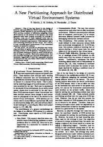
11.2. Amount of Data Sent and Received All the distributed Apriori-T algorithms described involve the exchange of T-tree data. Table 5 shows the average amount of data (in Bytes) sent and received by each process for the different distributed Apriori-T algorithms under consideration assuming five processes. The same data is presented in Figure 4 in the form of two graphs, graphs (a) and (b). Note that:

21

Support (%) 2.0 1.5 1.0 0.5 DATA-DD 18 18 18 24 DATA-TD Ver 1 18 18 18 24 DATA-TD Ver 2 18 18 18 24 DATA-HS 6 6 6 6 DATA-NB 7 7 7 7 DATA-VP 6 6 6 6 Table 4: Number of messages sent, read and taken per process using each of the identified distributed Apriori-T approaches (with 5 processes) for the T20.I10.D500K.N500 dataset •

The figures given in Table 5 are averages; in most cases the range of values making up the average is relatively small and thus the averages are a genuine reflection of the amount of data received and transmitted by each process. The exception to this is the DATA-VP algorithm where the difference between the minimum and maximum may be as much as 0.1Mbytes (see Table 6); this is because the vertical partitioning approach used in DATA-VP does not guarantee an equal division of the work load.

•

With respect to DATA-DD, for each generated T-tree level, un-pruned levels of the T-tree are passed from one process to another (and then pruned).

•

In the case of DATA-TD (both versions) pruned sections of levels in the T-tree are passed from one process to another. Note also that the values obtained for the two versions of DATA-TD are almost identical.

•

DATA-HS and DATA-NB pass a T-tree with a negative border from one process to another. The size of these trees is substantially greater than that of the T-tree containing only frequent sets.

•

For DATA-NB the figures given inc lude the initial T-tree generated and sent in the JavaSpace by the Master process, and read by the Worker processes.

•

DATA-VP passes pruned branches of T-trees (not just levels).

•

Overall, from Table 5, and graphs 4(a) and (b), it can be seen that the amount of data passed between processes when using DATA-VP is significantly less than that associated with any of the other approaches.

Figure 4, graphs (c) and (d) illustrate the amount of data communicated for a support threshold of 0.5, when 3, 5 or 7 processes are used. Here we can see that in the case of the data distribution algorithms, DD, HS and NB, adding more processes increases the amount of communication, because all processes send data to all others. In the case of TD and VP, however, each process sends only the set of candidates it is counting or has counted, which becomes proportionately smaller as the number of processes is increased, so with these methods the messaging overhead remains approximately constant.

22

Support (%) 2.0 1.5 1.0 0.5 DATA-DD 3471888 4621056 8855256 36118584 DATA-TD Ver 1 694896 924480 1771200 7224816 DATA-TD Ver 2 694464 924240 1771152 7224624 DATA-HS 4663408 6343520 13005760 63243808 DATA-NB (worker) 5239404 7128864 14592528 70869816 DATA-VP 10925 21965 59597 228211 Table 5: Average Total size (Bytes) of messages sent and read/taken per process using each of the identified distributed Apriori-T approaches (with 5 processes) for the T20.I10.D500K.N500 dataset

Support threshold (%) 2.0 1.5 1.0 0.5 Master 14144 31184 85040 267248 Worker 1 10288 20464 59296 276064 Worker 2 10064 19424 51760 212944 Worker 3 10064 19376 50976 193232 Worker 4 10064 19376 50912 191568 Averages 10925 21965 59597 228211 Table 6: Size (Bytes) of serialised T-tree messages sent and read/taken per process using the DATAVP approach (with 5 processes) for the T20.I10.D500K.N500 dataset

11.3 Number of Updates The number of support value updates/incrementations per process is a good indication of the amount of work done by each process. Table 7 gives the number of updates for each of the algorithms under consideration for a range of support thresholds and using five processes. The same data is presented in Figure 4(e) in the form of a graph. Note that: •

DATA-DD, DATA-TD (both versions) and DATA-VP all have the same average number of updates (as would be expected).

•

Although the average number of updates for both versions of DATA-TD is the same the range of values making up the average for Version 1 is much greater than that for Version 2, thus demonstrating that the “round robin” distribution of candidate itemsets (Version 2) gives a much better division of the required work than the partition approach (Version 1). This is illustrated in Tables 8 and 9 which show the number of updates required by the DATA-TD algorithm with partition distribution of candidate itemsets and “round robin” distribution of candidate item sets respectively. From Table 8 (DATA-TD Version 1) it can also be seen that in this case the majority of the work is done by the Master process which deals with the most common candidate itemsets.

23

Figure 4: Performance plots for the dataset T20.I10.D500K.N500 •

The range of values associated with DATA-VP entries in Table 7 is also fairly large. This is illustrated in Table 10, whic h gives the number of updates required by the DATA-VP algorithm for this data set. Worker 4 does the least work because the “right most side of the T-tree” (Figure 2) deals with those itemsets that are the least likely to be frequent.

24

•

DATA-HS and DATA-NB have a higher number of updates because of the negative border included in the T-trees, and the reduced support threshold, leading to more sets being counted.

•

The values given for DATA-NB are split into the number of updates carried out by the master process and those by the worker processes. The distinction is that the Master, in this case, process generates the initial T-tree which is then updated by all the processes (master and Workers)

•

Table 7 includes, for comparison, values for the serial form of the Apriori-T algorithm.

In general, the total number of updates is a constant for any support threshold, although this value is grater for methods that use the negative border. This number is divided between the processes, so that each does less work as the number of processes increases. This scaling is illustrated in Figure 4(f). Support (%) 2.0 1.5 1.0 0.5 DATA-DD, DATA-TD, DATA-VP 19779864 22241899 29569327 57080377 DATA-HS 20139564 23325951 33504841 74373312 DATA-NB (Workers) 16847881 19531380 28094029 62828377 DATA-NB (Master) 33383761 38625613 55307786 121706693 Apriori-T (with X-checking) 98899320 111209495 147846636 285401889 Apriori-T (No X-checking 98904425 111248921 147995814 285837823 Table 7: Average number of updates to generate final T-tree per process using each of the identified distributed Apriori-T approaches (with 5 processes) for the T20.I10.D500K.N500 dataset Support threshold (%) 2.0 1.5 1.0 0.5 Master 44428840 51363688 67884086 116334142 Worker 1 21274452 23760010 30900857 56736170 Worker 2 14561747 16119589 21051480 42085942 Worker 3 10716274 11541229 15319608 36006920 Worker 4 7918007 8424979 12690605 34238715 Average 19779864 22241899 29569327 57080377 Table 8: Number of updates per process using the DATA-TD (with Partition Distribution of Candidate Itemsets) approach (with 5 processes) for the T20.I10.D500K.N500 dataset Support threshold (%) 2.0 1.5 1.0 0.5 Master 19973153 22478121 29824163 57409837 Worker 1 20218230 22714102 30102988 57893279 Worker 2 19651582 22068407 29390781 56784577 Worker 3 19719308 22163155 29443052 56960507 Worker 4 19337047 21785710 29085652 56353689 Average 19779864 22241899 29569327 57080377 Table 9: Number of updates per process using the DATA-TD (with “Round Robin” Distribution of Candidate Itemsets) approach (with 5 processes) for the T20.I10.D500K.N500 dataset

25

Support threshold (%) 2.0 1.5 1.0 0.5 Master 21170763 29490310 60748663 113448282 Worker 1 26737796 29711648 36737781 117499445 Worker 2 27279347 29225025 31516143 40066595 Worker 3 24898094 25906678 25620695 24432671 Worker 4 21054340 20014888 17394261 14456772 Table 10: Number of updates per process using the DATA-VP approach (with 5 processes) for the T20.I10.D500K.N500 dataset (maximums highlighted in bold type)

11.4. Execution Time The overall execution time for each algorithm is arguably the most significant performance parameter. A set of times (seconds) is presented in Table 11 (and in graph form in Figures 4(g) and (h)). Note that: •

The table includes, for comparison, execution times using the Apriori-T serial algorithm without X-checking as this provides a slightly better result for this data set (see Table 2).

•

The advantage of Version 2 of the DATA-TD (using “round robin” distribution of candidate sets) in that it offers a more equal distribution of work (see Tables 8 and 9) does not translate into any advantage in execution time. In fact the partition distribution approach is more effective because the candidates allocated to each process are located together in one region of the T-tree, rather than being evenly spread across the T-tree, so less “tree walking” is required using version 1.

Support (%) 2.0 1.5 1.0 0.5 DATA-NB 20 28 49 301 DATA-HS 14 18 36 242 DATA-DD 13 16 25 99 Apriori-T (No X-check) 15 19 31 95 DATA-TD Ver 1 9 9 16 66 DATA-TD Ver 2 11 13 20 77 DATA-VP 3 4 10 31 Table 11: Average execution time(seconds) per process using each of the identified distributed Apriori-T approaches (with 5 processes) for the T20.I10.D500K.N500 dataset

Overall it is clear that the Task Distribution algorithms, DATA-TD, and (especially) the Vertical Partitioning Algorithm DATA-VP perform much better than the data distribution algorithms, DD, HS and NB, in this environment. The reasons for this can be seen in the measurements of messaging overheads for the different methods. The need for each process to transmit and receive a complete T-

26

tree imposes a heavy cost in the DD method, and especially for HS and NB for which a larger tree is created. Conversely, TD and VP transmit (essentially) only the candidates they are counting. The consequences of this can be seen still more clearly in the graphs of Figure 4(i) and (j) which show the scaling of performance as the number of processes varies. The results illustrate that for the DD, HS and NB methods, the increasing overhead of messaging more than outweighs the gain from using additional processes, so the parallelisation is counterproductive. The other methods all show some gain from parallelisation, with DATA-VP giving the best results and the best scaling.

12. SUMMARY AND CONCLUSIONS

In this paper we have described a number of methods for the distribution/parallelisation of the Apriori-T ARM algorithm, using the T-tree set-enumeration structure to contain sets being counted. The advantages and disadvantages of each are summarised in Table 12. Our experimental evaluation of the different approaches clearly demonstrate that, for the datasets chosen and in the context of the implementation environment used, the approaches that use candidate distribution (TD and VP) perform much better than those that distribute the original dataset between processes. This is a because of the high message-passing overheads (in the JavaSpaces environment) associated with the latter. In our experiments, the best results were obtained using the DATA-VP algorithm, which exploits the structure of the T-tree most effectively. The advantages offered by the DATA-VP approach result from the limited number of messages sent and the relatively small content of the messages. This advantage results, in turn, entirely from the nature of the T-tree data structure, which readily supports vertical partitioning of the form described. The results demonstrated in respect of the DATA-VP algor ithm are very encouraging, suggesting that this is a genuinely practical method of parallelising and ARM. We propose further work to examine to what extent the results we have obtained will translate to other parallel processing environments. Some other possible avenues for further work include: 1. Heuristics to achieve a more effective vertical partitioning with respect to the DATA-VP algorithm to provide a more equal distribution of the computational effort required. 2. The effect of including a pre-processing phase using the P-tree data structure (Goulbourne et al. 2000 and Coenen et al. 2003).

27

3. Further experiments to investigate performance varying the number of processors and using different datasets.

DATA-DD

Advantages Disadvantages 1. Allows data to be distributed. 1. Requires several passes through the data 2. 3. 4.

DATA-TD Ver. 1 & 2

1. The content of the message, compared to DATA-DD, is significantly smaller. 2. Efficiency in enhanced as the number of processes increases. 1. Allows data to be distributed. 2. Reduced number of messages compared to DATA-DD and DATA-TD

1.

( longestL arg eItemset + 1 ) The number of messages sent is comparatively large. The size of the messages is also comparatively large --- each representing an entire unpruned Ttree level. Performance deteriorates as the number of processes increases (due to messaging overhead) Also requires several passes through the data

( longestL arg eItemset + 1 ). 2. The number of messages sent is the same as that associated with DATA-DD

1. Multiple passes of the data set, as with DATADD and DATA-TD. 2. The number of nodes in the negative border represents a substantial overhead. 3. Although there are fewer messages the size of the messages is much larger. 4. Performance deteriorates as the number of processes increases (due to messaging overhead) DATA-NB 1. Allows data to be distributed. 1. The required preprocessing to generate the 2. A single pass through the initial T-tree. dataset (excluding the 2. The number of nodes in the negative border generation of the initial Trepresents a substantial overhead. tree). 3. The relatively large message content due to 3. Reduced number of negative border nodes. messages, compared to 4. Performance deteriorates as the number of DATA-DD and DATA-TD. processes increases (due to messaging overhead) amount of 1. The algorithm still requires several passes DATA-VP 1. Minimal messaging as with DATAthrough the dataset. HS 2. All processes require access to full dataset. 2. Minimal message size compared to other approaches. 3. Efficiency in enhanced as the number of processes increases. Table 12: Summary of comparison of Distributed/parallel Apriori-T Algorithms DATA-HS

28

REFERENCES

1. Agarwal, R., Aggarwal, C. and Prasad, V. (2000). A tree projection algorithm for generation of frequent itemsets. J. Parallel and Distributed Computing, 61(3), pp350-371. 2. Agrawal, R, and Shafer, J.C. (1996). Parallel Mining of Association Rules. IEEE Transactions on Knowledge and Data Engineering, Vol 8, No 6, pp962-969.

3. Agrawal, R. and Srikant, A. (1994). Fast algorithms for mining association rules. Proc. VLDB'94, pp487-499. 4. Arnold, K., Freeman, E. and Hupfer, S. (1999). JavaSpaces: Principles, Patterns and Practice. Addison Wesley. 5. Bayardo, R.J. (1998). Efficiently Mining Long Patterns from Datasets. Proc. ACM-SIGMOD, Int. Conf. on Management of Data, ACM Press, pp85-93. 6. Becuzzi, P., Coppola, M. and Vanneschi, M., (1999). Mining of Association Rules in Very Large Databases: A Structured Parallel Approach. Proc. Euro-Par ’99, Lecture Notes in Computer Science 1685, Springer, pp1441-1450 7. Berry, M.J. and Linoff, G.S. (1997). Data Mining Techniques for Marketing, Sales and Customer Support. John Wiley and sons. 8. Brin, S., Motwani, R., Ullman, J. and Tsur, S. (1997). Dynamic Itemset Counting and Implication Rules for Market Basket Data. Proc. ACM-SIGMOD, Int. Conf. On Management of Data, pp255-264. 9. Carreiro, N. and Gelernter, D. (1989). Linda in Context. Communications of the ACM, 32(4). 10. Chattratichat, J., Darlington, J., Ghanem, M., Guo, Y., Hüning, H., Köhler, M., Sutiwaraphun, J., To H. W., Yang, D. (1997). Large Scale Data Mining: Challenges and Responses. proc. 3rd Int.Conf. on Knowledge Discovery and Data mining (KDD'97), pp143-146. 11. Cheung, D., Ng, V., Fu, A., Fu, Y. (1996a). Efficient mining of association rules in distributed databases. IEEE Transactions on Knowledge and data Engineering, IEEE Computer Society Press, pp911-922. 12. Cheung, D., Ng, V., Fu, A., Fu, Y. (1996b). A Fast Distributed Algorithm for Mining Association Rules. Proc. 4th Int Conf. on Parallel and Distributed Information Systems, (PDIS'96), IEEE Computer Society Press, pp31-42. 13. Cheung, D. and Xiao, Y., (1999). Effect of Data Distribution in Parallel Mining of Associations. Data Mining and Knowledge Discovery 3(3), pp 291-314 14. Coenen, F., Goulbourne, G. and Leng, P. (2001). Computing Association Rules Using Partial Totals. Principles of Data Mining and Knowledge Discovery: Proc. 5th European Conference, PKDD 2001, eds. L De Raedt and A Siebes, LNCS, Springer, pp54-66.

29

15. Coenen, F. and Leng, P. (2001). Optimising Association Rule Algorithms Using Itemset Ordering. Research and Development in Intelligent Systems XVIII: Proc. ES2001 Conference, eds M Bramer, F Coenen and A Preece, Springer, pp53-66. 16. Coenen, F., Goulbourne, G. and Leng, P., (2003a). Tree Structures for Mining association Rules. Data Mining and Knowledge Discovery , 8,1, January 2004, pp25-51 17. Coenen, F., Leng, P. and Ahmed, S., (2003b). T-Trees, Vertical Partitioning, and Distributed Association Rule Mining. Proc. IEEE Int. Conf. on Data Mining (ICDM 2003), Florida,

Nov 2003, eds. X Wu, A Tuzhilin and J Shavlik: IEEE Press, pp513-516 18. Goulbourne, G., Coenen, F. and Leng, P. (2000). Algorithms for Computing Association Rules Using a Partial-Support Tree. Journal of Knowledge-Based Systems, Vol (13), pp141149. 19. Han, E.H., Karypis, G. and Kumar, V. (1997). Scalable Parallel Data Mining for Association Rules. Proc. ACM-SIGMOD, Int. Conf. on Management of Data, ACM Press, pp277-288. 20. Han, J., Pei, J. and Yiwen, Y. (2000). Mining Frequent Patterns Without Candidate Generation. Proc. ACM-SIGMOD Int.Conf. on Management of Data, ACM Press, pp1-12. 21. Moore, A. and Lee, M.S. (1998). Cached Sufficient Statistics for Efficient Machine Learning with Large Datasets. Journal of AI Research, pp67-91. 22. Morishita, S. and Nakaya, A. (2000). Parallel branch-and-bound graph search for correlated association rules. In XZaki and Ho (eds.).Large Scale Parallel Data Mining, Lecture Notes in Artificial Intelligence 1759, Springer, pp127-144 23. Park, J.S., Chen, M.S. and Yu, P.S. (1995). An effective hash-base algorithm for mining association rules. Proc. ACM-SIGMOD Int. Conf. on Management of Data, ACM Press, pp175-186. 24. Parthasarathy, S, Zaki, M. and Li, W. (1998). Memory Placement Techniques for Parallel Association Mining. Proc 4th Int. Conf. on Knowledge Discovery in Databases (KDD'98), AAAI Press, pp304-308. 25. Rymon, R. (1992). Search Through Systematic Set Enumeration. Proc. 3rd Int Conf on the Principles of Knowledge and Reasoning, Morgan Kaufman, pp539-550. 26. Shintani, T. and Kitsuregawa, M. (1996). Hash Based Parallel Algorithms for Mining Association Rules. Proc. 4th Int Conf. on Parallel and Distributed Information Systems, (PIDS'96), IEEE Computer Society Press, pp19-30. 27. Tamura, M. and Kitsuregawa, M. (1999). Dynamic Load Balancing for Parallel Association Rule Mining on Heterogeneous PC Cluster Systems. Proc. 25th VLDB Conference, Morgan Kaufman, pp162-173.

30

28. Tan, P.-N., Kumar, V. and Srivastava, J. (2002). Selecting the right interestingness measure for association patterns. Proc. ACM SIGKDD Int. Conf. On Knowledge Discovery and Data Mining (KDD2002), pp32-41. 29. Toivonen, H. (1996). Sampling large databases for association rules. Proc. 22nd VLDB Conference, Morgan Kaufman, pp134-135. 30. Zaki, M.J. (1999). Parallel and Distributed Association Mining: A Survey. IEEE Concurrency, October-December, pp14-25.

31