1, representing a single mast stacker ..... of generating trajectories yf,d which must comply with ... consequence of this parameterization and the fact yf,1 and.
Proceedings of the 17th World Congress The International Federation of Automatic Control Seoul, Korea, July 6-11, 2008
Passivity Based Control and Time Optimal Trajectory Planning of a Single Mast Stacker Crane Martin Staudecker ∗ Kurt Schlacher ∗ Rudolf Hansl ∗∗ ∗
Institute of Automatic Control and Control Systems Technology, Johannes Kepler University Linz, Austria ∗∗ TGW Transportger¨ ate GmbH, Wels, Austria
Abstract: This paper is concerned with feedforward control and active rejection of vibrations of a single mast stacker crane used for the automatic storage or retrieval of load carries in high bay racks. Based on an infinite dimensional mathematical model the trajectory planning and tracking problems are discussed. It turns out that the theory of differential flatness in combination with a finite dimensional approximation of the system is a suitable tool to obtain an open loop control law and to derive time optimal trajectories. The application of backstepping to the infinite dimensional model leads to a passivity based controller for the stabilization of the tracking error. Finally, measurement results show the feasibility of this approach. Keywords: Infinite Dimensional Systems; Flexible Structures; Flatness based Control; Passivity based Control; Trajectory Tracking; Time Optimal Trajectory Planning. 1. INTRODUCTION
x4
In industry a lot of applications are represented by flexible structures, for example stacker cranes operating in a high bay warehouse. The flexibility in such devices arises because of light weight constructions which are preferably used to satisfy the economic objective to increase the efficiency of the storage system. However, this may cause some vibration problems which must be investigated, because they affect storage access time considerably. This contribution deals with a flexible mechanical system as depicted in Fig. 1, representing a single mast stacker crane. Basically, it consists of a driving unit mw which can move only in the X 3 direction. A vertical beam carrying a moving mass mh , in the following also referred to as lifting unit, is attached to this unit. Furthermore, a tip mass mk is fixed at the free end of the beam. The task is to move the mass mh from a starting point into a desired goal equilibrium point inside the (X 1 , X 3 ) plane as fast as possible. To achieve this specification a flatness based feedforward and a passivity based feedback control concept is proposed, see e.g. Macchelli and Melchiorri [2005], Thull et al. [2005]. This paper is organized as follows. In Section 2 an infinite dimensional model of the system is derived. Based on this model trajectory planning is discussed in Section 3. Here we will use the theory of differential flatness applied to a finite dimensional approximation of the nonlinear system to derive an open loop control. A passivity based control law to stabilize the tracking error is proposed next. This will be the main focus of Section 4. Section 5 is concerned with the problem of time optimal trajectory ⋆ This work was supported by our industrial partner TGW Transportger¨ ate GmbH, Wels, Austria.
978-1-1234-7890-2/08/$20.00 © 2008 IFAC
875
mk w(X 1 , t) x3 mh
F2
x2
X1
mw F1
X3 X2 x1
Fig. 1. Mathematical model. generation. The property of differential flatness will help us to formulate a nonlinear parametric optimization program which must be solved to obtain the optimal trajectories. Finally, some measurement results show the feasibility of this approach and complete the contribution.
10.3182/20080706-5-KR-1001.3385
17th IFAC World Congress (IFAC'08) Seoul, Korea, July 6-11, 2008
2. THE MATHEMATICAL MODEL
mw x ¨1 + EI∂x3 w(0, t) = F1 ,
Let us consider the mechanical system shown in Fig. 1. The driving unit is modeled as a rigid body mw with position x1 . The displacement of the beam centerline is denoted by w and we will assume that the beam satisfies the Euler-Bernoulli hypothesis, having length L, uniform mass density ρ, uniform cross section surface A and uniform flexural rigidity EI. The center of gravity of mh moves along the beam center line. As depicted in Fig. 1, the two masses mk and mh can move in the (X 1 , X 3 ) plane with positions x2 , x3 and x4 . The rotary inertia of the beam and of the masses mh and mk are not taken into account. In addition the geometric relations are linearized. The forces F1 and F2 acting on the driving and the lifting unit respectively serve as control inputs. Concerning mathematical notation we will use the shortcuts ∂t = ∂/∂t and ∂x = ∂/∂X 1 as well as ∂tk = ∂ k /∂tk and ∂xk = ∂ k /∂(X 1 )k , k = 2, . . . , n. When dealing with functions u = u(t) we will write u˙ = ∂t u and u ¨ = ∂t2 u for derivatives with respect to the parameter t. Taking into account the assumptions presented above we are able to determine the kinetic energy 1 1 Ekin = mw (x˙ 1 )2 + mh ((x˙ 3 )2 + (x˙ 2 )2 ) + 2 2 Z X1 1 1 2 + mk (x˙ 4 )2 + (∂t w) ρAdX 1 2 X2 2 and the potential and stored elastic energy Z X1 1 Epot = mh gx2 + EI(∂x2 w)2 dX 1 . 2 X2 The contribution of the external forces can be expressed as Eext = x1 F1 + x2 F2 . Hence, the Lagrangian reads as L = Ekin − Epot + Eext and we are able to define the action functional ! Z X1 Z t2 2 1 ¯ x)+ l(∂t w, ∂x w)dX dt L(x, ˙ L= X2
t1
{z
|
L
}
¯ x) whereas L is separated into the function L(x, ˙ and the Lagrangian density l. It still remains to include the restrictions Θ1 = x3 − w(x2 , t) = 0 and Θ2 = x4 − w(L, t) = 0 into the problem formulation. One possibility is to extend the functional L by using the techniques of Lagrange multipliers λ as Z t2 L¯ = L+ λi (t)Θi dt . (1) t1
Here and in the following the Einstein convention for sums is used to keep the formulas short and readable. To derive the equations of motion we apply Hamilton’s principle and get the partial differential equation ρA∂t2 w + EI∂x4 w = 0
(2)
and the ordinary differential equations
876
mh x ¨ 2 + mh g + mh x ¨3 ∂x w(x2 , t) = F2 , EI(∂x3 w(x2− , t) − ∂x3 w(x2+ , t)) = mh x ¨3 ,
(3)
EI∂x3 w(L, t) = mk x ¨4 . Furthermore, the relations w(0, t) = x1 , ∂x w(0, t) = 0, EI(∂x2 w(x2− , t) − ∂x2 w(x2+ , t)) = 0,
(4)
EI∂x2 w(L, t) = 0 must be fulfilled. It is worth mentioning that (2) is valid for the domains Ω1 = [0, x2 ] and Ω2 = [x2 , L] respectively and that (3) correspond to the law of conservation of linear momentum concerning the masses mw , mh and mk . The clamping and the strain conditions at X 1 = 0, X 1 = x2 and X 1 = L are summarized in (4). The values x2+ and x2− denote the right-hand and the left-hand limit of x2 . 3. FLATNESS BASED OPEN LOOP CONTROL Next, the theory of differential flatness, well known and established for finite dimensional nonlinear systems and generalized for a special class of linear infinite dimensional systems, see e.g. Fliess et al. [1995], Rudolph [2003], is used in order to design the feedforward part of the control law. This will be done by means of a finite dimensional system approximation. Therefore, we apply the Ritz ansatz w(X 1 , t) = x1 (t) + Φ1 (X 1 )¯ q 1 (t) (5) for the displacement w with a function in space �2 �3 1 �4 Φ(X 1 ) = 6 X 1 /L − 3 X 1 /L + X 1 /L 2 and the new generalized coordinate q¯1 . The function Φ fulfills the equations (4) but it does not incorporate the shear force condition at X 1 = x2 and X 1 = L. This simplification has been justified by numerical investigations with a higher order ansatz that fulfills this requirement. The substitution of the ansatz into (1) together with Hamilton’s principle leads to the equations of motion Mij (q)¨ q j + Ci (q, q) ˙ q˙ + gi = Gki uk (6) 1 1 2 with i, j = 1, . . . , 3 , k = 1, 2 , q = (x , q¯ , x ) and u = (F1 , F2 ). We get a nonlinear mechanical system underactuated by one control. The elements of the symmetric inertia matrix M and those of the vector C are M12 = m12 + mh Φ(x2 ), ∂Φ(x2 ) M22 = m22 + mh Φ(x2 )2 , M13 = mh q¯1 , ∂x2 ∂Φ(x2 ) M33 = m33 (¯ q 1 , x2 ), M23 = mh q¯1 Φ(x2 ) , ∂x2 � � 2 2 ∂Φ(x2 ) 2 1 ∂ Φ(x ) C1 = mh 2x˙ 2 q¯˙1 , + x ˙ q ¯ ∂x2 ∂(x2 )2 C2 = Φ(x2 )C1 + k1 q¯1 + k2 q¯˙1 , ∂Φ(x2 ) C3 = q¯1 C1 ∂x2
M11 = m11 ,
with constants m11 , m22 , m12 , k1 and k2 . The vectors Gk read as G1 = (1, 0, 0) and G2 = (0, 0, 1). The problem
17th IFAC World Congress (IFAC'08) Seoul, Korea, July 6-11, 2008
is now to find a set of flat outputs (yf1 , yf2 ) for system (6). It is worth mentioning that the explicit state space representation of (6) is not state feedback equivalent to a linear time-invariant system, nevertheless it might be flat. The crucial point is now that the first two rows of (6) can be rewritten as Mij (x2 )¨ q j + Ci1 (x2 , x˙ 2 , x ¨2 )¯ q 1 + Ci2 (x2 , x˙ 2 )q¯˙1 = G1i u1 with i, j = 1, or in explicit first order form as ¨2 )z j + bi (x2 )¯ u (7) z˙ i = Aij (x2 , x˙ 2 , x with i, j = 1, . . . , 4, state vector z = (x1 , x˙ 1 , q¯1 , q¯˙1 ) and the remaining input u ¯ = F1 . Assuming that yf2 = x2 we know the trajectory x2d (t) = yf2 (t) and its time derivatives and thus, we can treat system (7) as a linear time-varying system z˙ i = Aij (x2d , x˙ 2d , x ¨2d )z j + bi (x2d )¯ u. (8) Hence, the construction of a flat output is now straightforward, for example by transformation into time-varying controllability normal form, see e.g. Rothfuß [1997]. A flat output for (8) is given by y¯f = hi (x2d , x˙ 2d , x ¨2d )z i . Because of their complexity the expressions hi are not presented here. Summarizing these observations we propose the differential independent functions yf = (hi (x2 , x˙ 2 , x ¨2 )z i , x2 ) (9) as flat outputs for the original system (6). To show this we succeed in expressing all system variables q and u by yf and its time derivatives which ensures by definition that (9) are indeed flat outputs of the original system (6). Once the flat outputs are found, we are able to calculate an open-loop control by defining a sufficient smooth trajectory yf (t) = yf,d (t). To assure continuous state and input trajectories the function yf1 must be at least four times, the function yf2 at least six times continuously differentiable. To verify this statement it is remarkable that system (6) is linearizable by static state feedback after adding four integrators at input u2 . 4. CONTROLLER DESIGN The aim of this section is to derive a control concept for our elastic structure which provides good tracking behavior and at the same time achieves good disturbance rejection. A frequently used approach is to design the controller for a finite dimensional system approximation. This often leads to undesirable spillover effects in particular when collocation between input and output is not given. To ensure collocation between in- and output we will apply a passivity based approach directly to the infinite dimensional system.
uζe = uζ − uζd
(10)
i
with z = [x , w], u = [F1 , F2 ] and restrict ourself to equilibrium points with constant trajectories for zd and ud .
877
(12)
¨3e , EI(∂x3 we (x2− , t) − ∂x3 we (x2+ , t)) = mh x EI∂x3 we (L, t) = mk x ¨4e and
we (0, t) = x1e , ∂x we (0, t) = 0, EI(∂x2 we (x2− , t)
−
∂x2 we (x2+ , t))
(13)
= 0,
EI∂x2 we (L, t) = 0. According to the total stored energy H = Ekin + Epot a suitable energy functional for the error system is now given by 1 1 1 He = mw (x˙ 1e )2 + mh ((x˙ 3e )2 + (x˙ 2e )2 ) + mk (x˙ 4e )2 2 2 2 Z L 1 1 + (ρA(∂t we )2 + EI(∂x2 we )2 )dX 1 . (14) 2 0 2 The calculation of the time derivative of (14) along a solution of (11) to (13) yields d He = x˙ 1e F1,e + x˙ 2e F2,e . dt Hence, the energy ports of our error system are given by the collocated pairs (F1,e , x˙ 1e ) and (F2,e , x˙ 2e ) and the control law F1,e = −α1 x˙ 1e , F2,e = −α2 x˙ 2e (15) with α1 , α2 > 0 might be applied to provide d He = −α1 (x˙ 1e )2 − α2 (x˙ 2e )2 ≤ 0 . dt It is worth mentioning that here only damping injection is considered. For practical use, in case of unfavorable mass relationships or very strong friction effects at the driving unit, this control law provides a very week disturbance rejection. To avoid this disadvantage we use the method of backstepping to construct a new energy functional which provides an improved control law. This approach was already successfully applied in e.g. d’Andre´a Novel and Coron [2000], Thull et al. [2005] for some well known heavy chain systems. First we start with the splitting of our system as shown in Fig. 2. We obtain the subsystem beam and lifting unit Σ1 x˙ 1 Σ2
Because we are interested in the behavior of the error dynamics we consider the change of coordinates and inputs
(11)
mh x ¨2e + mh x ¨3e ∂x we (x2 , t) = F2,e ,
F1
4.1 Stabilization of an equilibrium point
zei = Ψi (z) = z i − zdi ,
With this transformation the error system reads as ρA∂t2 we + EI∂x4 we = 0 together with mw x ¨1e + EI∂x3 we (0, t) = F1,e ,
x˙ 1
x˙ 2 Σ1
Q
F2
Fig. 2. Energy based system splitting. and the subsystem driving unit Σ2 with the coupling force Q = EI∂x3 w(0, t) which represents the shear force at the
17th IFAC World Congress (IFAC'08) Seoul, Korea, July 6-11, 2008
clamping of the beam. The energy functional of the error subsystem beam and lifting unit is now given by 1 1 HΣ1 = mh ((x˙ 3e )2 + (x˙ 2e )2 ) + mk (x˙ 4e )2 + 2 2 Z 1 L 1 + (ρA(∂t we )2 + EI(∂x2 we )2 )dX 1 . 2 0 2
(16)
Again, taking the time derivative of (16) along a solution of (11) to (13) we obtain d HΣ1 = x˙ 1e Qe + x˙ 2e F2,e . dt Furthermore, we can state that the energy exchange between the two subsystems is done via the port (x˙ 1e , Qe ). To establish stabilization of the positions x1 and x2 , which was not taken into account yet, (16) is extended with the energy of two nonlinear springs, namely Z x1e Z x2e ¯ V e = α 1 HΣ 1 + c1 (ξ)dξ + c2 (ξ)dξ , (17) 0
0
whereas the conditions ci (ξ)ξ > 0 for ξ 6= 0 and ci (0) = 0 must be met. The time derivative of (17) along a solution of the error system yields d ¯ Ve = x˙ 1e (α1 Qe + c1 (x1e )) + dt +x˙ 2e (α1 F2,e + c2 (x2e )) .
Let us consider x˙ 1e as fictive control input of Σ1 , then the control law x˙ 1e = −α1 Qe + c1 (x1e ) , 1 α2 2 F2,e = − c2 (x2e ) − x˙ α1 α1 e d ¯ Ve ≤ 0. To include the with α1 , α2 > 0 would yield dt real control input F1,e , analogously to the backstepping approach for nonlinear finite dimensional systems, the new functional 1 Ve = V¯e + (x˙ 1e + α1 Qe + c1 (x1e ))2 (18) 2 is introduced. Once again differentiating (18) with respect to time along a solution of (11) to (13) yields d Ve = −(α1 Qe + c1 (x1e ))2 + (x˙ 1e + α1 Qe + dt 1 +c1 (x1e ))( (F1,e − Qe ) + α1 Q˙ e + mw dc1 + 1 x˙ 1e ) + x˙ 2e (α1 F¯2,e + c2 (x2e )) . dxe
(19)
where the shortcut Q˙ e = EI∂x3 w˙ e (0, t) is used. Now it is easy to show by substituting in (19), that the control law F1,e = −mw ((α2 + 1) c1 (x1e ) + (α2 + +(α1 + α1 α2 −
dc1 1 )x˙ dx1e e
1 )Qe + α1 Q˙ e ) mw
d Ve = −(α1 Qe + c1 (x1e ))2 − α3 (x˙ 2e )2 − dt −α2 (x˙ 1e + α1 Qe + c1 (x1e ))2
(21)
which provides the desired result d Ve ≤ 0 . dt Now, in contrast to (15), the positions x1 , x2 , the shear force Q and their time derivatives appear in the control law. This means an additional measurement but it will improve the disturbance rejection considerably. In contrast to the finite dimensional case to show stability of an infinite dimensional system in the sense of Lyapunov the conditions Ve > 0 and V˙ e ≤ 0 are only necessary and therefore, further investigations must be done. 4.2 Trajectory tracking The trajectory tracking problem is more challenging because in this case the transformation (10) and consequently the error system become time variant and therefore time variant theory must be taken into account. The derivation of a tracking controller based on the time variant error system is part of future efforts. In this paper we will assume that |y˙ d | is sufficiently small and use the control law (20) as tracking controller. The desired trajectories zdi in (10) are replaced by those of section 3. The feasibility of this assumption is shown by simulation and confirmed with measurement results in section 6. 5. TIME OPTIMAL MOTION PLANNING The previous system analysis tells us that the finite dimensional system representation is differential flat with outputs yf . Hence, we are confronted with the problem of generating trajectories yf,d which must comply with constraints and sometimes it is desirable to have trajectories that provide optimal performance according to some criteria. In our particular case we ask for time optimal trajectories to move the system from an initial into a desired goal equilibrium point as fast as possible but within the system i constraints. These constraints are once velocity vmax , i i acceleration amax and jerk constraints rmax of the driving and the lifting unit respectively. Moreover, we have to constrain the bending moment Mb of the beam at the clamping area because here the highest bending stress occurs. For example, this can be necessary to guarantee fatigue resistance. The limits of the input forces are not taken into account because they are not violated in this setup. 5.1 Problem Formulation
(20)
α3 2 1 c2 (x2e ) − x˙ α1 α1 e with α1 , α2 , α3 > 0 implies F2,e = −
878
At first the outputs are parameterized in terms of B-spline functions. B-splines are frequently used basis functions because of some significant properties, e.g. their ease of enforcing continuity across knot points and ease of computing their derivatives, they are defined locally, etc. A
17th IFAC World Congress (IFAC'08) Seoul, Korea, July 6-11, 2008
detailed discussion of B-splines and their implementation can be found in de Boor [1978]. We get
0 .5
0 .4
x 2 [m ]
yf,2 = Bi2 ,n2 (t)pi22 , yf,1 = Bi1 ,n1 (t)pi11 , i1 = 1, . . . , N1 , i2 = 1, . . . , N2 , whereas Bi,n (t) denotes the B-spline basis function of the i-th knot with order n and p1 , p2 the vectors of parameters to be calculated. As a consequence of this parameterization and the fact yf,1 and yf,2 are flat outputs, the system variables z = [xi , Fi , Mb ] are determined by p1 and p2 , namely z = z(yf,i , ∂tk yf,i ) = z(p1 , p2 , t) with k = 1, . . . , 4. Next, Nc points are chosen uniformly over the time interval [0, Tend ], the constraints will be evaluated at these points. Moreover, we will not directly minimize the end time Tend but instead we will solve a sequence of subproblems each with fixed Tend . The subproblem can now be stated as the following nonlinear programming form: min kF1 (p, tk )k∞ p i 1 1 i ∂t x (p, tk ) ≤ vmax x (p, 0) = x0 2 2 2 i i x (p, 0) = x0 ∂t3 xi (p, tk ) ≤ aimax 1 1 ∂t x (p, tk ) ≤ rmax x (p, Tend ) = xend x2 (p, Tend ) = x2end |Mb (p, tk )| ≤ Mb,max
with i = 1, 2, k = 1, . . . , Nc , parameters p = [p1 , p2 ] and tk ∈ [0, Tend ]. Each subproblem is solved for a fixed Tend . If a solution is found Tend is appropriately reduced and the optimization problem is solved again. This procedure is repeated as long as in the next step no possible solution is found. This iteration determines min(Tend ) and finally the time optimization problem is solved. 5.2 Implementation and Results
The presented algorithm was implemented using C++ programming language. The nonlinear programming solver is chosen out of the NAG C library and is based on the SNOPT package described in Gill et al. [2002]. It uses a sequential quadratic programming (SQP) method and is designed for large-scale constrained optimization problems. Fig. 3 shows the time optimal trajectories for the position of the lifting unit in the X 1 -X 3 plane. Thereby, starting from position A the positions B, C and D were passed through successively. For example, the optimization for run A-B was done with the parameters N1 = 60, N2 = 40 and Nc = 599. In addition to Section 3 we want to constrain the jerk r as well and so the values n1 = 5 and n2 = 7 were chosen. Hence, the number of optimization parameters is 109 and the number of constraints is 2001. The CPU-time to solve one subproblem was about 2s and it took five iterations to find min(Tend ). More details to the several trajectories and their constraints will be presented, together with some measurement results, in the next section. Roughly speaking time optimal trajectories are described by the characteristic that during the acceleration phases the lifting unit is at the lowest possible beam position. Consequently a higher acceleration of the driving unit can be achieved within the same maximal bending moment.
879
B
C
0 .3
D
0 .2
0 .1
0 -0 .1
A 0
0 .1
0 .2
0 .3 x
1
0 .4
[m ]
0 .5
0 .6
0 .7
0 .8
Fig. 3. Time optimal trajectories in the X 1 -X 3 plane. Therefore, if possible every time the lifting unit moves downwards and just at the last feasible moment it moves upwards again to reach the desired goal position.
6. MEASUREMENT RESULTS The time optimal feed forward part together with the control law (20) were implemented at the laboratory experiment. Some setup data of interest are mw = 13.1kg, mh = 0.86kg, L = 0.54m, EI = 15.1Nm and ρA = 1 = 0.8m/s, 2.1kg/m. The constraints are fixed to vmax 2 2 2 1 2 1 vmax = 0.4m/s, amax = 4m/s , amax = 6m/s , rmax = 3 3 2 2m/s , rmax = 6m/s and Mb,max = 0.75Nm. The bending moment is measured via strain gage attached near the clamping of the beam. The shear force which is necessary in the control law could be measured directly by the help of a force sensor. Here it is approximated using the relationship between Mb and Q given by the first order ˆ = Mb (∂x3 Φ(0, t)/∂x2 Φ(0, t)). ansatz (5), namely Q Fig. 4 shows the desired and the measured trajectories of run A-B depicted in Figure 3. The optimal trajectories are calculated in such a way, that despite the motion of the lifting unit, the flexible structure moves from point A to B along the defined constraints. The lifting unit remains at the lowest beam position as long as possible and finally 2 moves upwards with vmax . Furthermore, it can be observed that the trajectories of the driving unit are adapted to the position of mh as well. Here the acceleration is higher and therefore, the duration of this phase is shorter than the braking phase which is much softer. Although the feedback part of the control law is designed for stabilizing an equilibrium point, it turns out that it acts also perfectly together with the feedforward part. The high frequent vibrations that arise in the measured bending moment signal, occur because of mechanical vibrations caused by some friction effects between lifting unit and beam. But it shows the robustness of the proposed control law that in spite of these uncertainties the closed loop is stable.
17th IFAC World Congress (IFAC'08) Seoul, Korea, July 6-11, 2008
1 0.5 position x2 [m]
position x1 [m]
0.8 0.6 0.4 0.2
x1(t)
0
x1d(t) 0
0.5
1
1.5
2
0.4 0.3 0.2 x2(t)
0.1 0
2.5
x2d(t) 0
0.5
1
time [s]
1.5
2
2.5
time [s]
1 v 1(t)
x
0.4
vx1,d(t)
velocity v 2 [m/s]
0.6
vx2,d(t)
0.3
x
velocity vx1 [m/s]
v 2(t)
x
0.8
0.4 0.2
0.2 0.1 0
0 0
0.5
1
1.5
2
−0.1
2.5
0
0.5
1
time [s]
1.5
2
2.5
time [s]
60
F1,d(t)
b
F1(t)
bending moment M [Nm]
force F1 [N]
1 80
40 20 0 −20
0
0.5
1
1.5
2
0.5 0 −0.5
Mb,d(t) −1
2.5
Mb(t)
0
time [s]
0.5
1
1.5
2
2.5
time [s]
Fig. 4. Trajectory tracking performance of the proposed control law. REFERENCES
7. CONCLUSION We have shown that the combination of flatness based feedforward and passivity based feedback control is an appropriate tool to achieve trajectory planning and tracking for a single mast stacker crane as shown in Fig. 1. In particular it is pointed out that the derivation of the open loop control by a finite dimensional system approximation assures good results. To improve disturbance rejection the method of backstepping is used to design a new Lyapunov function and as a consequence of this a new control law, where we successfully integrated the shear force Q. In addition, the property of differential flatness helped us to formulate a nonlinear optimization problem to finally obtain the time optimal trajectories. The measurement results in Fig. 4 show the feasibility of this approach. ACKNOWLEDGEMENTS The authors gratefully acknowledge our industrial partner TGW Transport GmbH for their support during this project.
880
B. d’Andre´a Novel and J.M. Coron. Exponential stabilization of an overhead crane with flexible cable via backstepping approach. Automatica, 36:587–593, 2000. C. de Boor. A Practical Guide to Splines. Springer, New York, 1978. M. Fliess, J. L´evine, P. Martin, and P.Rouchon. Flatness and Defect of Nonlinear Systems: Introductory Theory and Examples. Int. J. Control, 61:1327–1361, 1995. Philip E. Gill, Walter Murray, and Micheal A. Saunders. SNOPT: An SQP Algorithm for large-scale Constrained Optimization. SIAM Journal, 12:979–1006, 2002. A. Macchelli and C. Melchiorri. Modeling and control of the Timoshenko beam. the distributed port Hamiltonian approach. SIAM j. control optim., 43:743–767, 2005. R. Rothfuß. Anwendung der flachheitsbasierten Analyse und Regelung nichtlinearer Mehrgr¨ oßensysteme. VDI Verlag, 1997. J. Rudolph. Flatness Based Control of Distributed Parameter Systems. Shaker, Aachen, 2003. D. Thull, D. Wild, and A. Kugi. Infinit dimensionale Regelung eines Br¨ uckenkrans mit schweren Ketten. atAutomatisierungstechnik, 8:400–410, 2005.