Patch-Based Convolutional Neural Network for Whole Slide Tissue ...

Patch-based Convolutional Neural Network for Whole Slide Tissue Image Classification Le Hou1 , Dimitris Samaras1 , Tahsin M. Kurc2,4 , Yi Gao2,1,3 , James E. Davis5 , and Joel H. Saltz2,1,5,6 1 Dept. of Computer Science, Stony Brook University 2 Dept. of Biomedical Informatics, Stony Brook University 3 Dept. of Applied Mathematics and Statistics, Stony Brook University 4 Oak Ridge National Laboratory 5 Dept. of Pathology, Stony Brook Hospital 6 Cancer Center, Stony Brook Hospital {lehhou,samaras}@cs.stonybrook.edu

{tahsin.kurc,joel.saltz}@stonybrook.edu

{yi.gao,james.davis}@stonybrookmedicine.edu

Abstract Convolutional Neural Networks (CNN) are state-of-theart models for many image classification tasks. However, to recognize cancer subtypes automatically, training a CNN on gigapixel resolution Whole Slide Tissue Images (WSI) is currently computationally impossible. The differentiation of cancer subtypes is based on cellular-level visual features observed on image patch scale. Therefore, we argue that in this situation, training a patch-level classifier on image patches will perform better than or similar to an image-level classifier. The challenge becomes how to intelligently combine patch-level classification results and model the fact that not all patches will be discriminative. We propose to train a decision fusion model to aggregate patch-level predictions given by patch-level CNNs, which to the best of our knowledge has not been shown before. Furthermore, we formulate a novel Expectation-Maximization (EM) based method that automatically locates discriminative patches robustly by utilizing the spatial relationships of patches. We apply our method to the classification of glioma and non-small-cell lung carcinoma cases into subtypes. The classification accuracy of our method is similar to the inter-observer agreement between pathologists. Although it is impossible to train CNNs on WSIs, we experimentally demonstrate using a comparable non-cancer dataset of smaller images that a patch-based CNN can outperform an image-based CNN.

1. Introduction Convolutional Neural Networks (CNNs) are currently the state-of-the-art image classifiers [30, 29, 7, 23]. However, due to high computational cost, CNNs cannot be applied to very high resolution images, such as gigapixel

Whole Slide Tissue Images (WSI). Classification of cancer WSIs into grades and subtypes is critical to the study of disease onset and progression and the development of targeted therapies, because the effects of cancer can be observed in WSIs at the cellular and sub-cellular levels (Fig. 1). Applying CNN directly for WSI classification has several drawbacks. First, extensive image downsampling is required by which most of the discriminative details could be lost. Second, it is possible that a CNN might only learn from one of the multiple discriminative patterns in an image, resulting in data inefficiency. Discriminative information is encoded in high resolution image patches. Therefore, one solution is to train a CNN on high resolution image patches and predict the label of a WSI based on patch-level predictions.

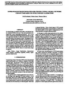
Figure 1: A gigapixel Whole Slide Tissue Image of a grade IV tumor. Visual features that determine the subtype and grade of a WSI are visible in high resolution. In this case, patches framed in red are discriminative since they show typical visual features of grade IV tumor. Patches framed in blue are non-discriminative since they only contain visual features from lower grade tumors. Discriminative patches are dispersed throughout the image at multiple locations. The ground truth labels of individual patches are un12424

known, as only the image-level ground truth label is given. This complicates the classification problem. Because tumors may have a mixture of structures and texture properties, patch-level labels are not necessarily consistent with the image-level label. More importantly, when aggregating patch-level labels to an image-level label, simple decision fusion methods such as voting and max-pooling are not robust and do not match the decision process followed by pathologists. For example, a mixed subtype of cancer such as oligoastrocytoma, might have distinct regions of other cancer subtypes. Therefore, neither voting nor max-pooling could predict the correct WSI-level label since the patchlevel predictions do not match the WSI-level label.

Figure 2: An overview of our workflow. Top: A CNN is trained on patches. An EM-based method iteratively eliminates non-discriminative patches. Bottom: An image-level decision fusion model is trained on histograms of patchlevel predictions, to predict the image-level label. We propose using a patch-level CNN and training a decision fusion model as a two-level model, shown in Fig. 2. The first-level (patch-level) model is an Expectation Maximization (EM) based method combined with CNN that outputs patch-level predictions. In particular, we assume that there is a hidden variable associated with each patch extracted from an image that indicates whether the patch is discriminative (i.e. the true hidden label of the patch is the same as the true label of the image). Initially, we consider

all patches to be discriminative. We train a CNN model that outputs the cancer type probability of each input patch. We apply spatial smoothing to the resulting probability map and select only patches with higher probability values as discriminative patches. We iterate this process using the new set of discriminative patches in an EM fashion. In the second-level (image-level), histograms of patch-level predictions are input into an image-level multiclass logistic regression or Support Vector Machine (SVM) [10] model that predicts the image-level labels. Pathology image classification and segmentation is an active research field. Most WSI classification methods focus on classifying or extracting features on patches [17, 35, 50, 56, 11, 4, 48, 14, 50]. In [50] a pretrained CNN model extracts features on patches which are then aggregated for WSI classification. As we show here, the heterogeneity of some cancer subtypes cannot be captured by those generic CNN features. Patch-level supervised classifiers can learn the heterogeneity of cancer subtypes, if a lot of patch labels are provided [17, 35]. However, acquiring such labels in large scale is prohibitive, due to the need for specialized annotators. As digitization of tissue samples becomes commonplace, one can envision large scale datasets, that could not be annotated at patch scale. Utilizing unlabeled patches has led to Multiple Instance Learning (MIL) based WSI classification [16, 51, 52]. In the MIL paradigm [18, 33, 5], unlabeled instances belong to labeled bags of instances. The goal is to predict the label of a new bag and/or the label of each instance. The Standard Multi-Instance (SMI) assumption [18] states that for a binary classification problem, a bag is positive iff there exists at least one positive instance in the bag. The probability of a bag being positive equals to the maximum positive prediction over all of its instances [6, 54, 27]. Combining MIL with Neural Networks (NN) [43, 57, 31, 13], the SMI assumption is modeled by max-pooling. Following this formulation, the Back Propagation for Multi-Instance Problems (BP-MIP) [43, 57] performs back propagation along the instance with the maximum response if the bag is positive. This is inefficient because only one instance per bag is trained in one training iteration on the whole bag. MIL-based CNNs have been applied to object recognition [38] and semantic segmentation [40] in image analysis – the image is the bag and image-windows are the instances [36]. These methods also follow the SMI assumption. The training error is only propagated through the object-containing window which is also assumed to be the window that has the maximum prediction confidence. This is not robust because one significantly misclassified window might be considered as the object-containing window. Additionally, in WSIs, there might be multiple windows that contain discriminative information. Hence, recent semantic image segmentation approaches [12, 41, 39] smooth the 2425

output probability (feature) maps of the CNNs. To predict the image-level label, max-pooling (SMI) and voting (average-pooling) were applied in [36, 30, 17]. However, it has been shown that in many applications, learning decision fusion models can significantly improve performance compared to voting [42, 45, 24, 47, 26, 46]. Furthermore, such a learned decision fusion model is based on the Count-based Multiple Instance (CMI) assumption which is the most general MIL assumption [49]. Our main contributions in this paper are: (1) To the best of our knowledge, we are the first to combine patch-level CNNs with supervised decision fusion. Aggregating patchlevel CNN predictions for WSI classification significantly outperforms patch-level CNNs with max-pooling or voting. (2) We propose a new EM-based model that identifies discriminative patches in high resolution images automatically for patch-level CNN training, utilizing the spatial relationship between patches. (3) Our model achieves multiple state-of-the-art results classifying WSIs to cancer subtypes on the TCGA dataset. Our results are similar or close to inter-observer agreement between pathologists. Larger classification improvements are observed in the harder-toclassify cases. (4) We provide experimental evidence that combining multiple patch-level classifiers might actually be advantageous compared to whole image classification. The rest of this paper is organized as follows. Sec. 2 describes the framework of the EM-based MIL algorithm. Sec. 3 discusses the identification of discriminative patches. Sec. 4 explains the image-level model that predicts the image-level label by aggregating patch-level predictions. Sec. 5 shows experimental results. The paper concludes in Sec. 6. App. A lists the cancer subtypes in our experiments.

of bag Xi . We further assume that all Xi,j depends on Hi,j only and are independent with each other given Hi,j . Thus P (X, H) =

P (X, H) =

N  Y



P (Xi,1 , . . . , Xi,Ni | Hi )P (Hi ) , (1)

i=1

where the hidden variable H = {H1 , H2 , . . . , HN }, Hi = {Hi,1 , Hi,2 , . . . , Hi,Ni } and Hi,j is the hidden variable that indicates whether instance xi,j is discriminative for label yi

 P (Xi,j | Hi,j )P (Hi ) .

(2)

i=1 j=1

We maximize the data likelihood P (X) using EM. 1. At the initial E step, we set Hi,j = 1 for all i, j. This means that all instances are considered discriminative. 2. M step: We update the model parameter θ to maximize the data likelihood θ ← arg max P (X | H; θ) θ Y P (xi,j , yi | θ) = arg max θ

×

xi,j ∈D

Y

(3)

P (xp,q , yq | θ),

xp,q 6∈D

where D is the discriminative patches set. Assuming a uniform generative model for all non-discriminative instances, the optimization in Eq. 3 simplifies to: Y P (xi,j , yi | θ) arg max θ

= arg max θ

xi,j ∈D

Y

(4) P (yi | xi,j ; θ)P (xi,j | θ).

xi,j ∈D

Additionally we assume an uniform distribution over xi,j . Thus Eq. 4 describes a discriminative model (in this paper we use a CNN). 3. E step: We estimate the hidden variables H. In particular, Hi,j = 1 if and only if P (Hi,j | X) is above a certain threshold. In the case of image classification, given the i-th image, P (Hi,j | X) is obtained by applying Gaussian smoothing on P (yi | xi,j ; θ) (Detailed in Sec 3). This smoothing step utilizes the spatial relationship of P (yi | xi,j ; θ) in the image. We then iterate back to the M step till convergence.

2. EM-based method with CNN An overview of our EM-based method can be found in Fig. 2. We model a high resolution image as a bag and patches extracted from it as instances. We have a ground truth label for the whole image but not for the individual patches. We model whether an instance is discriminative or not as a hidden binary variable. We denote X = {X1 , X2 , . . . , XN } as the dataset containing N bags. Each bag Xi = {Xi,1 , Xi,2 , . . . , Xi,Ni } consists of Ni instances, where Xi,j = hxi,j , yi i is the j-th instance and its associated label in the i-th bag. Assuming the bags are independent and identically distributed (i.i.d.), the X and the hidden variables H are generated by the following generative model:

Ni  N Y Y

Many MIL algorithms can be interpreted through this formulation. Based on the SMI assumption, the instance with the maximum P (Hi,j | X) is the discriminative instance for the positive bag, as in the EM Diverse Density (EM-DD) [55] and the BP-MIP [43, 57] algorithms.

3. Discriminative patch selection Patches xi,j that have P (Hi,j | X) larger than a threshold Ti,j are considered discriminative and are selected to continue training the CNN. We present in this section the estimation of P (H | X) and the choice of the threshold. It is reasonable to assume that P (Hi,j | X) is correlated with P (yi | xi,j ; θ), i.e. patches with lower P (yi | xi,j ; θ) 2426

tend to have lower probability xi,j to be discriminative. However, a hard-to-classify patch, or a patch close to the decision boundary may have low P (yi | xi,j ; θ) as well. These patches are informative and should not be rejected. Therefore, to obtain a more robust P (Hi,j | X), we apply the following two steps: First, we train two CNNs on two different scales in parallel. P (yi | xi,j ; θ) is the averaged prediction of the two CNNs. Second, we simply denoise the probability map P (yi | xi,j ; θ) of each image with a Gaussian kernel to compute P (Hi,j | X). This use of spatial relationships yields more robust discriminative patch identification as shown in the experiments in Sec. 5. Choosing a thresholding scheme carefully yields significantly better performance than a simpler thresholding scheme [39]. We obtain the threshold Ti,j for P (Hi,j | X) as follows: We note Si as the set of P (Hi,j | X) values for all xi,j of the i-th image and Ec as the set of P (Hi,j | X) values for all xi,j of the c-th class. We introduce the imagelevel threshold Hi as the P1 -th percentile of Si and the class-level threshold Ri as the P2 -th percentile of Ec , where P1 and P2 are predefined. The threshold Ti,j is defined as the minimum value between Hi and Ri . There are two advantages of our method. First, by using the image-level threshold, there are at least 1 − P1 percent of patches that are considered discriminative for each image. Second, by using the class-level threshold, the thresholds can be easily adapted to classes with different prior probabilities.

4. Image-level decision fusion model We combine the patch-level classifiers of Sec. 3 to predict the image-level label. We input all patch-level predictions into a multi-class logistic regression or SVM that outputs the image-level label. This decision level fusion method [28] is more robust than max-pooling [45]. Moreover, this method can be thought of as a Count-based Multiple Instance (CMI) learning method with two-level learning [49] which is a more general MIL assumption [20] than the Standard Multiple Instance (SMI) assumption. There are three reasons for combining multiple instances: First, on difficult datasets, we do not want to assign an image-level prediction simply based on a single patchlevel prediction (as is the case of the SMI assumption [18]). Second, even though certain patches are not discriminative individually, their joint appearance might be discriminative. For example, a WSI of the “mixed” glioma, Oligoastrocytoma (see App. A) should be recognized when two single glioma subtypes (Oligodendroglioma and Astrocytoma) are jointly present on the slide possibly on non-overlapping regions. Third, because the patch-level model is never perfect and probably biased, an image-level decision fusion model may learn to correct the bias of patch-level decisions. Because it is unclear at this time whether strongly discriminative features for cancer subtypes exist at whole slide

scale [34], we fuse patch-level predictions without the spatial relationship between patches. In particular, the class histogram of the patch-level predictions is the input to a linear multi-class logistic regression model [8] or an SVM with Radial Basis Function (RBF) kernel [10]. Because a WSI contains at least hundreds of patches, the class histogram is very robust to miss-classified patches. To generate the histogram, we sum up all of the class probabilities given by the patch-level CNN. Moreover, we concatenate histograms from four CNNs models: CNNs trained at two patch scales for two different numbers of iterations. We found in practice that using multiple histograms is robust.

5. Experiments We evaluate our method on two Whole Slide Tissue Images (WSI) classification problems: classification of glioma and Non-Small-Cell Lung Carcinoma (NSCLC) cases into glioma and NSCLC subtypes. Glioma is a type of brain cancer that rises from glial cells. It is the most common malignant brain tumor and the leading cause of cancer-related deaths in people under age 20 [1]. NSCLC is the most common lung cancer, which is the leading cause of cancerrelated deaths overall [3]. Classifying glioma and NSCLC into their respective subtypes and grades is crucial to the study of disease onset and progression in order to provide targeted therapies. The dataset of WSIs used in the experiments part of the public Cancer Genome Atlas (TCGA) dataset [2]. It contains detailed clinical information and the Hematoxylin and Eosin (H&E) stained images of various cancers. The typical resolution of a WSI in this dataset is 100K by 50K pixels. In the rest of this section, we first describe the algorithm we tested then show the evaluation results on the glioma and NSCLC classification tasks.

5.1. Patch extraction and segmentation To train the CNN model, we extract patches of size 500×500 from WSIs (examples in Fig. 3). To capture structures at multiple scales, we extract patches from 20X (0.5 microns per pixel) and 5X (2.0 microns per pixel) objective magnifications. We discard patches with less than 30% tissue sections or have too much blood. We extract around 1000 valid patches per image per scale. In most cases the patches are non-overlapping given WSI resolution. To prevent the CNN from overfitting, we perform three kinds of data augmentation in every iteration. We select a random 400×400 sub-patch from each 500×500 patch. We randomly rotate and mirror the sub-patch. We randomly adjust the amount of Hematoxylin and eosin stained on the tissue. This is done by decomposing the RGB color of the tissue into the H&E color space [44], followed by multiplying the magnitude of H and E of every pixel by two i.i.d. Gaussian random variables with expectation equal to one. 2427

(a) GBM

(b) OD

(c) OA

(d) DA

(e) SCC

(f) ADC

Figure 3: Some 20X sample patches of gliomas and Non-Small-Cell Lung Carcinoma (NSCLC) from the TCGA dataset. Two patches in each column belong to the same subtype of cancer. Notice the large intra-class heterogeneity.

5.2. CNN architecture

1. CNN-Vote: CNN followed by voting (averagepooling). We use all patches extracted from a WSI to train the patch-level CNN. There is no second-level model. Instead, the predictions of all patches vote for the final predicted label of a WSI.

The architecture of our CNN is shown in Tab. 1. We used the CAFFE tool box [25] for the CNN implementation. The network was trained on a single NVidia Tesla K40 GPU. Layer Filter size, stride Output W×H×N Input 400 × 400 × 3 Conv 10 × 10, 2 196 × 196 × 80 ReLU+LRN 196 × 196 × 80 Max-pool 6 × 6, 4 49 × 49 × 80 Conv 5 × 5, 1 45 × 45 × 120 ReLU+LRN 45 × 45 × 120 Max-pool 3 × 3, 2 22 × 22 × 120 Conv 3 × 3, 1 20 × 20 × 160 ReLU 20 × 20 × 160 Conv 3 × 3, 1 18 × 18 × 200 ReLU 18 × 18 × 200 Max-pool 3 × 3, 2 9 × 9 × 200 FC 320 ReLu+Drop 320 FC 320 ReLu+Drop 320 FC Dataset dependent Softmax Dataset dependent Table 1: The architecture of our CNN used in glioma and NSCLC classification. ReLU+LRN is a sequence of Rectified Linear Units (ReLU) followed by Local Response Normalization (LRN). Similarily, ReLU+Drop is a sequence of ReLU followed by dropout. The dropout probability is 0.5.

2. CNN-SMI: CNN followed by max-pooling. Same as CNN-Vote except the final predicted label of a WSI equals to the predicted label of the patch with maximum probability over all other patches and classes. 3. CNN-Fea-SVM: We apply feature fusion instead of decision level fusion. In particular, we aggregate the outputs of the second fully connected layer of the CNN on all patches by 3-norm pooling [50]. Then an SVM with RBF kernel predicts the image-level label. 4. EM-CNN-Vote/SMI, EM-CNN-Fea-SVM: EM-based method with CNN-Vote, CNN-SMI, CNN-Fea-SVM respectively. We train the patch-level EM-CNN on discriminative patches identified by the E-step. Depending on the dataset, the discriminative threshold P1 for each image ranges from 0.18 to 0.25; the discriminative threshold P2 for each class ranges from 0.05 to 0.28 (details in Sec. 3). In each M-step, we train the CNN on all the discriminative patches for 2 epochs. 5. EM-Finetune-CNN-Vote/SMI: Similar to EM-CNNVote/SMI except that instead of training a CNN from scratch, we fine-tune a pretrained 16-layer CNN model [46] by training it on discriminative patches. 6. CNN-LR: CNN followed by logistic regression. Same as CNN-Vote except that we train a second-level multiclass logistic regression to predict the image-level label. One tenth of the patches in each image is held out from the CNN to train the second-level multi-class logistic regression.

5.3. Experiment setup The WSIs of 80% of the patients are randomly selected to train the model and the remaining 20% to test. Depending on method, training patches are further divided into i) CNN and ii) decision fusion model training sets. We separate the data twice and average the results. Tested algorithms are:

7. CNN-SVM: CNN followed by SVM with RBF kernel instead of logistic regression. 2428

8. EM-CNN-LR/SVM: EM-based method with CNN-LR and CNN-SVM respectively. 9. EM-CNN-LR w/o spatial smoothing: We do not apply Gaussian smoothing to estimate P (H | X). Otherwise similar to EM-CNN-LR. 10. EM-Finetune-CNN-LR/SVM: Similar to EM-CNNLR/SVM except that instead of training a CNN from scratch, we fine-tune a pretrained 16-layer CNN model [46] by training it on discriminative patches. 11. SMI-CNN-SMI: CNN with max-pooling at both discriminative patch identification and image-level prediction steps. For the patch-level CNN training, in each WSI only one patch with the highest confidence is considered discriminative. 12. NM-LBP: We extract Nuclear Morphological features [15] and rotation invariant Local Binary Patterns [37] from all patches. We build a Bag-of-Words (BoW) [19, 53] feature using k-means followed by SVM with RBF kernel [10], as a non-CNN baseline. 13. Pretrained-CNN-Fea-SVM: Similar to CNN-FeaSVM. But instead of training a CNN, we use a pretrained 16-layer CNN model [46] to extract features from patches. Then we select the top 500 features according to accuracy on the training set [50]. 14. Pretrained-CNN-Bow-SVM: We build a BoW model using k-means on features extracted by the pretrained CNN, followed by SVM [50].

5.4. WSI of glioma classification There are WSIs of six subtypes of glioma in the TCGA dataset [2]. The numbers of WSIs and patients in each class are shown in Tab. 2. All classes are described in App. A. Gliomas GBM OD OA DA AA AO # patients 209 100 106 82 29 13 # WSIs 510 206 183 114 36 15 Table 2: The numbers of WSIs and patients in each class from the TCGA dataset. Class descriptions are in App. A. The results of our experiments are shown in Tab. 3. The confusion matrix is given in Tab. 4. An experiment showed that the inter-observer agreement of two experienced pathologists on a similar dataset was approximately 70% and that even after reviewing the cases together, they agreed only around 80% of the time [22]. Therefore, our accuracy of 77% is similar to inter-observer agreement. In the confusion matrix, we note that the classification accuracy between GBM and Low-Grade Glioma (LGG) is 97% (chance was 51.3%). A fully supervised method achieved 85% accuracy using a domain specific algorithm trained on ten manually labeled patches per class [35]. Our

Methods Acc mAP CNN-Vote 0.710 0.812 CNN-SMI 0.710 0.822 CNN-Fea-SVM 0.688 0.790 EM-CNN-Vote 0.733 0.837 EM-CNN-SMI 0.719 0.823 EM-CNN-Fea-SVM 0.686 0.790 EM-Finetune-CNN-Vote 0.719 0.817 EM-Finetune-CNN-SMI 0.638 0.758 CNN-LR 0.752 0.847 CNN-SVM 0.697 0.791 EM-CNN-LR 0.771 0.845 EM-CNN-LR w/o spatial smoothing 0.745 0.832 EM-CNN-SVM 0.730 0.818 EM-Finetune-CNN-LR 0.721 0.822 EM-Finetune-CNN-SVM 0.738 0.828 SMI-CNN-SMI 0.683 0.765 NM-LBP 0.629 0.734 Pretrained CNN-Fea-SVM 0.733 0.837 Pretrained-CNN-Bow-SVM 0.667 0.756 Chance 0.513 0.689 Table 3: Glioma classification results. The proposed EMCNN-LR method achieved the best result, close to interobserver agreement between pathologists. (Sec. 5.4 ). Predictions Ground Truth GBM OD OA DA AA AO GBM 214 0 2 0 1 0 OD 1 47 22 2 0 1 OA 1 18 40 8 3 1 DA 3 9 6 20 0 1 AA 3 2 3 3 4 0 AO 2 2 3 0 0 1 Table 4: Confusion matrix of glioma classification. The nature of Oligoastrocytoma causes the most confusions. See Sec. 5.4 for details. method is the first to classify five LGG subtypes automatically, a much more challenging classification task than the benchmark GBM vs. LGG classification. We achieve 57.1% LGG-subtype classification accuracy with chance at 36.7%. Most of the confusions are related to oligoastrocytoma (OA) since it is a mixed glioma that is challenging for pathologists to agree on, according to a neuropathology study: “Oligoastrocytomas contain distinct regions of oligodendroglial and astrocytic differentiation... The minimal percentage of each component required for the diagnosis of a mixed glioma has been debated, resulting in poor interobserver reproducibility for this group of neoplasms.” [9]. We compare recognition rates for the OA subtype. The F-score of OA recognition is 0.426, 0.482, and 0.544 using PreCNN-Fea-SVM, CNN-LR, and EM-CNN-LR respectively. We thus see that the improvement over other methods 2429

GBM GBM OD OA WSIs

Pathologist

Max-pooling

EM

Figure 4: Examples of discriminative patch (region) segmentation (best viewed in color). Discriminative regions are indicated in red. Diagnostic or highly discriminative regions are yellow. Non-discriminative regions are in black. Pathologist: ground truth by a pathologist. Max-pooling: results by CNN with the SMI assumption (SMI-CNN-SMI). The discriminative patches are indicated by red arrows. EM: results by our EM-based patch-level CNN (EM-CNNVote/SMI/LR). Notice that max-pooling does not segment enough discriminative regions. becomes increasingly more significant using our proposed method on the harder-to-classify classes. The discriminative patch (region) segmentation results in Fig. 4 demonstrate the quality of our EM-based method.

5.5. WSI of NSCLC classification We use three major subtypes of Non-Small-Cell Lung Carcinoma (NSCLC). Numbers of WSIs and patients in each class are in Tab. 5. All classes are listed in App. A. NSCLCs SCC ADC ADC-mix # patients 316 250 75 # WSIs 347 291 80 Table 5: The numbers of WSIs and patients in each class from the TCGA dataset. Class descriptions are in App. A. Experimental results are shown in Tab. 6; the confusion matrix is in Tab. 7. When classifying SCC vs. non-SCC, inter-observer agreement between pulmonary pathology experts and between community pathologists measured by Cohen’s kappa is κ = 0.64 and κ = 0.41 respectively [21]. We achieved κ = 0.75. When classifying ADC vs. nonADC, the inter-observer agreement between experts and between community pathologists are κ = 0.69 and κ = 0.46 respectively [21]. We achieved κ = 0.60. Therefore, our

Methods Acc mAP CNN-Vote 0.702 0.838 CNN-SMI 0.731 0.852 CNN-Fea-SVM 0.637 0.793 EM-CNN-Vote 0.714 0.842 EM-CNN-SMI 0.731 0.850 EM-CNN-Fea-SVM 0.637 0.791 EM-Finetune-CNN-Vote 0.773 0.877 EM-Finetune-CNN-SMI 0.729 0.853 CNN-LR 0.727 0.845 CNN-SVM 0.738 0.856 EM-CNN-LR 0.743 0.856 EM-CNN-SVM 0.759 0.869 EM-Finetune-CNN-LR 0.784 0.883 EM-Finetune-CNN-SVM 0.798 0.889 SMI-CNN-SMI 0.531 0.749 Pretrained CNN-Fea-SVM 0.778 0.879 Pretrained-CNN-Bow-SVM 0.759 0.871 Chance 0.484 0.715 Table 6: NSCLC classification results. The proposed EMCNN-SVM and EM-Finetune-CNN-SVM achieved best results, close to the inter-observer agreement between pathologists. See Sec. 5.5 for details. Predictions Ground Truth SCC ADC ADC-mix SCC 199 26 0 ADC 30 155 11 ADC-mix 2 25 17 Table 7: The confusion matrix of NSCLC classification. results appear close to inter-observer agreement. The ADC-mix subtype is hard to classify because it contains visual features of multiple NSCLC subtypes. The Pretrained CNN-Fea-SVM method achieves an F-score of 0.412 recognizing ADC-mix cases, whereas our proposed method EM-Finetune-CNN-SVM achieves 0.472. Consistent with the glioma results, our method’s performance advantages are more pronounced in the hardest cases.

5.6. Rail surface defect severity grade classification We evaluate our approach beyond classification of pathology images. A CNN cannot be applied to gigapixel images directly because of computational limitations. Even when the images are small enough for CNNs, our patchbased method compares favorably to an image-based CNN if discriminative information is encoded in image patch scale and dispersed throughout the images. We classify the severity grade of rail surface defects. Automatic defect grading can obviate the need for laborious examination and grading of rail surface defects on a regular basis. We used a dataset [32] of 939 rail surface images with defect severity grades from 0 to 7. Typical image resolution 2430

(a) Grade 0

(b) Grade 2

(c) Grade 4

(d) Grade 7

Figure 5: Sample images of rail surfaces. The grade indicates defect severity. Notice that the defects are in image patch scale and dispersed throughout the image. is 1200×500, as in Fig. 5. To support our claim, we tested two additional methods: 1. CNN-Image: We apply the CNN on image scale directly. In particular, we train the CNN on 400×400 regions randomly extracted from images in each iteration. At test time, we apply the CNN on five regions (top left, top right, bottom left, bottom right, center) and average the predictions. 2. Pretrained CNN-ImageFea-SVM: We apply a pretrained 16-layer network [46] to rail surface images to extract features, and train an SVM on these features. The CNN used in this experiment has a similar achitecture to the one described in Tab. 1 with smaller and fewer filters. The size of patches in our patch-based methods is 64 by 64. We apply 4-fold cross-validation and show the averaged results in Tab. 8. Our patch-based methods EM-CNNSVM and EM-CNN-Fea-SVM outperform the conventional image-based method CNN-Image. Moreover, results using CNN features extracted on patches (Pretrained CNN-FeaSVM) are better than results with CNN features extracted on images (Pretrained-CNN-ImageFea-SVM).

6. Conclusions We presented a patch-based Convolutional Neural Network (CNN) model with a supervised decision fusion model that is successful in Whole Slide Tissue Image (WSI) classification. We proposed an Expectation-Maximization (EM) based method that identifies discriminative patches automatically for CNN training. With our algorithm, we can classify subtypes of cancers given WSIs of patients with accuracy similar or close to inter-observer agreements between pathologists. Furthermore, we experimentally demonstrate using a comparable non-cancer dataset of smaller images, that the performance of our patch-based CNN compare favorably to that of an image-based CNN. In the future we will leverage the non-discriminative patches

Methods Acc mAP CNN-Vote 0.695 0.823 CNN-SMI 0.700 0.801 CNN-Fea-SVM 0.822 0.903 EM-CNN-Vote 0.683 0.817 EM-CNN-SMI 0.684 0.799 EM-CNN-Fea-SVM 0.830 0.908 CNN-LR 0.764 0.867 CNN-SVM 0.803 0.886 EM-CNN-LR 0.772 0.871 EM-CNN-SVM 0.813 0.895 SMI-CNN-SMI 0.258 0.461 Pretrained CNN-Fea-SVM 0.808 0.894 CNN-Image 0.770 0.876 Pretrained CNN-ImageFea-SVM 0.778 0.878 Chance 0.228 0.438 Table 8: Rail surface defect severity grade classification results. Our patch-based method EM-CNN-SVM and EMCNN-Fea-SVM outperform image-based methods CNNImage and Pretrained CNN-ImageFea-SVM significantly. as part of the data likelihood in the EM formulation. We will optimize CNN-training so that it scales up to larger scale pathology datasets.

Acknowledgment This work was supported in part by 1U24CA18092401A1 from the National Cancer Institute, R01LM01111901 and R01LM009239, and partially supported by NSF IIS1161876, IIS-1111047, FRA DTFR5315C00011, the Subsample project from DIGITEO Institute, France, and a gift from Adobe Corp. We thank Ke Ma for providing the rail surface dataset.

Appendix A. Description of cancer subtypes GBM Glioblastoma, ICD-O 9440/3, WHO grade IV. A Whole Slide Image (WSI) is classified as GBM iff one patch can be classified as GBM with high confidence. OD Oligodendroglioma, ICD-O 9450/3, WHO grade II. OA Oligoastrocytoma, ICD-O 9382/3, WHO grade II; Anaplastic oligoastrocytoma, ICD-O 9382/3, WHO grade III. This mixed glioma subtype is hard to classify even by pathologists [22]. DA Diffuse astrocytoma, ICD-O 9400/3, WHO grade II. AA Anaplastic astrocytoma, ICD-O 9401/3, WHO grade III. AO Anaplastic oligodendroglioma, ICD-O 9451/3, WHO grade III. LGG Low-Grade-Glioma. Include OD, OA, DA, AA, AO. SCC Squamous cell carcinoma, ICD-O 8070/3. ADC Adenocarcinoma, ICD-O 8140/3. ADC-mix ADC with mixed subtypes, ICD-O 8255/3. 2431

References http://www.abta.org/ [1] Brain tumor statistics. about-us/news/brain-tumor-statistics/. 4 [2] The cancer genome atlas. https://tcga-data.nci. nih.gov/tcga/. 4, 6 [3] Non-small-cell lung carcinoma. http://www.cancer. org/cancer/lungcancer-non-smallcell/. 4 [4] D. Altunbay, C. Cigir, C. Sokmensuer, and C. GunduzDemir. Color graphs for automated cancer diagnosis and grading. J Biomed Eng, 2010. 2 [5] J. Amores. Multiple instance classification: Review, taxonomy and comparative study. AIJ, 2013. 2 [6] S. Andrews, I. Tsochantaridis, and T. Hofmann. Support vector machines for multiple-instance learning. In NIPS, 2002. 2 [7] Y. Bengio, A. Courville, and P. Vincent. Representation learning: A review and new perspectives. PAMI, 2013. 1 [8] C. M. Bishop et al. Pattern recognition and machine learning. 2006. 4 [9] D. J. Brat, R. A. Prayson, T. C. Ryken, and J. J. Olson. Diagnosis of malignant glioma: role of neuropathology. Journal of neuro-oncology, 2008. 6 [10] C.-C. Chang and C.-J. Lin. Libsvm: a library for support vector machines. TIST, 2011. 2, 4, 6 [11] H. Chang, Y. Zhou, A. Borowsky, K. Barner, P. Spellman, and B. Parvin. Stacked predictive sparse decomposition for classification of histology sections. IJCV, 2014. 2 [12] L.-C. Chen, G. Papandreou, I. Kokkinos, K. Murphy, and A. L. Yuille. Semantic image segmentation with deep convolutional nets and fully connected crfs. arXiv, 2014. 2 [13] Z. Chen, Z. Chi, H. Fu, and D. Feng. Multi-instance multilabel image classification: A neural approach. Neurocomputing, 2013. 2 [14] D. C. Cires¸an, A. Giusti, L. M. Gambardella, and J. Schmidhuber. Mitosis detection in breast cancer histology images with deep neural networks. In MICCAI. 2013. 2 [15] L. A. Cooper, J. Kong, D. A. Gutman, F. Wang, J. Gao, C. Appin, S. Cholleti, T. Pan, A. Sharma, L. Scarpace, et al. Integrated morphologic analysis for the identification and characterization of disease subtypes. JAMIA, 2012. 6 [16] E. Cosatto, P.-F. Laquerre, C. Malon, H.-P. Graf, A. Saito, T. Kiyuna, A. Marugame, and K. Kamijo. Automated gastric cancer diagnosis on h&e-stained sections; ltraining a classifier on a large scale with multiple instance machine learning. In Medical Imaging, 2013. 2 [17] A. Cruz-Roa, A. Basavanhally, F. Gonz´alez, H. Gilmore, M. Feldman, S. Ganesan, N. Shih, J. Tomaszewski, and A. Madabhushi. Automatic detection of invasive ductal carcinoma in whole slide images with convolutional neural networks. In Medical Imaging, 2014. 2, 3 [18] T. G. Dietterich, R. H. Lathrop, and T. Lozano-P´erez. Solving the multiple instance problem with axis-parallel rectangles. AIJ, 1997. 2, 4 [19] L. Fei-Fei and P. Perona. A bayesian hierarchical model for learning natural scene categories. In CVPR, 2005. 6 [20] J. Foulds and E. Frank. A review of multi-instance learning assumptions. Knowl Eng Rev, 2010. 4

[21] J. E. Grilley-Olson, D. T. Moore, K. O. Leslie, B. F. Qaqish, X. Yin, M. A. Socinski, T. E. Stinchcombe, L. B. Thorne, T. C. Allen, P. M. Banks, et al. Validation of interobserver agreement in lung cancer assessment: hematoxylin-eosin diagnostic reproducibility for non-small cell lung cancer: the 2004 world health organization classification and therapeutically relevant subsets. Archives of pathology & laboratory medicine, 2013. 7 [22] M. Gupta, A. Djalilvand, and D. J. Brat. Clarifying the diffuse gliomas an update on the morphologic features and markers that discriminate oligodendroglioma from astrocytoma. AJCP, 2005. 6, 8 [23] K. He, X. Zhang, S. Ren, and J. Sun. Delving deep into rectifiers: Surpassing human-level performance on imagenet classification. In ICCV, 2015. 1 [24] M. Hoai and A. Zisserman. Improving human action recognition using score distribution and ranking. In ACCV. 2014. 3 [25] Y. Jia, E. Shelhamer, J. Donahue, S. Karayev, J. Long, R. Girshick, S. Guadarrama, and T. Darrell. Caffe: Convolutional architecture for fast feature embedding. arXiv, 2014. 5 [26] A. Karpathy, G. Toderici, S. Shetty, T. Leung, R. Sukthankar, and L. Fei-Fei. Large-scale video classification with convolutional neural networks. In CVPR, 2014. 3 [27] M. Kim and F. Torre. Gaussian processes multiple instance learning. In ICML, 2010. 2 [28] M. M. Kokar, J. A. Tomasik, and J. Weyman. Data vs. decision fusion in the category theory framework. 2001. 4 [29] A. Krizhevsky, I. Sutskever, and G. E. Hinton. Imagenet classification with deep convolutional neural networks. In NIPS, 2012. 1 [30] Y. LeCun, L. Bottou, Y. Bengio, and P. Haffner. Gradientbased learning applied to document recognition. Proceedings of the IEEE, 1998. 1, 3 [31] C. H. Li, I. Gondra, and L. Liu. An efficient parallel neural network-based multi-instance learning algorithm. J Supercomput, 2012. 2 [32] K. Ma, T. F. Y. Vicente, D. Samaras, M. Petrucci, and D. L. Magnus. Texture classification for rail surface condition evaluation. In WACV, 2016. 7 [33] O. Maron and T. Lozano-P´erez. A framework for multipleinstance learning. NIPS, 1998. 2 [34] S. E. Mills. Histology for pathologists. Lippincott Williams & Wilkins, 2012. 4 [35] H. S. Mousavi, V. Monga, G. Rao, and A. U. Rao. Automated discrimination of lower and higher grade gliomas based on histopathological image analysis. JPI, 2015. 2, 6 [36] M. H. Nguyen, L. Torresani, F. De La Torre, and C. Rother. Weakly supervised discriminative localization and classification: a joint learning process. In ICCV, 2009. 2, 3 [37] T. Ojala, M. Pietikainen, and T. Maenpaa. Multiresolution gray-scale and rotation invariant texture classification with local binary patterns. PAMI, 2002. 6 [38] M. Oquab, L. Bottou, I. Laptev, and J. Sivic. Weakly supervised object recognition with convolutional neural networks. In NIPS. 2

2432

[39] G. Papandreou, L.-C. Chen, K. Murphy, and A. L. Yuille. Weakly-and semi-supervised learning of a dcnn for semantic image segmentation. arXiv, 2015. 2, 4 [40] D. Pathak, E. Shelhamer, J. Long, and T. Darrell. Fully convolutional multi-class multiple instance learning. arXiv, 2014. 2 [41] P. O. Pinheiro and R. Collobert. Weakly supervised semantic segmentation with convolutional networks. arXiv, 2014. 2 [42] S. Poria, E. Cambria, and A. Gelbukh. Deep convolutional neural network textual features and multiple kernel learning for utterance-level multimodal sentiment analysis. 3 [43] J. Ramon and L. De Raedt. Multi instance neural networks. 2000. 2, 3 [44] A. C. Ruifrok and D. A. Johnston. Quantification of histochemical staining by color deconvolution. Anal Quant Cytol Histol, 2001. 4 [45] A. Seff, L. Lu, K. M. Cherry, H. R. Roth, J. Liu, S. Wang, J. Hoffman, E. B. Turkbey, and R. M. Summers. 2d view aggregation for lymph node detection using a shallow hierarchy of linear classifiers. In MICCAI. 2014. 3, 4 [46] K. Simonyan and A. Zisserman. Very deep convolutional networks for large-scale image recognition. CoRR, 2014. 3, 5, 6, 8 [47] F. Tabib Mahmoudi, F. Samadzadegan, and P. Reinartz. a decision level fusion method for object recognition using multi-angular imagery. International Archives of the Photogrammetry, Remote Sensing and Spatial Information Sciences, 2013. 3 [48] T. H. Vu, H. S. Mousavi, V. Monga, U. Rao, and G. Rao. Dfdl: Discriminative feature-oriented dictionary learning for histopathological image classification. arXiv, 2015. 2 [49] N. Weidmann, E. Frank, and B. Pfahringer. A two-level learning method for generalized multi-instance problems. In ECML. 2003. 3, 4 [50] Y. Xu, Z. Jia, Y. Ai, F. Zhang, M. Lai, E. I. Chang, et al. Deep convolutional activation features for large scale brain tumor histopathology image classification and segmentation. In ICASSP, 2015. 2, 5, 6 [51] Y. Xu, T. Mo, Q. Feng, P. Zhong, M. Lai, E. I. Chang, et al. Deep learning of feature representation with multiple instance learning for medical image analysis. In ICASSP, 2014. 2 [52] Y. Xu, J.-Y. Zhu, I. Eric, C. Chang, M. Lai, and Z. Tu. Weakly supervised histopathology cancer image segmentation and classification. Medical image analysis, 2014. 2 [53] J. Yang, Y.-G. Jiang, A. G. Hauptmann, and C.-W. Ngo. Evaluating bag-of-visual-words representations in scene classification. In Workshop on multimedia information retrieval, 2007. 6 [54] C. Zhang, J. C. Platt, and P. A. Viola. Multiple instance boosting for object detection. In NIPS, 2005. 2 [55] Q. Zhang and S. A. Goldman. Em-dd: An improved multiple-instance learning technique. In NIPS, 2001. 3 [56] Y. Zhou, H. Chang, K. Barner, P. Spellman, and B. Parvin. Classification of histology sections via multispectral convolutional sparse coding. In CVPR, 2014. 2

[57] Z.-H. Zhou and M.-L. Zhang. Neural networks for multiinstance learning. In ICIIT, 2002. 2, 3

2433