Path Availability in Ad Hoc Network Dan Yu, Hui Li and Ingo Gruber Siemens AG, ICM N PG SP RC FR Gustav-Heinemann-Ring 115, 81730 München, Germany Email:
[email protected], Tel. +49 89 636 45507, Fax: +49 89 636 45591
Abstract. Due to the complexity and high randomness, most current researches on ad hoc networks are based on simulation results and empirical analysis, lacking theoretical understanding of the ad hoc networks and their behavior. This paper presents a general ad hoc network model and derives the statistic results of link and path availability properties in ad hoc network. Simulation results are given to verify our theory. This study could serve as groundwork for further ad hoc network researches including ad hoc network performance analysis and routing algorithms design.
1
Introduction
Ad hoc radio network has many advantages over traditional cellular wireless network [1] [2]. It does not require infrastructures and promises greater flexibility, lower operating cost, higher throughput, and better coverage. However, the design of ad hoc networks is a difficult task because of continuous change of network topology and many network parameters that are highly random and highly dependent on each other. Because of the complexity of ad hoc networks, current researches mainly focus on using simulations tools. However, our opinion is that besides simulation, it is still necessary to do theoretical analysis in order to get deep understanding of statistic properties of mobile wireless ad-hoc network, e.g. network connectivity, network capacity and link availability. In this paper, we emphasize on the analysis of link and route availability properties of ad hoc networks. Throughout this paper, our definition of link availability is the probability that a wireless link between two mobile nodes remain exist after a given time t. Link availability may be taken into account in path selection and path update in routing algorithms to achieve better performance. In an ad hoc network, link availability is extended to path availability, which means the probability that a multihop path is available after a certain time. In [3] link and path availability models for wireless ad hoc networks with a random walk-based mobility were derived. Based on this mobility model, each node’s movement consists of a sequence of random length intervals called mobility epochs during which a node moves in a constant direction at a constant speed. The speed and direction of each node varies randomly from epoch to epoch. The epoch lengths are exponentially distributed. The speed during each epoch is a random variable of Gaussian distribution, while the direction of the mobile during each epoch is uniformly distributed over [0, 2π). The paper compared analytic and simulated results and
2
Dan Yu, Hui Li and Ingo Gruber
concluded that the relative error increases with increasing path length for small values of epochs. In this paper, we derived link and path availability models for ad-hoc networks with a random walk mobility model that is different from the one in [3]. Our availability study will provide detail insight into the link and path available time and other availability properties in a general ad hoc network. The knowledge of link availability can serve as groundwork for further analysis of network performance, as well as guide to ad hoc network protocol design. The paper is structured as this. First we give a description of our simplified ad hoc network model. The model is applied to our availability analysis, which outlines link available time distribution and link availability and multihop path availability properties. Eventually, simulation results on average link available time are given to verify our theory. The simulation results clearly demonstrated the correctness of our analytical approach. Our simulation results also revealed that for our mobility model, the dependency between consecutive hops in a multihop link is quite small to be negligible. At last several possible applications of our theory are proposed.
2
Model Description
Real world radio networks are influenced by many factors. Irregular terrain, asymmetry radio transmission, radio interference all can have impact over the operation of the networks. In our study we make some assumptions to give a simplified yet reasonable model. Although in ad hoc networks mobile node distribution usually exhibits some structure, to simplify our study, we will stick to the assumption that nodes are uniformly distributed. We also assume that the terrain is perfectly flat and all the mobile nodes have the same fixed transmission power and are equipped with omni direction antenna. Therefore they all have equal transmission range R. Our assumption simplifies a node’s the radio coverage shape to a perfect circle whose radius is R. The status of link between two nodes is also simplified. When the distance between two nodes is larger than R, they have no air link, whereas they have an air link when the distance is smaller than R. In this paper, we take R as the unit of our length metric, i.e., R = 1. In our mobility model, each node moves at a randomly chosen velocity. Here velocity is a random vector, with direction and speed (its absolute value) elements. The direction is a random variable φ, which is uniformly distributed between 0 and 2π. The speed is a random variable v, whose distribution can be arbitrary. We define the probability density function (PDF) of velocity as fv (v, φ) = fv (v, 0). Further more, we paid special attention on a simple mobility model, where the velocity is a uniformly distributed variable within the range from 0 to vmax. This mobility model has been proved to be able to maintain the uniform distribution property [4]. The ad hoc network model described above is applied to the investigation of link availability properties in ad hoc networks, for both single-hop link and multi-hop path.
Path Availability in Ad Hoc Network
3
3
Theoretical analysis
The analysis is organized into three parts. All the nodes are in continuously movement, Therefore relative velocity between two nodes should be measured in order to give the distance between two nodes. This is analyzed in the first part. In the second part, link available time distribution of a one-hop link is given, which serves as the basis for our further investigation of multihop case in the third part, together with some interesting observation. 3.1
Relative velocity between two nodes
At a given time point, we take a close look at two neighbor mobile nodes MN1 and MN2. Assume their velocity vectors are V1 and V2 respectively. We have the relative velocity vector Vr = V1 − V2
(1)
V2
V1
θ2
θ1
y
Vr x
Figure 1 Relative velocity
Because in our model node movement pattern is centrosymmetric, i.e., mobile nodes are equally possible to move to any direction. Without lose of generality we can assume vector Vr is parallel to X-axis. Let (x, y), (x1, y1) and (x2, y2) be the Cartesian forms of vector Vr, V1 and V2, while (v, θ), (v1, θ1) and (v2, θ2) being their polar forms. Also we denote fv,XY(vi, θi) as the Cartesian form of the velocity PDF, frv,XY(v, θ), frv(v, θ) as the Cartesian and the polar form of the relative velocity PDF. These two forms have the relationship ∂v r ∂θ ∂v x ∂v x f rv ( vr ,θ ) = f rv , XY ( v x , v y ) ∂v r ∂θ ∂v y ∂v y = f rv , XY ( v r cos θ , vr sin θ )⋅v r
Similarly
(2)
4
Dan Yu, Hui Li and Ingo Gruber
f v ( v i , θ i ) = fv , XY ( v i cos θ i , v i sin θ i ) ⋅ v i
, i=1,2
(3)
The probability that we obtain a relative velocity vector Vr is the summation over all the possible combination of V1 and V2 that forms a triangle with Vr as stated in (2). This PDF can be formulated as f rv , XY ( x , y ) =
∫
f v , XY Vr =V1−V2
( v1 x ,v1 y ) f v , XY ( v2 x , v2 y )
(4)
Because of the relationship between three vectors in (1), only two of them are independent. The third one is deterministic if we know the other two. Therefore we only need to integrate over all possible (x1, y1), and determine (x2, y2) from (x, y) and (x1, y1). Proceeds with the calculation in the polar form, we have f rv ( vr ,θ r ) = vr ⋅ f rv , XY ( x , y ) ∞
= vr
∞
∫ ∫ f v , XY ( v1 x ,v1 y ) f v , XY ( v2 x ,v2 y ) dv1 xdv1 y
−∞ − ∞ 2π ∞
= vr
∫∫
0 0 2π ∞
=
f v ( v1 ,θ1 ) f v ( v2 ,θ 2 ) v1dv1dθ1 v1 v2 v
∫ ∫ f v ( v1 ,θ1 ) f v ( v2 ,θ 2 ) v2r dv1dθ1
0 0 2π ∞
=
(5)
v
∫ ∫ f v ( v1 ,0 ) f v ( v2 ,0 ) v2r dv1dθ1 0
0
According to the law of cosine, v2 can be expressed as a function of vr, v1 and θ1 v 2 ( v r , v1 , θ ) =
v12 + vr2 − 2 vr ⋅v1 ⋅cosθ1
(6)
The cumulative density function (CDF) of relative velocity is 2π
Frv ,v ( v r ) =
∫ f rv ( vr ,θ ) vdθ
(7)
0
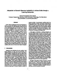
For the specific scenario where speed uniformly distributes over [0, vmax], PDF and CDF of the relative velocity along radius are illustrated in Figure 2. In this case, the relative velocity can be as large as 2vmax, where two nodes move oppositely.
Path Availability in Ad Hoc Network
5
1
CDF
PDF PDF, CDF
0.8 0.6 0.4 0.2
1
0 0
0.5
1 v vmax
1.5
2
Figure 2 PDF and CDF of relative velocity
As we can see from Figure 2, about 80% of the relative speed distributes within the range (0.3 ~ 1.3)vmax. This suggests us that very few nodes remain relative static and in general it is a little higher than one node’s. Although our analysis here is only specific to a certain mobility model, the methodology could still be applied to other models. 3.2
Link available time
Consider the one-hop link between two mobile nodes MN1 and MN2. Because of the centrosymetric nature of our model, without loss of generality we can assume that the initial distance between them is r, and the line connecting two points is parallel to X-axis. If we take MN1 as the reference point, then from the viewpoint of MN1, MN2 moves at a relative velocity vr whose distribution is described before, and MN1 remains static. After time t, MN2 moves out of the radio transmission range of MN1. The distance it traveled during this period is ρ. According to the law of cosine,
ρ (r, θ ) =
R 2 − r 2 sin 2 θ − r cos θ
(8)
The CDF of the link available time, i.e., the probability that the link available time is less than t is 2π
∞
0
vmin
Ft ( r , ψ , t ) = Ft ( r , 0, t ) =
∫ ∫ frv ( vr ,θ ) dv dθ
(9)
where vmin is the minimum required velocity to reach the border of the coverage area exactly after time t. v min ( r , θ , t ) =
ρ ( r ,θ ) t
The PDF of the link available time can be obtained from its CDF
(10)
6
Dan Yu, Hui Li and Ingo Gruber
MN2
ρ y
θ
R r
x
MN2
ψ MN1
Figure 3 Link available time
ft ( r , ψ , t ) =
∂Ft ( r ,ψ ,t ) ∂t
(11)
Now we could calculate the expectation of the available time for this wireless link ∞
E [ t r ,ψ ]( r , ψ ) =
∫ f t ( r ,ψ ,t )⋅t dt
(12)
0
Even more, we can conclude the mean link available time distribution between two arbitrarily chosen nodes, which is the mean value of link available time over all the possible position of MN2, i.e. ft ( t ) =
2π
R
0
0
∫ ∫ f t ( r ,ψ ,t )⋅r dr dψ
(13)
∞
∫
Ft ( t ) = f t ( t ) dt 0 t
=
2π R
∫ ∫ ∫ f t ( r ,ψ ,t )⋅r dr dψ
0 0 2π R
=
∫∫∫
0 0 2π R
=
0 t
(14) f t ( r ,ψ ,t )⋅r dr dψ
0
∫ ∫ Ft ( r ,ψ ,t )⋅r dr dψ 0
0
Therefore the average available time between two nodes is
Path Availability in Ad Hoc Network
E[t
7
2π ∞
(1)
( X )] =
∫ ∫ E [ tr(1,ψ) ( X )](r ,ψ )⋅r dr dψ
(15)
0 0
For the specific scenario where velocity uniformly distributes over [0, 1], the available time with different link length is illustrated in Figure 4. Several interesting things are noticed in the figure. First, in the beginning there are some flat regions (equal to zero) for r=0.0 or 0.7. This means that links are always available during this time, which can be explained by our “speed limit”. Because we have a maximum speed of vmax=1. If MN2 is inside the coverage of MN1, it cannot escape MN1’s coverage before a certain time. We call it “threshold time”, which is the minimum required time for MN2 to reach the coverage border of MN1, i.e. t th ( r , ψ , v max ) =
R −r vmax
(16)
Another thing to be noticed is the zero threshold time when MN2 stands at the border of radio coverage of MN1. At this point, availability immediately grows to 50% when MN1 start to move. From the microscope view, the border can be regarded as a line. Therefore MN2 has equal probabilities to move both into and out of MN1’s coverage. 1
CDF
0.8 0.6 0.4
r=0.0 r=0.7 r=1.0
0.2
0.5
1
1.5 t
2
2.5
3
Figure 4 Link available time CDF
Link availability at a given time t is the probability that a connected link at time 0 is still available at time t. This is the same as to say that it is the probability that a link is available after more than t seconds, which is Pa ( r , ψ , t ) = 1 − Fa ( r , ψ , t )
It is plotted in Figure 5.
(17)
8
Dan Yu, Hui Li and Ingo Gruber
0
Availability
0
1 0.8 0.6 0.4 0.2 0
0.2
0.5
0.4
1 vmax 1.5
0.6 r
0.8 2
1
Figure 5 Link availability as a function of link distance and time
3.3
Available time of multihop links (path)
Now we consider an end-to-end path with n (>=1) hops, which extends from mobile node MN1 along MN2, until it reaches MNn+1, and the length of each hop are r1, r2, … , rn. Obviously, these n hops are not totally independent of each other. For instance, the movement of intermediate node MN2 will affect both of its links to MN1 and MN3, Therefore there is dependencies between links from MN1 to MN2 and from MN2 to MN3 to are not entirely independent. However, to simplify our study, we may first neglect the effect of dependency between two consecutive links. Assume available time of each hop are random variables t1, t2, … , tn, whose distribution conforms to Figure 4. Then the link available time t of this n-hop link is a random variable that is the minimum value of the link available time of each of its n hops, t = min{ t1 , t 2 ,
1t
n
)
(18)
whose CDF is Ft
(n)
( t , r1 , r2 ,..., rn ) = P ( X ≤ t ) = 1 − P( X > t) n
=1−
∏ P ( X k >t )
=1−
∏ [1− P ( X k ≤t )]
=1−
∏ [1− Ft ( rk ,0,t )]
k =1 n k =1 n k =1
(19)
Path Availability in Ad Hoc Network
9
To get deeper insight into the available time of this n-hop path, we will concentrate our study on average path available time distribution. Follow the same derivation as (19), the CDF can be obtained with Ft
(n)
n
(t ) = 1 −
∏ [1− Ft (t )] = 1 − [1 − Ft (t )]
n
(20)
k =1
and the PDF is ft
(n)
(t ) =
∂Ft ( n ) ( t ) ∂t
= n[1 − Ft ( t )]
n −1
(21) ft ( t )
Now we can conclude average available time of the n-hop path as ∞
E[t
(n)
( X )] =
∫ f t( n ) ( t )⋅t dt
0 ∞
=
∫ n[1− Ft ( t )]n −1 f t (t )⋅t dt 0
(22)
∞
∫
= − t d[1− Ft ( t )]
n
0
∞
= lim t ⋅ [1 − Ft ( t )] t →∞
n
+
∫ [1− Ft (t )]n dt 0
1 0.8
CDF
0.6 0.4
n=1 n=2 n=4 n=8
0.2
0
0.5
1
1.5 t
2
2.5
3
Figure 6 Mean available time distributions in n-hop link
For the specific scenario that velocity is uniformly distributed between [0, 1] (unit/second), link available time distribution is illustrated in Figure 6. The average available time of the multihop path with different number of hops is revealed in Figure 7. The available time drops quickly from 2 for one-hop link to a little more than 0.5 for 3-hop link. However, the curve stays relative flat when we further
10
Dan Yu, Hui Li and Ingo Gruber
increase the number of hops in the path, which only drops from 0.45 for a 4-hop path to 0.24 for an 8-hop link. 2 1.75 Available time
1.5 1.25 1 0.75 0.5 0.25 2
3
4 5 Number of hops
6
7
8
Figure 7 Average available time in multihop path
For the average path availability in multihop cases, we have (n)
Pa
( t ) = 1 − Ft
(n)
( t ) = [1 − Ft ( t )]
n
(23)
In Figure 8 the link availabilities for the multihop link with different number of hops are given. The average available time can be obtained as (n)
E [ Pa
( t )] =
2π
R
0
0
∫ ∫ Pa( n ) ( t )t dt
(24)
1
n=1 n=2 n=4 n=8
Availability
0.8 0.6 0.4 0.2
0
0.5
1
1.5 t
2
2.5
3
Figure 8 Mean link availability versus time
It is obvious that the performance deteriorates very fast when number of hops increase. For instance, at time 1.3, on average half of the links will be invalid for single-hop link, whereas 0.7 for 2-hop links, 0.4 for 3 hop links and 0.2 for 8 hop links. This fast decrease of the availability strongly dissuades the usage of links with too many hops in ad hoc multihop routing algorithm.
Path Availability in Ad Hoc Network
4
11
Simulation
In order to verify our analysis and investigate the influence of our neglect of dependency between consecutive hops in a multihop link, we conducted simulations to measure the average available time. For each scenario, we generate n+1 nodes. Node k+1 (1≤ k ≤ n) is deployed uniformly inside node k’s radio coverage. Each node randomly chooses its direction and velocity from uniform distribution. The available time is measured when any node k+1 moves out of node k’s radio coverage. We randomly generate 1,000,000 such scenario and average over them. The parameters are summarized in Table 1. Table 1 Simulation parameters Parameter Radio transmission range R Speed distribution Direction distribution Position distribution
Value 1 Uniform [0, 1] Uniform [0, 2π] Uniform
We simulated the average path available time at different number of hops. They are plotted along with theoretical curve and relative error in Figure 9. As we can see, the simulation result is very near to the curve, with our theory slightly underestimates. The close-up observation unveils an interesting phenomenon. The relative error is almost invisible for single-hop links. However, the relative error reach its maximum value for 2-hop paths, and goes smaller with increasing number of hops. This can be explained by the dependency between consecutive hops of the multihop paths. Because the inter-hop dependency reduces the randomness between consecutive hops, if we take into account this dependency, the actual link available time performance should be a little better than our analysis. As there is no inter-hop dependency exists in a single-hop link, our simulation result should be very close to the theory (~0.5%). For a two-hop link, each hop has some dependency over the other. For a link with more hops, because each hop is only dependent to its immediate consecutive hops, but not the further hops, the effect of dependency in the whole link is averaged out. This explains the relative large error (~4.7%) for two-hop links in our prediction and it’s tendency of getting smaller with increasing number of hops. From the figure, we can easily convert it to real-world parameters. For example, if the radio transmission range is 100 meters, and maximum velocity is vmax=1 m/s, which simulates a pedestrian scenario. We can derive the average available time of a 3-hop link as 0.60 ⋅ 100 / 1 = 60 sec. This is far from enough for a normal human conversation. Therefore we either use more power to reduce the number of hops, or switch to other possibility such as a backup link with less number of hops.
12
Dan Yu, Hui Li and Ingo Gruber
2
0.05 Analysis Simulation Relative Error
0.045
1.6
0.04
1.4
0.035
1.2
0.03
1
0.025
0.8
0.02
0.6
0.015
0.4
0.01
0.2 0
Relative Error
Average available time
1.8
0.005
1
2
3
4 5 Number of hops in the link
6
7
0 8
Figure 9 Average available time in multihop link
5
Conclusions
In this paper we established a simple ad hoc network model. Based on the model, link and path availability properties in ad hoc networks are studied. Specifically, the available time and available probability in single-hop link and multihop path are carefully investigated. In a multihop path, impact of dependency between consecutive hops is also studied, which turn out to be negligible for general-purpose research. Our research of link availability can be regarded as groundwork for further analysis of ad hoc network performance, as well as a guide to ad hoc network routing protocol design, e.g. in optimization of route selection and route discovery algorithms.
References [1] MANET Working Group of IETF. http://www.ietf.org/html.charters/manetcharter.html [2] C. E. Perkins editor, “Ad hoc networking”, Addison - Wesley, 2000 [3] A Bruce McDonald and T. F. Znabi, “A path availability model for wireless ad hoc networks”, Proc. IEEE WCNC, New Orlean, USA, Sept. 1999 [4] Elizabeth M. Royer, "Routing in Ad hoc Mobile Networks: On-Demand and Hierarchical Strategies", http://www.cs.ucsb.edu/~eroyer/publications.html