Pattern Based Iterative Method for Extreme Large Power/Ground ...

> REPLACE THIS LINE WITH YOUR PAPER IDENTIFICATION NUMBER (DOUBLE-CLICK HERE TO EDIT)
REPLACE THIS LINE WITH YOUR PAPER IDENTIFICATION NUMBER (DOUBLE-CLICK HERE TO EDIT) < commercial boundary element method (BEM) based tool. Here, typical metal slice resistance stands for the mean values of all the extracted resistors in a certain layer. Column „typical via resistance‟ in layer M1 means the resistance of vias between M1 and M2, and so on. For M2-M4 layers, node number stands for the number of vias connected to the underlaid layer. While in layer M1, it stands for the number of pins of different gates connected to the p/g grids. From Table I, we can see that, in M1, the typical via resistance is about 1/5 of the typical metal slice resistance. Also, due to the increased rail width in M2 and M3, the typical metal slice resistance in the two layers is low. Thus, in layer M1, if the branch current on a given via is the same as that on a metal slice, the voltage drop on that via is also about 1/5 of that on the metal slice. However, in layer M1, this is not the case, because the number of vias is less than the number of pins of different gates. Note that in Table I, the node ratio of M1 to M2 is about 35, which means that on average, currents from 35 gates will flow through one via between M1 and M2. This configuration will cause the voltage drop on the vias to be amplified by the ratio of larger branch currents and the currents on the metal slices. As a result, even if the resistance of some via is just 15% of that of a metal slice in layer M1, the voltage drop on a via (M1-M2) can be 6 times of that on a metal slice. Even worse, if the current is not be distributed evenly, the voltage drop on some vias can be much larger. For M2, M3 as well as upper layers, due to the decreasing resistance of the metal slices, even if the branch current is the same, the voltage drop on a via will have the same magnitude comparing with that on a metal slice. In addition, the situation discussed above is a process independent problem. Even if the process parameters remain the same, when designing a denser p/g grid, the length of metal slices will become shorter. Hence, the resistance of the metal slices will become smaller, while via resistance remains the same under certain processes. In summary, in order to maintain the accuracy, we have to model vias explicitly even in early stage simulation. Figure 4 shows our resistive 3D p/g grid model with via resistance. From this figure, we can see that when the via is modeled explicitly, the topology of the p/g grid modeled in 3D is different than that of a 2D grid. The connection degree of each node in x-y plane is reduced from 4 to 2. Later, we can see that this property is very useful in matrix generation.

3

III. INTRODUCTION OF PREVIOUS METHODS A. Linear System Generation To build circuit equations by using the extracted resistance of metal slices and vias, nodal analysis (NA) method is usually used [5], which is based on Kirchhoff‟s voltage and current rules. Analyzing the matrix construction process carefully, we will find that each metal slice is mapped into a resistor first. Then, according to a certain strategy, all the terms of resistors are given unique node sequential numbers. After that, a resistor from node a to node b can be stamped into four elements in the simulation matrix, as shown in Figure 5. When all the resistors have been mapped, we can get the complete simulation matrix, which is a symmetry positive definite (s.p.d.) matrix.

Fig. 5. Fill in mode of a resistor under NA method B. Linear System Solver The matrices generated by NA method are large sparse matrices. Many previous works try to find efficient method to solve this kind of large linear systems. Generally speaking, these methods can be classified into three categories: direct method, iterative method and random method. The LU decomposition method [10] is a well-known direct method, while preconditioned conjugate gradient (PCG) [5], alternative-direction-implicit (ADI), [4] and multi-grid (MD) [2] methods are typical iterative methods. Methods of the first two categories try to solve the generated linear system Ax = b in an exact way. However, methods of the third category try to solve the linear system in a stochastic, an approximate way stochastically, which are based on random experiments. The typical method in this category is random-walk (RW) approach [3]. Actually, it is difficult to say which method is more efficient in general, even if the implementation issues are not considered. Each of them explores some special characteristics of the p/g grid simulation problem and accelerates the simulation process in different ways. Table II summarizes the reported performance of some methods. TABLE II REPORTED PERFORMANCE OF DIFFERENT LINEAR SOLVERS FOR DC SIMULATION Maximal Run CPU Name Reported Mem Ref Time Type Size LU 0.6 M 1114.1 400Mhz NR [2] PCG 5.1 M 1181.6 666Mhz NR [5] MG 0.6 M 69.2 400Mhz NR [2] RW 2.7 M 1500 2.8 Ghz 300 Mb [3] a Column Run Time has the unit of second

Fig. 4. 3D P/G grid model with vias

From Table II, we can see that all these methods can handle

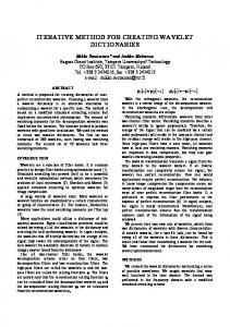
> REPLACE THIS LINE WITH YOUR PAPER IDENTIFICATION NUMBER (DOUBLE-CLICK HERE TO EDIT) < large size grid circuits within half an hour. However, when the matrix size increases, all of them will suffer from the large memory cost. When a p/g grid is excessive large, even loading the design from database to memory becomes very difficult. Also, it is impossible to build the simulation matrix or allocate memory for auxiliary working structures, especially on a 32-bits system. This is the main reason why hierarchical method is widely used in practical p/g grid simulation. Although the increase in both die size and integration density is the main reason for large memory usage of the p/g grid simulation, lack of awareness about the regular structure of a p/g grid also contributes to excessive memory uses. We have analyzed the resistance data, extracted from M1 in a CPU benchmark by using a BEM solver. We find that although many metal slices are extracted from M1, they only have few different kinds of values. Figure 6 shows the resistance data distribution of the layer M1.

Fig. 6 Resistance distribution in M1

inner geometry structure of p/g grids of each block would be similar to one another. In this paper, we call this similarity of inner geometry structure of different blocks in a die the global patterns. Global patterns exist because the p/g grid is a special net routed in global area. It is always designed to be a regular one in early design stage, which means that in a certain metal layer, each rail has the same width and the pitch between two rails is also identical. Further, because the vias can only be laid down at the places that the upper metal rails intersect with the lower rails, the evenly distributed metal rails will cause evenly distribution of vias. Figure 7 shows a uniform partition scheme, where adjacent blocks overlap with each other. From this figure, we can see that since blocks have the same size, the inner p/g grid structures (including the number of rails and the number of metal slices in a rail) are completely identical in geometry, no matter where two blocks are located. B. Local Pattern However, the property of partial-similarity not only exists in global areas, it also exists in local areas. Figure 8 shows an irregular partition scheme where blocks are different in size. The block located in the left corner contains two metal rails routed in a vertical metal layer. The details of these two rails look much alike as shown in Figure 2. Then, from Figure 2 we can see that, even in the local area, different rails are similar to one another. In this paper, we call this kind of similarity local patterns. Further if the vias are evenly distributed, then different metal slices are identical. This kind of similarity in a rail is called hyperfine local patterns.

From this figure, we can see that only 7% resistors extracted from M1 have different values out of the listed four values, and 70% resistors have their values equal to 0.01 ohm. The reason is that the p/g grids are usually very regular in geometry. Also, due to the evenly distribution of vias in each metal layer, the shapes of most metal slices are similar to each other and their resistances are almost the same. Due to the fact that the number of the resistors extracted from M1 is very large, if we know the geometry information in advance, we can save a lot of time and memory even in the early extraction process. IV. P/G GRID PATTERNS As mentioned in the Section III, the previous simulation methods do not fully explore the geometry properties of p/g grids. In the following, we will first explain the pattern concept in p/g grids. Then we show that when pattern structures are used in extraction, due to the special stamps in the simulation matrices, the computation complexity and the memory usage can be reduced dramatically. A. Global Pattern The most important geometry property of regular p/g grid is its natural partial-similar property, which means that if we partition a complete regular p/g grid into smaller blocks in x-y plane, such that the shape of different blocks is similar, the

4

Fig. 7. The x-y plane partition with regular overlapped blocks

Fig. 8. The x-y plane partition with irregular separated blocks

> REPLACE THIS LINE WITH YOUR PAPER IDENTIFICATION NUMBER (DOUBLE-CLICK HERE TO EDIT) < V. PATTERN BASED SIMULATION ALGORITHM A. Overall Algorithm After different kinds of pattern structures are defined, we can introduce our pattern based simulation algorithm. This algorithm has 5 main steps, which are shown in Figure 9. The details of this algorithm will be explained in the following sub-sections.

5

and build a smaller linear system equation Ax=b. In this way, when we want to know the voltage distribution in other blocks, we just need to replace the current distribution of the previous pattern block with the new one and solve the linear system again. Another partitioning strategy is to divide the whole p/g grids according to logical blocks, especially considering the embedded IP blocks. This strategy will generate sub-blocks as shown in Figure 8. In this case, if the p/g grids are also under C4 bumps, the block boundary has to be aligned to the C4 bumps. In addition, because different logic blocks usually have different size, the user may define a threshold to identify blocks within a certain geometry variations and consider them as the same pattern. The complete partition strategies used in our algorithm is given in Figure 10. Read p/g grid information and block information

Fig. 9. The main steps in pattern based simulation algorithm In this algorithm, when a p/g grid is given, it first identifies the global patterns, which are all the blocks that are approximate in geometry size. In practical design, there usually have a lot of identical function blocks, i.e., in a multi-core microprocessor, there are a couple of ALU Units, Floating Points Process Units, Register Files, and so on. All these blocks can be treated as global patterns, such that one extracted block can represent the other one in geometry. Also, the user can define a strategy to identify the similarity of global patterns. In this case, even if two blocks are not exactly identical, but are similar, we still can treat them as the same (global patterns). Thus, when the first step has been finished, we can reduce global blocks to essential one with different sizes. Then, we can further identify the local patterns in the reduced global blocks. This step will merge all the rails that are similar in geometry to a certain rail to form another essential rail set. Also, there is a regularization process, which may handle the p/g grids that are relatively irregular in rail size. After the regularization process, a regular grid can be generated that the pattern-based extraction process is then used to translate local patterns into sub-matrix structures, which are the essential part of the simulation matrix. These sub-matrices will be used as the input parameters of pattern-based PCG solver. Finally, after the PCG process is finished, we can get the voltage distribution of all the nodes.

B. Partitioning Strategy In order to identify all the global patterns, we have to first choose a partitioning strategy. There are at least two kinds of partitioning strategies. For example, if the p/g grids are under a C4 package, we can partition the whole grid into sub-blocks along with the C4 bumps (or C4 pads, a special structure to provide power connection in Flip Chips) [8]. This strategy will generate identical sub-blocks, as shown in Figure 7, which does not consider what real logical elements are packed in the sub-blocks. This kind of partitioning will generate only one global pattern. Also, due to the good locality property [8] (local current variations only affects local voltage variations), we only need to extract the p/g grids in one global pattern of sub-blocks,

Choose Partition Strategy

C4 bump based

Logical based

Define a proper size of basic block considering real size of blocks then partition the grid

Merge the same size logical blocks into a pattern category

If possible, align blocks to C4 bumps

Fig. 10. The partitioning flow to determine global pattern In general, if a design has lots of identical logical blocks, each of which has different style P/G grid design, it is better to do partition according to logical blocks other than C4 blocks. This is because different logical blocks tend to have different local patterns. If we do partition based on the sub area defined by C4 bumps, we may destroy lots of local patterns and cause difficulty in local pattern extraction process. Further, if the quality of local pattern is not good enough, the overall efficiency of the pattern based simulation process will be less obviously. C. Regular Grid Extraction In each global pattern block, if the p/g grid is a regular grid, we can identify the local pattern easily, because all the geometry information is defined by the grid geometry parameter.

> REPLACE THIS LINE WITH YOUR PAPER IDENTIFICATION NUMBER (DOUBLE-CLICK HERE TO EDIT) < Table III gives a practical grid parameters used in a microprocessor. Firstly, by using these parameters, we determine the number of rails and then the coordinates of each rail for the given layer within a global pattern block. TABLE III P/G GRID GEOMETRY PARAMETER Layer

Width

Pitch

Square Resistance

M1 0.48 3.2 9.0e-2 M2 0.48 3.2 9.0e-2 M3 0.8 4.5 9.0e-2 M4 0.6 3.2 7.1e-2 M5 1.2 5.3 5.5e-2 M6 2.52 8.6 3.7e-2 M7 26 122 2.2e-2 a Column Width and Pitch shares the unit of um a Column Square resistance shares the unit of Ohm

Secondly, by combing the rail coordinates in the upper layer against the ones in lower layer, we may get the coordinates of intersection point (or called “via coordinates”). These intersection points divide each rail of the medium layer into metal slices.

6

Thus, once we know this coordinates, we can get the length of each metal slice, as well as the number of metal slices in a rail. Due to the regular distribution of the metal rails and vias in each layer, we only need to extract and store the geometry information of one typical metal rail, which is named Then, in the next step, we can translate the pattern rail structure into the sub-matrix structure and perform our simulation based on these pattern structures. Figure 11 a local pattern rail. shows our regular grid extraction algorithm. D. Sub-Matrix Generation We notice that the position of elements stamped into the matrix is highly correlated to the given node sequence. Also, the difference in node sequence between two terms of a resistor controls the spacing between two stamp-in elements. Thus, assuming the node sequences of a resistor are not consecutive from the left term to the right term, the stamp-in elements (usually four) generated by this resistor are separated from one another. Under this condition, the shape of the generated sub-matrix will become relatively banded for certain metal rail. In order to translate the local pattern into a regular sub-matrix form with the smallest band, we have to let the node number increase one by one along with the routing direction of the metal rails consecutively. In this way, we can translate the local pattern into a tri-diagonal sub-matrix as show in Figure 12.

Fig. 12. Stamps of rails using our node order

Fig. 11 Extraction algorithm for regular grid

Due to the local similarity, rails are identical in a local area for regular p/g grids. Therefore, after the simulation matrix is constructed, we can get many identical tri-diagonal sub-matrices in the diagonal block of the simulation matrix. Obviously, there is no need to store all the tri-diagonal matrices in the memory, and one is good enough for a local block. Furthermore, if the global grid is partitioned using C4 based strategy mentioned in Figure 10 (more details can be found in [8]), storing one tri-diagonal matrix in each layer is enough for the whole p/g grid because all the blocks share the same size. Particularly, for a special p/g grid in which “hyperfine local patterns” exist, it is even not necessary to store each tri-diagonal matrix. The reason is due to the following regular structure of the tri-diagonal sub-matrix t in the simulation matrix, which can be obtained by using the previous introduced stamp-in strategy:

> REPLACE THIS LINE WITH YOUR PAPER IDENTIFICATION NUMBER (DOUBLE-CLICK HERE TO EDIT) < 2 g  v i  j  tij    g j  i  1 or j  i  1 i 1,i  n 0 other  t11  tnn  g  v t12  tn ( n 1)   g

7

(3)

Here, g is the conductance of a metal slice in the rail; v is the conductance of a given via in this rail; n is the number of metal slices in the rail. Obviously, based on this structure, only the numbers g, v and n have to be stored for the local p/g grid. Another advantage of using this node sequence is that the sub-matrix generated by conductance of vias can also be regularized. Figure 13 shows a typical structure of such a sub-matrix.

Fig. 14. The structure of the simulation matrix

Fig. 13. Sub matrix of vias Because vias in two adjacent layers share the same resistance, the sub-matrix p generated by vias has the following regular structure, as shown in (4), where α andβ are two integers equal to the via number per rail in two adjacent layers, while k1 and k2 are integers ranging from 1 toα and 1 toβ .   i   1    k1     g v if           (4) pij    j    1   k2     0 other  A typical simulation matrix generated by using our translation method is shown in Figure 14. (Note that this figure is not drawn to scale, because M1 and M2 always contains nodes magnitude different with other layers, if draw to scale we can not see the structure clearly.) From this figure, we can see clearly that, by using this node sequence, we can translate the geometry patterns into matrix patterns successfully. Notice that the power grid matrix is similar to the ground grid matrix and there are a lot of identical tri-diagonal matrices and regular via matrices in the circuit matrix. Thus, by storing key sub-matrices in the simulation matrix, the memory usage can be reduced dramatically.

Second, in certain layer, within a block boundary, it calculates the resistance of all the metal slices and the mean value of them. Also, if the width of each metal slices are different, the mean value of width parameter has to be calculated. Third, the mean resistance is transformed into a standard geometry shape reversely using the mean value of width parameter and the sheet resistance parameter in this area. Fourth, it replaces all the metal slices in the original layout by the standard metal slices, which will make an irregular grid to become a regular one. Figure 15 shows a simulation matrix extracted from the p/g grid of an industrial CPU case by using our regularization scheme. From this figure, we can see that after regularization, there are still lots of patterns in layer M1and M2.

Fig. 15. A regularized simulation matrix with vias

E. Irregular Grids For most cases in industry, especially in later design stages, the p/g grid is not as regular as that in early design stage. Designers always make tiny changes anywhere they think suitable to fix power supply problems. In order to handle irregular grids, we can use a regularization process. First, this process identifies all the metal slices using the layout information to calculate coordinate. It is similar to the algorithm introduced in Figure11.

Also, Table IV shows the simulation result of 3 test p/g grids before and after regularization process. From the table, we can see that the regularization process affects the simulation result with inaccuracy of less than 5% of errors. The reason is that in the industrial p/g grids, it tends to use a very dense mesh in M1 and M2, while using relative sparse mesh with larger metal width in M3-M7.

> REPLACE THIS LINE WITH YOUR PAPER IDENTIFICATION NUMBER (DOUBLE-CLICK HERE TO EDIT) < TABLE IV WORST VOLTAGE DROP VARIARATION Grid Name

Matrix Size

Power

Before Reg

After Reg

Var Ratio

TG1 10k 20 208.7 199.3 -4.5% TG2 25k 33 39.5 40.8 3.3% TG3 36k 45 154.3 147.5 -4.4% a Column Power has the unit W a Column Before Reg and After Reg have the unit mv a Column Before Reg stands for the worst voltage drop variation before regularization and After Reg stands for the worst voltage drop after regulariztion

Further, changes in later design stages always happen in M3-M7, because M1 and M2 are too crowded to make any changes. Since in the simulation matrix, only less than 10% stamp-in elements are extracted from M3-M7, the changes in geometry does not affect the generated matrix significantly. Also, designers can control the simulation accuracy by adjusting the index factor in regularization process. The index factor, which is a real number ranging from 0 to 1, will affect the local pattern extraction process. If the index factor is set to a lower value, the local pattern extraction process will extract fewer patterns. Otherwise, the local pattern extraction process will identify more patterns. When the index factor is set to 1, all rails will be extracted. Thus the pattern information will be ignored. In this case, we will simulate the original irregular gird. Although no accuracy will be sacrificed, the memory cost will increase dramatically. F. Accuracy Improvement by Global Iterations After finishing the local block simulation, we may get the voltage distribution result. However, because the global blocks are mutually correlated, and the current distribution is usually not uniform, thus if we set a strict accuracy threshold, we may find that the errors may fail to meet accuracy requirement. Therefore, in order to get more accurate simulation results, we have to perform a global-like iteration process to improve the accuracy. This process is especially needed when the design is a wire-bond based p/g grid. It is because for C4 based design, the C4 bumps can exist in the center of the die. Thus, the dense vias help to conduct the currents from C4 bumps to the bottom layers immediately without diffusing in the x-y plane. This is demonstrated clearly by the current contour map in [8] and also implies that large current is less likely to flows across the block boundary. Therefore by using the partition strategy mentioned previously, the errors caused by initializing all the boundary currents to zero are not significant. According to our experiments, if the locality property is strong, the error is small even if the current is magnitude different inside different blocks. We found that about less than 5 times global iterations can be sufficient reduce the maximal analysis error to uV magnitude. However, for wire-bond designs, power pads are only seated at the die boundary and large current may flows across the block boundary to relay power. Therefore initializing the boundary current to zero will cause larger errors. In order to control this kind of errors, we use accuracy improvement process shown in Figure 16. Here, an important point is that we do not need to generate the global matrix to perform the global iteration process. Also, this strategy can

8

reach the global convergence, as it can be proved that it equals to a Jacobi-like iteration process. The proof sketch is given below: First, if we construct the global simulation matrix using the same node numbering strategy and stamping strategy as in local matrices generation, we will find that the global matrix has the form similar to figure 14. Therefore, we still can use a block tri-diagonal matrix to represent it. Equation (5) shows a simplified global matrix containing three metal layers.

 A G   DT 

D B E

T

 E  C 

(5)

Fig. 16. global iteration accuracy improvement process Second, although after partition, the local simulation matrices of partitioned blocks are completely different from the tri-diagonal sub-matrices A, B, and C in the global G matrix, they are still similar to matrix G in structure. If we delete boundary rows and columns, only leave the rows and columns related to local nodes set, we would get the local simulation matrices. Because the deleting process does not change the values of elements in diagonal blocks, the remaining local simulation matrices are still diagonal dominant. Thus, the global matrix can be treated as the combination of all local matrices after a reordering process. Third, once a local system is solved, we can get the voltages of local nodes distributed in different layers simultaneously. Also, because all the boundary currents between adjacent blocks are set to zero, after finishing solving all local blocks, we can get all the node voltages. Then by updating the node

> REPLACE THIS LINE WITH YOUR PAPER IDENTIFICATION NUMBER (DOUBLE-CLICK HERE TO EDIT) < voltage, we can recalculate the boundary currents. Due to the equivalence of local matrices and the global matrix, this iterative process can be treated as the relaxation process in Jacobi updating applied to the global matrix. Also, because the global matrix is an s.p.d matrix, this iteration process will converge definitely. Also, for wire-bond designs, special techniques must be used. Because the pads only exist at the die boundary, we have to set all the voltage of via node at top layer to Vcc at the beginning. Otherwise none of the partition strategy will work due to lacking of pads. Then, when the first solving is finished, we can calculate the current on the top layer vias. This current information can be used to recalculate the voltage distribution at the top layer, and then the next iteration can begin. Generally speaking, the convergence ratio depends on two aspects. The most important one is still the via density, because it controls the current diffusing ratio at the middle and bottom layers. The top layer metal width is another factor. Although the large current will flow across the block boundary, due to the wide and thick metal rails are always used in practical designs, the voltage differences will be small at top layer. So, the initial setting of Vcc is reasonable. Also, the iteration on current other than the voltage at the top layer can also help the converge ratio. Of course, because this method is not a general method, when a wire-bond design has poor locality property and the top layer metal rails are also very thin, the convergence speed will be slow too.

VI. NEW PRE-CONDITIONER A. Drawbacks of the Traditional Preconditioner In order to solve the generated local linear system, efficient inner solver has to be developed. According to our experimental results, the PCG method will be faster than the LU method when the iteration times are low. On the other hand, the most effective way to improve the convergence speed of the iterative method is to use a good preconditioner [10]. However, the general preconditioner, such as Incomplete LU decomposition (ILU) and Incomplete Cholesky decomposition (ICD) may not take full advantage of the pattern structures of a p/g grid. This will lead to the low memory efficiency of these preconditioners. Also, the traditional preconditioner handles all the matrices in the same way, so that they cannot benefit from the special structures of the original matrix. Thus, the only way to accelerate these preconditioners is to choose a relatively small drop-threshold. However, small drop-threshold will lead to larger fill-in to the original matrix. TABLE V TYPICAL FILL IN FACTOR VS. DROP THRESHOLD Drop off threshold

Fill in factor

Iteration times

1e-1 1.5 1e-2 2.79 1e-3 10.96 1e-4 48.41 a PCG method is used for Iteration a Basic precondition method is ILUT [10] a The stop error tolerance is set to 1e-6

221 93 44 17

9

Table V shows typical fill-in factors (the number of nonzero elements in precondition matrix to that of the original matrix) under different kinds of drop-threshold for a test circuit matrix. From this table, we can see that using this method to accelerate the p/g grid simulation is unreasonable due to the extensive memory usage. B. Construction of the New Preconditioner In order to overcome the drawbacks of the general preconditioner, a new preconditioner is proposed to fully explore the pattern structures of p/g grids. As mentioned above, the most efficient way to accelerate the performance of traditional preconditioners is to introduce more fill-in elements. However, if the fill-in factor is as large as that in LU decomposition process, the iteration process loses all its advantages. Thus, how to improve the performance of preconditioner with less memory is one of the main contributions of this paper. In this section, we begin to reconstruct a new preconditioner based on the inverse matrix with approximation. As we know, the inverse of simulation matrix is an ideal preconditioner, but the computation cost of the inverse is unreasonably high, while the memory cost of it equals to that of the LU decomposition. However, some special matrices are exceptions for this rule, for instance, the tri-diagonal matrix. The inverse of a tri-diagonal matrix is easy to obtain by using LU decomposition process. More importantly, no fill-in elements will be introduced during this decomposition process. Remember that under our node sequence, local patterns can be translated into identical tri-diagonal matrices. Thus, if we can exploit the inverse of tri-diagonal matrices to construct the approximate inverse of the original matrix, the performance can therefore be improved. For simplification, we take the circuit matrix of a two-layer regular p/g grid as an example. The structure of the circuit matrix is shown in (6).

A C T 

C B 

a  A      a 

b  B     (6)  b 

Here, A and B are tri-diagonal matrices which consist of small tri-diagonal matrixes a and b (sub-matrix generated by local rail patterns). Sub-matrix C is generated because of vias. For this structured sparse matrix, we can perform Schur-like decomposition as shown in (7).

A C T 

C  I  B  C T A1

 A  I    I  B ' 

A1C   (7) I 

In formula (7), the original matrix is decomposed into the product of three matrices. Among the 3 matrices, the left one and the right one are basic elimination matrices, while the middle matrix is a block diagonal matrix. Here B’ is a new matrix given in (8)

B '  B  CT A1C (8) Because the three matrices are easy to inverse, the ideal inverse of original matrix can be represented as (9)

> REPLACE THIS LINE WITH YOUR PAPER IDENTIFICATION NUMBER (DOUBLE-CLICK HERE TO EDIT)
REPLACE THIS LINE WITH YOUR PAPER IDENTIFICATION NUMBER (DOUBLE-CLICK HERE TO EDIT)
REPLACE THIS LINE WITH YOUR PAPER IDENTIFICATION NUMBER (DOUBLE-CLICK HERE TO EDIT) < He gave many insightful suggestions during the course of this work. We also thank the reviewers for their constructive comments, which significantly improve the presentation of this paper. REFERENCES [1] [2]

http://www.itrs.net/Common/2004Update/2004Update.htm J. N. Kozhaya, S. R. Nassif and F.N. Najm: "A multigrid-like technique for power grid analysis", IEEE Trans. Computer-Aided Design, vol.21, no.10, Oct. 2002, 1148-1160 [3] H. Qian, S. R. Nassif, S. S. Sapatnekar: "Power Grid Analysis Using Random Walks", IEEE Trans. On Computer Aided Design, Volume 24, Issue 8, Aug. 2005 Page(s):1204 - 1224 [4] W. Guo, S. X. D. Tan, "Circuit level alternation-direction-implicit approach to transient analysis of power distribution networks", International Conference on ASIC Proceedings, 2003, Beijing, 246-249 [5] T. Chen and C. C. Chen: "Efficient large-scale power grid analysis based on preconditioned Krylov-subspace iterative methods", DAC2001 Proceedings, pp. 559-562 [6] J. M. Wang and T. V. Nguyen, "Expended Krylov Subspace method for reduced order analysis of linear circuits with multiple sources", In Proceeding of IEEE/ACM Design Automation Conference, pp. 247-252, Los Angeles, Jun. 2000. [7] M. Zhao, R. V. Panda, S. S. Sapatnekar and D. Blaauw, "Hierarchical analysis of power distribution networks", IEEE Trans. On Computer Aided Design, vol. 21, no. 2, pp. 159-168, Feb. 2002. [8] E. Chiprout, "Fast flip-chip power grid analysis via locality and grid shells", ICCAD 2004 Proceeding, pp 485-488 [9] Chung-Kuan Cheng, John Lillis , Shen Lin, Norman Chang, "Interconnect Analysis and Synthesis", Awiley-Interscience Publication, 2000 [10] Saad, Yousef, Iterative Methods for Sparse Linear Systems, PWS Publishing Company, 1996. [11] Y. Cai, Z. Pan, X. Hong, S.X.-D. Tan et al, “Relaxed hierarchical power/ground grid analysis”, ASPDAC 2005 Proceeding, pp 1090-1093 [12] J. Shi, Y. Cai, S.X.-D. Tan, X.Hong, “High Accurate Pattern Based Precondition Method for Extremely Large Power/Ground Grid Analysis”, ISPD 2006 Proceeding, pp 108-113

Jin Shi received his B.S degree in Computer Science & Technology from University of Electronic and Science and Technology of China (UESTC) in 2003. Now, he is studying for PhD Degree in Tsinghua University and doing researches in EDA Lab. His research interests include Power/Ground network analysis and optimization techniques. Yici Cai (M‟04) received her B.S degree in Electronic Engineering from Tsinghua University in 1983 and her M.S degree in Computer Science & Technology from Tsinghua University in 1986. She has been a professor in the Department of Computer Science & Technology, Tsinghua University. Her research interests include physical design automation for VLSI integrated circuits algorithms and theory, power/ground distribution network design and optimization, high performance clock network design and routing, low power physical design. Jeffrey Fan received his Bachelor of Science degree in electronics engineering from National Chiao Tung University, Taiwan, R.O.C., and Master of Science degree in electrical engineering from State University of New York, Buffalo, in 1983 and 1987, respectively. He is currently a PhD candidate in electrical engineering at the University of California, Riverside. From 1988 to 2002, he held various senior technical positions at Western Digital, Emulex Corporation, Adaptec Inc., and Toshiba America. He served as Vice President of Vivavr Technology, Inc., and General Manager/Co-Founder of Musica Technologies, Inc. His research interests include very large scale integration simulation, modeling, and power grid optimization. Sheldon X.-D. Tan (S'96-M'99-SM‟06) received his B.S. and M.S. degrees in electrical engineering from Fudan University, Shanghai, China in 1992 and

13

1995, respectively and the Ph.D. degree in electrical and computer engineering from the University of Iowa, Iowa City, in 1999. He is an Associate Professor in the Department of Electrical Engineering, University of California, Riverside. He was a faculty member in the Electrical Engineering Department of Fudan University from 1995 to 1996. He worked for Monterey Design Systems Inc. CA, from 1999 to 2001 and Altera Corporation CA, from 2001 to 2002. His research interests include several aspects of design automation for VLSI integrated circuits – modeling and simulation of analog/RF/mixed-signal VLSI circuits, high performance power and clock distribution network simulation and design, signal integrity, power modeling, thermal modeling, thermal optimization in VLSI physical and architecture levels and embedded system designs based on FPGA platforms. Dr. Tan is the recipient of NSF CAREER Award in 2004. He also received the UC Regent's Faculty Fellowship in 2004, 2006. Dr. Tan received a Best Paper Award Nomination from 2005 IEEE/ACM Design Automation Conference, Best Paper Award from 1999 IEEE/ACM Design Automation Conference. He also co-authored book "Symbolic Analysis and Reduction of VLSI Circuits" by Springer/Kluwer 2005 and Advanced Model Order Reduction Techniques for VLSI Designs, by Cambridge University Press 2007. He is an associate editor for Journal of VLSI Design and served as a technical program committee member for ASPDAC, BMAS, ASPDAC, ISQED, ICCAD. Xianglong Hong (F‟2004) graduated from Tsinghua University, Beijing, China in 1964. Since 1988, he has been a professor in the Department of Computer Science & Technology, Tsinghua University. His research interests include VLSI layout algorithms and DA systems. He is the fellow of IEEE and the Senior Member Chinese Institute of Electronics.