Pattern Recognition and Machine Learning Techniques for Algorithmic Trading
Corvin Idler 20, Rue de la Poste, L-2346 Luxembourg
[email protected]; Mat.Nr.: 7529953
M A S T E R’ S T H E S I S
submitted in partial fulfillment of the requirements for the degree of Master of Science in Business Administration and Economics
Supervisor:
Dipl. Ök. B.Sc. Dominik Ballreich
Assessor:
Prof. Dr. Hermann Singer
completion time:
6 months as part-time student
submitted on:
21st July, 2014
Verfahren der Mustererkennung und des maschinellen Lernens für algorithmisches Handeln
Corvin Idler 20, Rue de la Poste, L-2346 Luxembourg
[email protected]; Mat.Nr.: 7529953
MASTERARBEIT
zur Erlangung des Grades eines Master of Science (M. Sc.) Wirtschaftswissenschaft –Magister der Wissenschaft–
Betreuer:
Dipl. Ök. B.Sc. Dominik Ballreich
Prüfer:
Prof. Dr. Hermann Singer
Bearbeitungszeit:
6 Monate als Teilzeitstudierender
eingereicht am:
21. Juli 2014
© Copyright 2014 Corvin Idler 20, Rue de la Poste, L-2346 Luxembourg
[email protected]; Mat.Nr.: 7529953
All Rights Reserved
ii
Declaration I hereby declare and confirm that this thesis is entirely the result of my own original work. Where other sources of information have been used, they have been indicated as such and properly acknowledged. I further declare that this or similar work has not been submitted for credit elsewhere. I give my written consent to this work being tested for plagiarism by means of automated detection services. Luxembourg, 21st July, 2014
Signature:
Erklärung Hiermit versichere ich an Eides statt, dass ich die Masterarbeit selbständig und ohne Inanspruchnahme fremder Hilfe angefertigt habe. Ich habe dabei nur die angegebenen Quellen und Hilfsmittel verwendet und die aus diesen wörtlich oder inhaltlich entnommenen Stellen als solche kenntlich gemacht. Die Arbeit hat in gleicher oder ähnlicher Form noch keiner anderen Prüfungsbehörde vorgelegen. Ich erkläre mich damit einverstanden, dass die Arbeit mit Hilfe eines Plagiatserkennungsdienstes auf enthaltene Plagiate überprüft wird. Luxemburg, den 21. Juli 2014 Unterschrift:
iii
Contents Declaration
iii
Abstract
ix
1 Introduction
1
1.1
Motivation, background and rationale . . . . . . . . . . . . . . . . . . . . . . . . . . .
1
1.2
Literature survey and research gap . . . . . . . . . . . . . . . . . . . . . . . . . . . . .
2
1.3
Research hypothesis and contribution . . . . . . . . . . . . . . . . . . . . . . . . . . .
4
1.4
Stucture . . . . . . . . . . . . . . . . . . . . . . . . . . . . . . . . . . . . . . . . . . . .
5
2 Efficient Market Hypothesis – Meta-Perspective & Academic Context
6
2.1
History . . . . . . . . . . . . . . . . . . . . . . . . . . . . . . . . . . . . . . . . . . . .
6
2.2
Definition . . . . . . . . . . . . . . . . . . . . . . . . . . . . . . . . . . . . . . . . . . .
6
2.3
Paradoxicality . . . . . . . . . . . . . . . . . . . . . . . . . . . . . . . . . . . . . . . . .
7
2.4
Validity . . . . . . . . . . . . . . . . . . . . . . . . . . . . . . . . . . . . . . . . . . . .
7
2.5
Self-destructibility of predictability . . . . . . . . . . . . . . . . . . . . . . . . . . . . .
11
2.6
Conclusion – Intellectual reconciliation . . . . . . . . . . . . . . . . . . . . . . . . . . .
11
3 Machine Learning – Conceptual & Theoretical Framework
14
3.1
Definition . . . . . . . . . . . . . . . . . . . . . . . . . . . . . . . . . . . . . . . . . . .
14
3.2
Learning paradigms . . . . . . . . . . . . . . . . . . . . . . . . . . . . . . . . . . . . .
14
3.3
Mathematical model and notation . . . . . . . . . . . . . . . . . . . . . . . . . . . . .
16
3.4
Supervised learning process . . . . . . . . . . . . . . . . . . . . . . . . . . . . . . . . .
18
3.4.1
Identification of required data . . . . . . . . . . . . . . . . . . . . . . . . . . . .
18
3.4.2
Data pre-processing . . . . . . . . . . . . . . . . . . . . . . . . . . . . . . . . .
26
3.4.3
Definition of training set (Feature selection) . . . . . . . . . . . . . . . . . . . .
28
3.4.4
Definition of training set (Sample selection) . . . . . . . . . . . . . . . . . . . .
34
3.4.5
Algorithm selection . . . . . . . . . . . . . . . . . . . . . . . . . . . . . . . . . .
35
3.4.6
Training & Parameter tuning . . . . . . . . . . . . . . . . . . . . . . . . . . . .
37
3.4.7
Evaluation with test set . . . . . . . . . . . . . . . . . . . . . . . . . . . . . . .
41
3.4.8
Machine learning process - conclusion . . . . . . . . . . . . . . . . . . . . . . .
46
4 Artificial Neural Networks (ANN) 4.1
47
Definition and general concept . . . . . . . . . . . . . . . . . . . . . . . . . . . . . . .
iv
47
Contents
v
4.2
Mathematical description . . . . . . . . . . . . . . . . . . . . . . . . . . . . . . . . . .
49
4.3
Training ANNs . . . . . . . . . . . . . . . . . . . . . . . . . . . . . . . . . . . . . . . .
50
4.4
The art and science of designing ANNs . . . . . . . . . . . . . . . . . . . . . . . . . . .
53
4.4.1
Design parameters . . . . . . . . . . . . . . . . . . . . . . . . . . . . . . . . . .
53
4.4.2
Input layer . . . . . . . . . . . . . . . . . . . . . . . . . . . . . . . . . . . . . .
54
4.4.3
Hidden layer . . . . . . . . . . . . . . . . . . . . . . . . . . . . . . . . . . . . .
54
4.4.4
Output layer . . . . . . . . . . . . . . . . . . . . . . . . . . . . . . . . . . . . .
55
5 Empirical experiments 5.1
5.2
57
Trading system . . . . . . . . . . . . . . . . . . . . . . . . . . . . . . . . . . . . . . . .
57
5.1.1
Training mode . . . . . . . . . . . . . . . . . . . . . . . . . . . . . . . . . . . .
57
5.1.2
Trading mode . . . . . . . . . . . . . . . . . . . . . . . . . . . . . . . . . . . . .
68
Evaluation of research hypothesis . . . . . . . . . . . . . . . . . . . . . . . . . . . . . .
70
6 Conclusion and future work
73
6.1
Summary and main contribution . . . . . . . . . . . . . . . . . . . . . . . . . . . . . .
73
6.2
Future work . . . . . . . . . . . . . . . . . . . . . . . . . . . . . . . . . . . . . . . . . .
74
References
76
List of Figures 3.1
Example of a two-dimensional classification problem. . . . . . . . . . . . . . . . . . . .
15
3.2
Process of supervised machine learning. . . . . . . . . . . . . . . . . . . . . . . . . . .
18
3.3
Cross-sectional time series study. . . . . . . . . . . . . . . . . . . . . . . . . . . . . . .
19
3.4
Feature subset selection as an optimisation problem. . . . . . . . . . . . . . . . . . . .
30
3.5
Taxonomy of feature relevance and redundancy. . . . . . . . . . . . . . . . . . . . . . .
31
3.6
Taxonomy of feature subset selection search heuristics. . . . . . . . . . . . . . . . . . .
32
3.7
Filter vs. wrapper paradigm of feature selection. . . . . . . . . . . . . . . . . . . . . .
33
3.8
The notion of feature and concept drift. . . . . . . . . . . . . . . . . . . . . . . . . . .
38
3.9
Examples of over- and underfitting. . . . . . . . . . . . . . . . . . . . . . . . . . . . . .
39
3.10 General bias/variance trade-off. . . . . . . . . . . . . . . . . . . . . . . . . . . . . . . .
40
3.11 Taxonomy of cross validation in a time series context . . . . . . . . . . . . . . . . . . .
44
3.12 Sequential (cross)validation. . . . . . . . . . . . . . . . . . . . . . . . . . . . . . . . . .
44
4.1
Multilayer feedforward neural network with one hidden layer. . . . . . . . . . . . . . .
48
4.2
Model of hidden layer and output neurons . . . . . . . . . . . . . . . . . . . . . . . . .
49
4.3
Plot of the hyperbolic tangent function. . . . . . . . . . . . . . . . . . . . . . . . . . .
50
4.4
Basic backpropagation algorithm . . . . . . . . . . . . . . . . . . . . . . . . . . . . . .
52
5.1
Schematics of the algorithmic trading system in training mode . . . . . . . . . . . . .
58
5.2
Samples sizes stock universe per quarter . . . . . . . . . . . . . . . . . . . . . . . . . .
58
5.3
Beeswarm-plot of quarterly return distribution of the stock universe . . . . . . . . . .
59
5.4
Occurrence of features in looser (green) vs. winner (blue) set, based on average returns
60
5.5
Occurrence of features in looser (green) vs. winner (blue) set, based on average returns normalized by the standard deviation
5.6
. . . . . . . . . . . . . . . . . . . . . . . . . . .
Average returns of best (green) compared to worst (red) feature subset with one standard deviation interval against average returns of whole stock universe (blue) . . . . .
5.7
62
Beeswarm-plot of quarterly return distribution of the stock universe (1 quarter sliding window) with colour coded class labels . . . . . . . . . . . . . . . . . . . . . . . . . . .
5.9
62
Distribution plot of returns from 100 trained networks for best (blue) compared to worst (red) feature subset . . . . . . . . . . . . . . . . . . . . . . . . . . . . . . . . . . . . . .
5.8
61
64
Beeswarm-plot of quarterly return distribution of the stock universe (12 quarters sliding window) with color coded class labels
. . . . . . . . . . . . . . . . . . . . . . . . . . .
64
5.10 Performance of sliding window vs. rolling window sample sets . . . . . . . . . . . . . .
65
vi
List of Figures
vii
5.11 Distribution plot of returns from 100 trained networks for the 3 years sliding window (blue) compared to a rolling window (red) approach . . . . . . . . . . . . . . . . . . .
66
5.12 Performance of 6 hidden nodes (blue) vs. 9 (green) vs. 3 (red) . . . . . . . . . . . . .
67
5.13 Schematics of the algorithmic trading system in trading mode . . . . . . . . . . . . . .
69
5.14 Hypothesis test of predictive power of a return predictive signal or trading system. . .
71
List of Tables 1.1
Focus for the surveyed literature. . . . . . . . . . . . . . . . . . . . . . . . . . . . . . .
2
2.1
Selection of predictability patterns described in literature. . . . . . . . . . . . . . . . .
9
3.1
Originary technical market generated asset data. . . . . . . . . . . . . . . . . . . . . .
21
3.2
Selection of technical predictor variables. . . . . . . . . . . . . . . . . . . . . . . . . . .
22
3.3
Fundamental financial predictor variables. . . . . . . . . . . . . . . . . . . . . . . . . .
24
3.4
Context Data. . . . . . . . . . . . . . . . . . . . . . . . . . . . . . . . . . . . . . . . . .
25
3.5
Comparison of learning algorithms. . . . . . . . . . . . . . . . . . . . . . . . . . . . . .
36
4.1
Common parameters in designing a backpropagation ANN. . . . . . . . . . . . . . . .
53
5.1
Remaining feature subsets . . . . . . . . . . . . . . . . . . . . . . . . . . . . . . . . . .
62
5.2
Chosen ANN parameters . . . . . . . . . . . . . . . . . . . . . . . . . . . . . . . . . . .
67
5.3
Remaining feature subsets . . . . . . . . . . . . . . . . . . . . . . . . . . . . . . . . . .
72
viii
Abstract In this thesis, pattern recognition and machine learning techniques are applied to the problem of algorithmic stock selection and trading. A range of different data categories (e.g. technical and fundamental) are considered as inputs for an artificial neural network classifier that assigns each input (feature) vector to one of the classes buy, hold/wait, sell. This allows for stock selection and trading decisions to be performed autonomously by the computer system, based on empirical data. The core question to answer is if and how excess returns can be generated with the above mentioned approach. Emphasis has been given to conceptual and methodological descriptions throughout the thesis: while particular learning algorithms can easily be switched, the methodology (machine learning process) is likely to remain stable and insights into it are therefore of particular value. With concepts, methods, design decisions and alternatives being made explicit, groundwork is laid for further empirical studies, which could empirically evaluate many of the choices and alternatives in this thesis.
Kurzfassung In der vorliegenden Arbeit werden Methoden und Techniken der Mustererkennung, sowie des machinellen Lernens auf das Problem des automatisierten Fällens von Aktieninvestitions- und Handelsentscheidungen angewendet. Eine Auswahl verschiedener Datenkategorien (z.B. technische und Fundamentaldaten) werden als Eingangsdaten fuer einen Klassifikator (basierend auf einem neuronalen Netz) in Betracht gezogen, welcher Eingangvektoren (Merkmalsvektoren) den Klassen kaufen, halten/abwarten, verkaufen zuweisst. Dieser Ansatz ermöglicht es, autonome Handelsentscheidungen basierend auf empirischen Daten durch ein Computersystem durchführen zu lassen. Es soll geklärt werden, ob und wie sich hierdurch Überrenditen generieren lassen. Ein Schwerpunkt wurde in der Arbeit auf konzeptionelle und methodologische Aspekte gelegt, da spezifische Lernalgorithmen austauschbar sind, das Vorgehen und die Methodik jedoch stabil, sodass Einsichten in diesem Bereich von besonderem Wert sind. Dadurch dass Konzepte, Methoden, Designentscheidungen und Alternativen explizit genannt und beschrieben werden, legt diese Arbeit den Grundstein fuer weitergehende Forschungen zur empirischen Evaluation der gefällten Designentscheidungen.
ix
Chapter 1
Introduction 1.1
Motivation, background and rationale
As the global volume of quantitative asset trading is reaching ever-growing heights [Nar13, p. 6], with the 5 most active quantitative traders in the United States accounting for over 1 billion shares of trading volume per day [Nar13, p. 6], quantitative investment and hedge funds —in their never ending quest for profitable quantitative models and trading strategies— increasingly rely on complex and sophisticated mathematical algorithms, to search for anomalies and non-obvious patterns in financial markets that can be exploited for a profit [Ahr07]. In line with such efforts, this thesis investigates the question if and how excess returns can be generated by applying machine learning techniques to the problem of algorithmic stock selection and trading. Predicting future prices of individual stocks, indexes or markets has often been at the centre of automated quantitative trading systems. This forecasting paradigm assumes that the future is at least partly based on past or presently observable events and that some aspects of past patterns will continue into the future. Not surprisingly for that matter, an abundance of literature exists on the subject of (financial) time series forecasting [GH06] and such techniques are well known since the 1960s and were traditionally based on explicit linear or non-linear stochastic structural models. This model driven forecasting paradigm has later been supplemented and extended by data driven techniques such as artificial neural networks and other methods from the research branches of artificial intelligence, machine learning, pattern recognition or soft-computing1 respectively [BTB12] [Ahm+10] [KVF10]. Such techniques aim at automatically learning and recognising patterns in large data sets [KVF10, p. 25], for the sake of predicting the future based on the past, without the need of a priori assumptions or models to be specified ex ante; to put it with the words of [FFK06, p. 1]: “Machine learning shifts the focus of a domain expert from directly encoding a predictive model using world knowledge to specifying an appropriate model for the specific task and providing suitable quantities of data. Using this input data, the learning algorithm estimates the values of the model parameters [...] such that the model loss is minimized” Given the inherently complex, noisy, nonlinear and non-stationary nature of financial time series 1
a term first coined in [Zad94] and usually referring to machine learning, artificial intelligence and computational intelligence methods and techniques such as fuzzy logic, neural computing, evolutionary computing, probabilistic reasoning, etc [VT03, p. 211] [VH10, p. 9]
1
1. Introduction
2
[Rut04, p. 1] [OW09, p. 28] —resulting in a high degree of model uncertainty [AV09, p. 5932]— the trend of the last two decades, to turn more and more to data driven and soft-computing techniques [BTB12, p. 63], is easily explained, as such techniques tend to be more flexible in comparison to the often rather rigid conditions and needed a priori assumptions and specifications that come with model driven approaches [VT03, p. 211] [AV09, p. 5932] [Bre01] [TE04b, p. 207]. Furthermore, the soft-computing or machine learning paradigm naturally allows for the “easy” and elegant integration of various kinds of information sources into the estimation and forecasting mechanism. In the above described context this thesis tries to answer the question if and how excess returns can be generated by applying the machine learning paradigm to the problem of algorithmic stock selection and trading. A range of different data categories (e.g. technical and fundamental) will be considered as inputs for a classifier, which assigns stocks to one of the classes buy, hold/wait, sell. This ultimately would allow for stock selection and trading decisions to be performed autonomously by a computer system, based on empirical data.
1.2
Literature survey and research gap
Given the vast amount of literature on attempts to “beat the market” with the help of computers and algorithms, the research topic of this thesis had to be narrowed down by making certain choices as outlined in table 1.1. Table 1.1: Focus for the surveyed literature.
criteria asset class: machine learning paradigm:
choice stocks predictive classification
prediction paradigm:
data driven & machine learning fundamental & technical
input data or feature type:
alternatives forex, futures, derivatives, indices value level estimation, factor model regression “classical” model driven pure market generated data, pure fundamental or macroeconomic variables
The soft-computing or machine learning approach to algorithmic trading comprises two main paradigms, namely predictive classification and time series forecasting (value level estimation) [Gra92] [VT03]. Empirical studies [LDC00] [TMM08] [CO95] [ET05] suggest however, that the classification paradigm (up/down or buy/sell) may outperform the (value level) estimation paradigm with regards to the generated trading profits, when applied, for example, to stock index trading. The idea is to replace accurate time series forecasting (value level estimation), with what [Han09, p. 450] calls a binary “prognosis forecasting” or a “predictive classification” problem. In this approach, stock related features based on (multivariate) financial time series of various nature are assigned to classes like “buy”, “hold/wait” and “sell” or “winners” and “loosers”, based on the expected future performance of the stocks described by the features [TMM10, p. 145] [Rut07] [Rut04]. With regards to those features it recommended to take into account a selection of different data types (e.g. fundamental indicators as historical market data) [Zek98, p. 262ff] [EDT12]. Having in mind the above described choices (cf.
1. Introduction
3
table 1.1) a triage of existing literature surveys with potential relevance to this thesis was performed. The results of this triage are listed below: • [BTB12]: a survey of machine learning techniques for value level forecasting of univariate time series, with limited applicability in the view of table 1.1. • [Ahm+10]: a comprehensive survey of machine learning techniques for value level forecasting of univariate time series, with limited applicability to this thesis, due to the followed paradigm outlined in table 1.1. • [KVF10]: a comprehensive survey of machine learning techniques for forecasting of stock indices or stock markets. A considerable overlap of surveyed articles with [AV09] (see below) exists. Main findings are that artificial neural networks are the predominant machine learning technique being applied to the problem at hand and that technical data (cf. 3.4.1) in the form of lagged price data is the predominant data type used for training and prediction purposes. • [PS12]: a general survey of stock market forecasting techniques of poor overall quality. A general trend towards soft-computing based stock market forecasting techniques can be deduced from the list of papers considered by the survey. • [VT03]: a survey focusing on the application of soft-computing techniques to investment and trading. Most reviewed publications are rather outdated and many of them are practically inaccessible. Only 4 out of 31 publications combined technical and fundamental data (cf. 3.4.1), of which only 2 publications were concerned with the pattern recognition (predictive classification) paradigm. • [AV09]: a rather recent survey of 100 scientific publications about stock forecasting with softcomputing methods and therefore most applicable to the research topic of this thesis. The main findings of [AV09] are: • most of the articles focus on forecasting a single stock market index or at most several indices • only very few publications (e.g. [ANM01] [CC04]) concern themselves with forecasting single or multiple stocks [AV09, p. 5933] • even fewer publications deal with combining different types of data (e.g. market generated (technical) and fundamental (accounting) data) Interestingly, it seems that academia is not fully reflecting practitioners methods as they often use and combine several data types (cf. [Hal94, p. 118] [Bar94]) for the sake of return prediction or stock selection. The few exceptions to the rule are quickly discussed in the following: A combination of technical indicators based on price time series and sentiment indicators based on social networks is used in [Den+11] to predict the stock price of 3 stocks, but no fundamental data or indicators were used. Neural networks are based on fundamental and technical input data in [CC04], but the authors fail to give a sufficient level of details on their empirical findings for this publication to be of much use. In [Ced12], tick data and automated sentiment analysis based on news articles using nearest neighbour methods and hidden Markov models are used with limited success to predict the Nasdaq OMX Nordic Stockholm index, but the methods are not applied to a stock universe. A wide range of fundamental, macroeconomic and technical indicators is applied in [ONZ13] to predict a single stock and despite the methods being suited for application to other stocks, no empirical experiments were performed by the authors.[KGW93] describe a system based on artificial neural networks to predict future performances
1. Introduction
4
of stocks based on financial and accounting measures as well as macroeconomic data. Unfortunately, no technical input data has been used. A comparison of soft-computing based stock selection systems is performed in [Qua07], but the used input data consists only of accounting data and no market data. A predictive classification based stock picking system using fundamental and technical data has been proposed in [EDT12]. The authors attempt to predict the yearly top 10 performers of the ISE 302 index. The authors not only confirm the lack of research with regards to combining fundamental and technical data but they also find this combination to be highly beneficial. Unfortunately, the validity of their findings remains somehow unclear as their terminology with regards to fundamental and technical data (cf. [EDT12, p. 113]) seems to be contrary to the rest of the surveyed literature3 . Based on the conducted literature survey and [EDT12, p. 107], it can be established that the current publicly available research seems to exhibit a general gap or underrepresentation of systems and strategies based on machine learning techniques applied to a stock universe, capable of automatically identifying profitable trading opportunities based on a wide variety of data types by using a classification paradigm. The existing studies too frequently follow strong model driven approaches, focus on level forecasting, concern themselves only with stocks indices or single stocks or take into account only one category of input data (e.g. either technical or fundamental). A second frequently encountered shortcoming of current publications is the lack of details with regards to design decisions (and alternatives) and followed paradigms, as well as implementation details for sake of replicability [AV09, p. 5935ff.]. With regards to the likelihood of achieving excess returns with trading systems published so far by academia, it has been shown in [GHZ13, p. 7] that, despite a large number of already published trading strategies for generating abnormal returns4 , the number has been growing exponentially over time and still shows no sign of slowing down. Ergo, there seems to be no shortage of successful ideas how to generate excess returns. Concerning the lifetime of such strategies, [GHZ13, p. 3] find some evidence of return decay after strategies have been published, which is very much in line with [MP12] who find that strategies usually loose 35% of performance in the year after publication, of which they attribute 10% to statistical (in-sample) bias. Despite the 35% average performance decay after publication, there seems to be a considerable level of persistence present nevertheless, that could very well allow for the generation of excess returns even after the publication date. Similar results have been found in [HB10, p. 17] and give reason to believe that, despite a performance decline, there might still be room for profits based on certain trading strategies.
1.3
Research hypothesis and contribution
In the light of the above literature survey and the identified gaps, the research hypothesis of this thesis is that —following a classification paradigm— excess returns can be generated by a machine learning based trading system which was trained to identify profitable trading opportunities based on a variety of data types (e.g. technical and fundamental), when applied to a stock universe. While attempting to answer the above reserach question, this thesis aims at putting an emphasis on methodological aspects 2
Istanbul Stock Exchange (ISE) was renamed to Borsa Istanbul (BIST) in April 2013 they appear to have confused or swapped the meaning of the terms technical and fundamental data 4 [GHZ13] coin and use the term “return predictive signal (RPS)” for indicators or strategies that generate abnormal returns 3
1. Introduction
5
of applying the machine learning paradigm to generating excess returns and elaborates on design questions, problems and options. The rationale behind is that, once a methodological framework is established, a foundation is created for conducting a possibly wide range of future empirical studies.
1.4
Stucture
After the above introduction, chapter 2 outlines the conceptual and theoretical academic context, in which this thesis’ topic is embedded. A thorough treatment of the efficient market hypothesis and related topics is provided. Chapter 3 focuses on the conceptual and theoretical framework of the machine learning paradigm, which is followed by an introduction of the concept of artificial neural networks in chapter 4. The concepts of chapter 3 and 4 are finally put to practice in chapter 5, by applying them to the task of identifying profitable trading opportunities with the overall aim of generating excess returns. Results are summarized and an outlook on future research is given in chapter 6.
Chapter 2
Efficient Market Hypothesis Any attempt, particularly in an academic context, to forecast financial markets for the purpose of generating abnormal or excess returns 1 virtually immediately calls for the treatment of the efficient market hypothesis (EMH) [Fam70] which, if valid, would render any attempt to generate excess returns a futile endeavour.
2.1
History
In its roots, the EMH reaches back over a hundred years to Bachelier’s random walk theory [Bac00]. In the finance literature, the random walk idea usually characterises “a price series where all subsequent price changes represent random departures from previous prices” [Mal03, p. 59]. The logic at the heart of this concept is that, given an unimpeded information flow and instant reflection of new information in stock prices, tomorrow’s price change will only depend on tomorrow’s news. As news is per definitionem unpredictable, resulting price changes have to be unpredictable as well and therefore random [Mal03, p. 59]. The random walk theory seemed to have been confirmed empirically in the 1960s [Coo64], more or less at the time when E. Fama [Fam65; Fam70] formulated the EMH, based on the “overpowering logic that if returns were forecastable, many investors would use them to generate unlimited profits” [TG04, p. 15], which can not occur in a stable economy. For sake of completeness it is to be mentioned that P. Samuelson [Sam65] developed the EMH independently of E. Fama at about the same time, but with a slightly different theoretical foundation.
2.2
Definition
According to the following popular definition of the EMH [Mal92]: “A capital market is said to be efficient if it fully and correctly reflects all relevant information in determining security prices. Formally, the market is said to be efficient with respect to some information set, Ω𝑡 , if security prices would be unaffected by revealing that information to all participants. Moreover, efficiency with respect to an information set, Ω𝑡 , implies that it is impossible to make economic profits by trading on the basis of Ω𝑡 ”. 1
e.g. in the sense and spirit of the capital asset pricing model [Mer71] [Mer73] and modern portfolio theory
6
2. Efficient Market Hypothesis – Meta-Perspective & Academic Context
7
As pointed out in [TG04, p. 16], there are three components central to this definition: • the information set Ω𝑡 • the (in)ability to exploit inefficiencies with trading strategies • the (in)ability to generate economic profits2 With regards to the information set Ω𝑡 , three main versions of the EMH are usually distinguished in the literature [TG04, p. 16]: weak form:
Ω𝑡 only comprises past asset prices, rates of return, trading volume, past dividends and
other market generated data semi-strong form: strong form:
2.3
Ω𝑡 includes all publicly available information up to the time 𝑡
Ω𝑡 is extended to comprise all public and private information
Paradoxicality
Interestingly, the EMH resembles a self-refuting or at least paradoxical idea, something that [Lo07, p. 2] calls a “Zen-like, counter-intuitive flavour”. If everybody were to believe the EMH to hold true and therefore not to look for market inefficiencies and exploit them, such inefficiencies might potentially arise and persist. So only due to an “army” of profit driven investors and market participants that —by doubting the market to be 100% efficient— look for, act upon and eliminate even the smallest information advantage and profit opportunity, the EMH becomes true in the first place. This phenomenon is treated as well in [GS80], where it is shown that perfectly informationally efficient markets are impossible, as there would be no profit for gathering information and hence little incentive to trade at all. Therefore, [GS80] concludes that non-degenerate market equilibria can only arise when there are sufficient profit opportunities to compensate investors for the cost of trading and gathering information [Lo07, p. 11]. Those facts lead directly to the question of validity of the hypothesis.
2.4
Validity
The current “state of affairs” with regards to the EMH can be best summarised as done by [Lo07, p. 1]: “It is disarmingly simple to state, has far-reaching consequences for academic theories and business practice, and yet is surprisingly resilient to empirical proof or refutation. Even after several decades of research and literally thousands of published studies, economists have not yet reached a consensus about whether markets – particularly financial markets – are, in fact, efficient.” As pointed out by [Lo07, p. 12], one of the main reasons for the ongoing unclarity about the EMH holding true or not, is that the “EMH, by itself, is not a well-defined and empirically refutable hypothesis”. 2
e.g. risk adjusted and net of transaction costs
2. Efficient Market Hypothesis – Meta-Perspective & Academic Context
8
As can be seen from section 2.2, one usually has to specify additional structure3 and assumptions4 . This turns any test of the EMH into a joint test of all auxiliary hypotheses [Leh91, p. 7] [Fam91, p. 1575], which leads to the problem that a “rejection of such a joint hypothesis tells us little about which aspect of the joint hypothesis is inconsistent with the data” [Lo07, p. 13]. Matters become even more complicated when practical details about empirical tests of the EMH are looked at in detail. To put the EMH to a test, based on forecasting experiments, one not only has to specify the estimation methods, forecasting models and search technologies for identifying the best (combination of) models that were available at any historical given point in time, but consideration has to be given as well to the available real time information set including acquisition costs, the assumed economic model for the risk premium asked for by investors and last but not least the assumed transaction costs, available trading technologies and restrictions on holding or trading of the assets under investigation [TG04, p. 16]. It is methodologically rather questionable to “diagnose” market inefficiencies by using (ex-post) data, algorithms, models, parameter sets and technology that could not or would not have been used ex-ante. It should come at no surprise that hindsight (ex-post) is easier than foresight (ex-ante). With regards to the definition of the EMH in section 2.2, doubts should be raised if inefficiencies, which were supposedly found ex-post (e.g. [HB10]), were likely to have been detectable and exploitable ex-ante or if they appear only due to a severe case of look ahead bias in the methodology5 [TG04, p. 22]. The methodological problem that empirical EHM tests need to be conditioned on the available data, algorithms, technology, etc. at each given point in time, to avoid anachronisms, is pushed even one step further in [TG04, p. 21], by raising the conceptional question if the notion of market efficiency would not need to consider as well the question of “efficiency” with regards to the development of new technologies to detect and exploit inefficiencies. In this line of thought, a market could be quite efficient with respect to known and existing technologies to detect and exploit inefficiencies, but maybe highly inefficient with regards to discovering and developing new forecasting technologies. So depending on the school of thought, one could be forced to consider an additional meta-level to the question of market efficiency. Given those rather challenging conditions for any empirical experiments, it seems slightly surprising that more than a generation ago and for quite some time the EMH was widely accepted by academics in the field of economics and finance [Mal03, p. 59]. The level of acceptance sometimes reached questionable degrees of confidence, best reflected in the following famous anecdote [Mal03, p. 60]: “A well-known story tells of a finance professor and a student who come across a $100 bill lying on the ground. As the student stops to pick it up, the professor says, ’Do not bother—if it were really a $100 bill, it would not be there.’”6 . That said, since its initial publication [Fam65] [Fam70], endless attempts have been made to refute the EMH. Most of these efforts are based on return predictability, which is in direct contradiction to the EMH, if successful. An interesting non-exhaustive selection of those attempts can be found in [Lo07] [Mal03] [Aro07, p. 331ff.] [Sew11b] [Sub10] and has been summarised in table 2.1. Despite the rather long list of supposedly “predictive patterns”, one should avoid being mistaken that the “holy grail” of trading, notably a reliable way of earning excess returns, 3
e.g. the information set or the asset-pricing model one uses e.g. market environment and investor behaviour 5 e.g. it is easy to tell in retrospect, when one should have been buying and selling an asset, but that does not mean it had been as easy to do the same before the fact 6 because someone else would have picked it up already 4
2. Efficient Market Hypothesis – Meta-Perspective & Academic Context
9
Table 2.1: Selection of predictability patterns described in literature.
Summary of findings with regards to return predictability Short-Term Momentum: underreaction to new information, serial correlations / short term momentum have been identified in stock prices / returns Long-run Return Reversals: negative serial correlation (return reversals), overreaction to information, have been identified for long holding periods Contrarian investing: buying stocks that performed well and shorting stocks that performed poor in the past 3-12 months led to excess returns TA-Patterns: some (chart) patterns usually used in technical analysis (TA) have been shown to have some degree of predictive power Cross-security effects: the return of large capitalisation stocks seems to have predictive power for the returns of small capitalisation stocks (lead-lag relationship) Seasonal Patterns: various (often transient) seasonal patterns have been discovered in stock market returns, with the January effect being the most prominent one Valuation Parameters: certain predictive powers for future returns have been attributed to initial dividend yields, price-earnings multiples, price or market equity to book value ratios, debt to equity ratios
Size: empirical studies suggest that portfolios consisting of companies with small market capitalization tend to earn higher annual returns than larger companies Interest rates: a negative correlation between stock returns and nominal short-term interest rates (as proxy for the expected inflation rate) have been documented and predictive power for stock returns has been attributed to default spreads and term spreads
Reference [LM02, p. 18ff.] [PS88] [DBT85] [FF88] [HLS00, p. 1] [JT93] [Rou98] [LMW00] [LM90]
[HL87] [HK95] [HK97] [LS88] [CS88] [CS98] [CS01] [RRL85] [FF93] [FF92] [Bas77] [LSV94] [CHL91] [Rei81] [Bha88] [FF93] [FF92] [Ban81] [Rei81] [LS89] [FS77, p. 144] [FF89]
Source: based on [Mal03] [Lo07] [LDC00].
has been found. Many of the indicators mentioned in table 2.1 are too weak or too transient to be economically exploitable. Furthermore, [Leh91, p. 15] states that “anomalies simply define what was expected before they were uncovered” and said expectations are mainly set by the assumptions with regards to investor behaviour and the ex-ante asset pricing and risk premium model at use. So many discovered anomalies or predictive variables might merely reflect exposure to unspecified risk factors under the asset pricing and risk premium model and are therefore mistakenly perceived to generate excess returns, while this might not at all be the case anymore once returns are adjusted for excess risks [Mal03, p. 71]. This concept of risk-return trade-off is not without its own problems either. It is probably safe to say that, ever since the seminal paper of Markowitz on portfolio selection [Mar52], financial markets are understood to embed a risk-return trade-off, “in which investors demand, and markets supply, excess expected returns for taking risk” [FFK06, p. vii]. The main implication of this concept is that, in an efficient market, one can not achieve above market returns without taking on additional risk [FFK06, p. vii]. The problem with that concept is that expected returns, expected risk and the risk-return trade-off are neither known with certainty nor are they necessarily static, but
2. Efficient Market Hypothesis – Meta-Perspective & Academic Context
10
rather dynamic, or as [FFK06, p. 35] put it: “the belief that markets remunerate risk is incompatible with the hypothesis of the unforecastablility of financial markets. In fact, the remuneration of risk implies that one can make an estimate of both risk and expected returns. Unless one believes that these estimates are static and valid for every future moment (which is unlikely), one has to admit that forecasts of expected returns are conditional on the present market situation — that is, markets must exhibit some predictability”. To make matters worse, it has been empirically shown that market risk premia are time-variant [DP12] [LL02], which makes risk adjusted excess returns and market inefficiencies conceptually hard to distinguish from each other7 . Furthermore, evidence has been found [HB10, p .1] that, if market efficiency is assumed, either investors assign different premia to different dimensions of risk or exhibit different risk preferences depending on the risk dimension. The risk-return trade-off concept becomes particularly problematic when the term “risk” is not well defined or the definition not held fixed over time, something probably meant by [HB10, p. 13] when he referred to “self-serving, multi-factor risk adjustment procedures”. The violation of this principle has earned the inventors and proponents of the EMH8 at times harsh critique [Aro07, p. 354ff.]: “Eugene Fame and Kenneth French said gains earned by stale-information strategies such as price-to-book value and market capitalisation were nothing more than fair compensation for risk. [...] So long as the term risk is left undefined, EMH defenders are free to conjure up new forms of risk after the fact. [...] They invented a new ad hoc risk model using three risk factors to replace the old standby, the capital asset pricing model, which uses only one risk factor, a stock’s volatility relative to the market index. Quite conveniently, the two new risk factors that Fama and French decided to add were the price-to-market ratio and market capitalisation. By citing these as proxies for risk, Fame and French neatly explained away their predictive power. [...] the disappearance of the excess return to small-cap stocks in the last 15 years presents a problem. If cap size were indeed a legitimate risk factor, the returns to strategies based on it should continue to earn a risk premium” 9.
Despite the situation with regards to the validity of the EMH being anything but clear-cut, belief
in at least some degree of predictability of financial markets became more widely spread among economists by the beginning of the 21st century [Mal03, p. 60]. Therefore, more recently the reply of the anecdotal finance professor probably would rather have been [Mal07, p. 384]: “‘You had better pick up that $100 bill quickly because if it’s really there, someone else will surely take it.’”, thereby acknowledging the fact that market inefficiencies might exist but certainly not for long, as investors and traders constantly search for anomalies and predictable patterns and exploit them once found [TG04, p. 15][Mal03]. 7
though not impossible [And11] notably E. Fama and K. French 9 cf. [Coc99, p. 42ff.] for the disappearance of the excess return to small-cap stocks 8
2. Efficient Market Hypothesis – Meta-Perspective & Academic Context
2.5
11
Self-destructibility of predictability
Such views of temporary inefficiencies [Fam91][TG04] are incorporated into more recent definitions of financial market efficiency [TG04, p. 21]: “An efficient market is thus a market in which predictability of asset returns, after adjusting for time-varying risk-premia and transaction costs, can still exist but only ’locally in time’ in the sense that once predictable patterns are discovered by a wide group of investors, they will rapidly disappear through these investors’ transactions”. The self-destructive nature of predictability in financial markets mentioned in above definition is a special case of a much broader circular dependency or feedback loop, where investors’ current and future return forecasts affect their current and future trades, which in turn affect current and future returns and return forecasts. In other words, prediction methods themselves are part of the data generating process [HH98, p. 4]10 . While it is rather obvious that current prices are likely to be affected by trading activities trying to exploit market inefficiencies (c.f. section 2.3), [Sor03, p. 3ff.] goes one step further with the concept of reflexivity. The notion of reflexivity [Sor03, p. 51ff.] extends the feedback loop beyond price data to fundamental data11 , as e.g. stated by Soros in 1994 in front of the US Congress [Uni94, pp. 215ff.]: “The generally accepted theory is that financial markets tend towards equilibrium, and on the whole, discount the future correctly. I operate using a different theory, according to which financial markets cannot possibly discount the future correctly because they do not merely discount the future; they help to shape it. In certain circumstances, financial markets can affect the so called fundamentals which they are supposed to reflect. When that happens, markets enter into a state of dynamic disequilibrium and behave quite differently from what would be considered normal by any theory of efficient markets [...] ” Due to the above mentioned feedback loops, but most of all due to the self-destructibility of predictive patterns, as demonstrated in [DM99] [BH99] [AF05][Sch03], patterns might be transient and might have only been present in-sample [TG04, p. 22] but might be missing out-of-sample. For that reason, one should always test supposedly profitable patterns, rules and strategies out-of-sample, if one intends to trade on them.
2.6
Conclusion – Intellectual reconciliation
The collective reflections of the above sections beg the question how one can reconcile attempts to generate excess returns with academia. Thanks to the research branch of behavioural economics, there seems to be an ongoing paradigm shift within academia to look at the question of market efficiency more from an evolutionary and behavioural point of view. Over the past decades, psychologists and behavioural economists revealed an abundance of human behavioural, perceptional and cognitive biases [Tho12, p. 4ff.] [Aro07, p. 357ff.] [SS85] [WC98] [Hir01] [BT03], of which a small selection is listed below: 10
an illustrative analogy to the problem at hand would be weather forecasts that influence the weather itself [FFK06, p. 1] 11 e.g. financial and accounting data
2. Efficient Market Hypothesis – Meta-Perspective & Academic Context
12
• Representativeness: tendency to neglect prior probabilities for occurrences of phenomena and to derive conclusions and heuristics based on just very few (potentially non-representative) examples [Gre92] [TK73] [TK74]. • Gambler’s Fallacy: tendency to believe that the occurrence of a random event in a random sequence is more likely if it has not occurred for a long time or vice versa that the re-occurrence is less likely if the event recently occurred. This tendency exists even if the events are objectively proven to be independent from the past [CC93] [TK74]. • Money Illusion: tendency to focus on nominal amounts of money rather than in real terms and therefore neglecting inflation and purchasing power considerations [SDT97] [How87]. • Self-serving Bias: tendency to take credit for own successes but blame failures on misfortune and external factors [For08]. • Status Quo Bias: tendency to stick to the status quo, when given a choice, even if the alternative might be economically more attractive [SZ88] [KKT91]. • Loss Aversion: tendency of overly avoiding losses compared to achieving gains. The pain of loosing an amount of money is usually perceived higher than the pleasure of winning the same amount [KKT91] [TK91] [BHS01]. • Mental Accounting: tendency to maintain several different virtual mental accounts for purchasing or transaction decisions with the risk of irrational behaviour compared to decisions based on a holistic view with one single mental account for optimising decisions and behaviour [Tha85]. • Anchoring and Adjustment: tendency to overemphasise an initial estimation or decision (anchor) due to insufficient subsequent adjustments in the view of additional information [TK74][AG98]. • Overconfidence: tendency to overestimate one’s own capabilities compared to the rest of the world [Kru99]. • Aversion to Ambiguity: tendency to prefer known risks compared to unknown risks [Eps99]. Such numerous limitations to the human cognitive capabilities, best known under the term bounded reality, [Sim55] [GS02] [Rub97] give rise to serious doubts about whether or not investors are really able to act (hyper-)rationally on markets as if they had unlimited cognitive processing power and no behavioural biases whatsoever. These insights from behavioural economics were recently combined with ideas about evolutionary dynamics in human nature and behaviour. Human beings usually act based on their past experiences, applying decision heuristics which they learnt via reinforcement learning from the outcome of their past and present decisions. If the (economical) environment radically changes (e.g. “regime shifts”12 ), applying established heuristics will lead to suboptimal decisions and outcomes. Under those circumstances, humans act in a fashion that [Lo07, p. 17] calls “maladaptive” rather than “irrational”, due to their cognitive limitations. New heuristics have to be learnt which are suited to the new environmental conditions. The said combination of the notion of bounded reality with evolutionary dynamics finally led to the formulation of the adaptive markets hypothesis (AMH) [Lo07, p. 14 ff.][Lo05]. The AMH stipulates that market participants compete at markets and adapt in an evolutionary fashion to changing conditions, however, that they do not necessarily do so in an optimal way but rather by trial12
usually defined as large, abrupt and oftentimes persistent changes in the structure and behaviour of complex (socialecological) systems [Big+11]
2. Efficient Market Hypothesis – Meta-Perspective & Academic Context
13
and-error, due to cognitive limitations [Lo07, p. 15ff.]. With the AMH at hand, one can intellectually reconcile the attempt of generating excess returns with academia, due to the following implications of the AMH [Lo05, p. 34ff.]: “Rather than the inexorable trend toward higher efficiency predicted by the EMH, the AMH implies considerably more complex market dynamics, with cycles as well as trends, and panics, manias, bubbles, crashes, and other phenomena that are routinely witnessed in natural market ecologies”. This implies, as [Lo05, p. 35ff.] elaborates further, that: [...] investment strategies will also wax and wane, performing well in certain environments and performing poorly in other environments. Contrary to the classical EMH in which arbitrage opportunities are competed away, eventually eliminating the profitability of the strategy designed to exploit the arbitrage, the AMH implies that such strategies may decline for a time and then return to profitability when environmental conditions become more conducive to such trades. Following this line of argumentation, the attempt to generate excess returns is not compelled anymore to be in contradiction with academic beliefs. This is at least an encouraging finding with regards to the stated research hypothesis of this thesis (cf. section 1.3). As a closing remark for this section, it shall be pointed out that —not without a certain irony to it— the Sveriges Riksbank Prize in Economic Sciences in Memory of Alfred Nobel13 jointly went to Eugene F. Fama, Robert J. Shiller and Lars Peter Hansen in 2013, for their work on “understanding asset prices” [Eco13]. With Fama being one of the fiercest defenders of the EMH and Shiller one of the most prominent critics of the same, this is, as [Kay13] eloquently put it: “like awarding the physics prize jointly to Ptolemy for his theory that the Earth is the centre of the universe, and to Copernicus for showing it is not”. One could therefore interpret it as a symbolic act of the committee to mark the point in time where probably both sides provided sufficient evidence for and against the EMH, to conclude that the truth is probably “somewhere in the middle”14 and further discussions are likely to remain a question of “pure semantics”. Therefore, this thesis shall not have the question of the validity of the EMH at its core, but rather the question if “abnormal” returns can be generated in practical terms with the help of machine learning and pattern recognition techniques. After this chapter outlined the conceptual and theoretical academic context in which this thesis’ topic is embedded and while keeping in mind the challenging conditions as much as the partially encouraging empirical findings, the next chapter sets out to describe the conceptual and theoretical framework of the machine learning paradigm, which is later to be applied to the task of generating excess returns.
13 14
commonly known as the Nobel Price in Economics as for example in form of the AMH
Chapter 3
Machine Learning In this chapter, key terms, theories, concepts and paradigms of machine learning are defined and described, to set the conceptual and theoretical context for the remainder of the thesis.
3.1
Definition
Machine learning is broadly speaking “a branch of artificial intelligence, concerned with the construction of programs that learn from experience” [DW08]. With its roots reaching all the way back to the 1950s, Machine Learning can be said to have become a “research field in it’s own right” [SW11, p. v] at the latest after a seminal workshop on the topic at the Carnegie-Mellon University in 1983 [And+83]. Following [GIW09, p. 2], machine learning shall be defined as: “a broad class of computational methods which aim at extracting a model of a system from the sole observation (or simulation) of this system in some situations. [...] The goal of such models may be to predict the behaviour of this system in some yet unobserved situations or to help understanding its already observed behaviour”. An interesting review or overview of the research branch can be found in [DC97]. For more thorough and comprehensive treatments of the subject, the readership is referred to the relevant literature and textbooks [HTF13] [DHS01] [Bis06].
3.2
Learning paradigms
The most widely studied and well understood [Sma09, p. 8ff.] branch of machine learning, supervised machine learning, deals with algorithms that reason from externally supplied examples to produce general hypotheses about the concept underlying said examples, to then make predictions about future instances [Kot07, p. 249]. The term “supervised” means in that context, that the machine learning process is supplied examples, comprising both input and known output values [SW11, p. 941]. Input values are usually represented by a vector of so called features [YH98, S. 1], also referred to as predictor variables. Two of the most significant examples of supervised learning are regression, (characterised by numerical outputs) and classification (characterised by categorical outputs), from which classification is the one most relevant for the purpose of this thesis. A classifier is a mapping function from the space of feature values to a set of class values of a given problem [KJ97, p. 274]. 14
3. Machine Learning – Conceptual & Theoretical Framework
15
Figure 3.1: Example of a two-dimensional classification problem: (a) sample instances (b) feature space (based on [GIW09, p. 2]).
An example of a classification problem is depicted in figure 3.1. The goal in the example would be to classify the sample instances (here patients) into the two classes “sick” (red) and “healthy” (green), based on the features 𝑋1 and 𝑋2 . The task at hand is to find a function ℎ (hypothesis), chosen from a set of candidate models (hypothesis space), that dichotomizes the feature space optimally into sub spaces so that the two (or more) classes are best discriminated by the decision boundary represented by the function [GIW09, p. 2]. How this hypothesis is found and what forms it can take, highly depends on the learning algorithms used for solving the machine learning task. In general, learning algorithms differ by the specific form of the hypothesis they consider (hypothesis space), the definition of the cost function or quality criteria for evaluating hypotheses and the search strategy for finding the best hypothesis amongst the candidates. Besides the supervised learning paradigm, there are two other important branches of machine learning, namely unsupervised learning, which seeks to learn unknown structure in data [SW11, p. 941] and reinforcement learning, which aims at learning sequential decision making policies based on reward without examples of “correct” behaviour. The two latter fields shall not be a subject of this thesis due to scope restrictions. Learning algorithms can as well be grouped into incremental learning (continuous improvement as new data arrives) and batch learning (distinguishes a training phase from the application phase) [DW08]. This thesis follows a somehow mixed approach as will be elaborated on further in the practical part of this thesis (cf. section 5.1.1). Another broad field in machine learning are the so called ensemble methods or ensemble learning, where one combines several classification functions (hypotheses), for example in a stacked approach (cascading classifier) [GB00] or in a voting or averaging fashion. Many other combination schemes are possible and currently no consistent and definitive taxonomy exists. As ensemble methods are a research topic in itself, they would not fit in the scope of this thesis and have therefore to be excluded. A good introductory survey of such methods can be found in [Sew11a] [BK99] nevertheless. Pattern recognition: A concept closely related to machine learning in general and classification in particular is pattern recognition. Pattern recognition shall be defined as “the imposition of identity on input data, [...] by the recognition and delineation of patterns it contains and their relationships” [GCNPGE13]. Pattern recognition can be understood as “the act of taking in raw data and taking an action based on the "category" of the pattern” [DHS01, p. 3] and is therefore evidently related to classification. The reason it warrants separate mentioning is that the terminology is not always clear and well defined within the sciences of data driven inference. Pattern recognition could be performed without necessarily applying a machine learning methodology and vice versa machine learning does
3. Machine Learning – Conceptual & Theoretical Framework
16
not have to be solely applied to pattern recognition or classification as was pointed out in above paragraphs. As pattern recognition sometimes appears to be a research field in its own right, with dedicated journals, books and research efforts, it is deemed appropriate to cover this research field within the scope of this thesis, as well as conceptually in terms of applying ideas and techniques from this research branch. For the sake of clarity and structure it was decided to use the machine learning paradigm as the central theme of this thesis, but its use and description is performed from the perspective of classification and pattern recognition, to benefit from both fields.
3.3
Mathematical model and notation
This section briefly gives a more formal and mathematical introduction and definition of the concepts described already in above section. In the context of classification, a supervised learning algorithm 𝒜, shall be minimally specified as 𝒜 : 𝒮 × ℋ × ℒ → ℎ, where: • 𝒮 = (𝑥⃗𝑖 , ⃗𝑦𝑖 )𝑚 𝑦∈𝒴 𝑖=1 represents a training sample set drawn from 𝒟𝒳 ×𝒴 with ⃗ • 𝒟𝒳 ×𝒴 represents a distribution over 𝒳 × 𝒴 from which labelled (supervised) data is drawn • 𝒴 represents the output space and its elements usually take the form of class scores, e.g. (︁ )︁⊤ (︁ )︁⊤ 𝑦⃗𝑖 = sell hold buy = 1 0 0 for a perfect “sell” example of a (ternary) classification problem • Φ : 𝒵 → 𝒳 ⊆ R𝑝 specifies a feature vector generating procedure that takes items from the input domain and generates a p-dimensional feature vector ⃗𝑥 ∈ 𝒳 ⊆ R𝑝 to be used as input to the learning algorithm • 𝒵 represents the input domain • ℋ : 𝒳 → 𝒴 represents the hypothesis space, which is a family of functions from which the learnt hypothesis ℎ ∈ ℋ may be selected • ℒ : 𝒴 × 𝒴 → R+ represents a loss function that measures the disagreement between two output elements 1 Given a training set 𝒮 = (⃗𝑥𝑖 , ⃗𝑦𝑖 )𝑚 𝑖=1 drawn from 𝒟𝒳 ×𝒴 , a hypothesis space ℋ, and a loss function ℒ,
a learning algorithm 𝒜 returns a hypothesis function ℎ ∈ ℋ which minimises the expected loss E(ℒ(·)) on a randomly drawn example from 𝒟𝒳 ×𝒴 , ℎ = arg min E(⃗𝑥,⃗𝑦)∼𝒟𝒳 ×𝒴 (ℒ(ℎ′ (⃗𝑥), ⃗𝑦 ))
(3.1)
ℎ′ ∈ℋ
[Sma09, p. 9ff.]. As the distribution 𝒟𝒳 ×𝒴 is unknown in most practical applications and as most of the time only a finite training set is available, very often the empirical loss function ℎ = arg min ℎ′ ∈ℋ 1
𝑚 ∑︁ (ℒ(ℎ′ (⃗𝑥𝑖 ), ⃗𝑦𝑖 )) 𝑖=1
also called knowledge space or concept space [DC97, p. 347]
(3.2)
3. Machine Learning – Conceptual & Theoretical Framework
17
is used as a proxy for the expected loss defined in equation (3.1) [Sma09, p. 9ff.]. As this is frequently a poor and risky choice, more sophisticated methods to estimate the expected loss will be treated in section 3.4.7. One of the most simple and widely used loss functions in the classification context is the ℒ0/1 -function ℒ0/1
⎧ ⎨1 if ⃗𝑦^ ̸= ⃗𝑦 , = ⎩0 else
(3.3)
with ⃗𝑦^ = ℎ(⃗𝑥) being the forecast output based on a given input. Another famous loss function frequently encountered in practice is the ordinary least squares function: 𝑚
ℒOLS =
1 ∑︁ ^ (⃗𝑦𝑖 − ⃗𝑦𝑖 )2 𝑚
(3.4)
𝑖=1
Many variations of this function are described in [TMM09] [TMM08], who follow initially a level estimation (regression) instead of classification. They apply various weighting schemes for penalizing wrong directional predictions2 more heavily than wrong predictions that got at least the direction (sign) of a change right. This function is then made applicable to the classification paradigm by defining thresholds for predicted stock returns according to which the predicted returns are classified into buy, hold and sell positions. Finally, the authors proposed their own measure as a combination of ℒ0/1 and ℒOLS as follows: ⎧ ⎨𝜖 if predicted class (trading signal) is correct, 𝑤𝑑 (𝑖) = ⎩1 else
(3.5)
𝑚
ℒCC
1 ∑︁ 𝑤𝑑 (𝑖)(⃗𝑦^𝑖 − ⃗𝑦𝑖 )2 , = 𝑚
(3.6)
𝑖=1
with 𝜖 being a very small value. This measure not only allows to take into account misclassifications but as well the impact it might have due to difference in returns involved. Even more sophisticated weighting schemes can be thought of [TMM08, p. 525ff.], which would allow for different levels of penalisation, depending on the type of misclassification. Such so called cost-sensitive learning paradigms would do justice to the fact that a buy signal being misclassified as a hold signal (missed profit opportunity) constitutes a less severe error than a sell signal being miss classified as a buy signal (encountered loss due to investment in a declining stock) [Mas98, p. 282ff.]. Despite the partly sophisticated above mentioned loss functions, it is well established [Mas98, p. 280ff.] that there does not necessarily have to be a strong relationship between the mathematical classification performance of a machine learning algorithm and the profitability of a trading strategy based on the results: “Superior predicting performance does not always guarantee the profitability of the forecasting models” [TE04a, p. 67]. Therefore the focus should rather be put on return maximization then on optimizing the classification performance per se. A good and comprehensive introduction of classification performance measures is to be found nevertheless in [SL09] [LC12]. 2
an opposite sign between prediction and ground truth value
3. Machine Learning – Conceptual & Theoretical Framework
18
After the above section formalized supervised machine learning, the next section describes the methodological approach for putting the above formal specification into practice.
3.4
Supervised learning process
Based on [Kot07, p. 250], the general approach or process followed within the supervised machine learning paradigm is illustrated in figure 3.2 and its individual steps are described in more detail in the following. Problem
Identification of required data Data pre-processing Definition of training set Algorithm selection Parameter tuning
Training Evaluation with test set No
OK?
Yes
Classifier
Figure 3.2: Process of supervised machine learning (based on [Kot07, p. 250]).
3.4.1
Identification of required data After having stated the problem to be solved (cf. chapter 1), the first crucial step consists of selecting the required and relevant input data for
Problem
solving the machine learning task at hand. It should be obvious that missIdentification of required data
ing out on relevant data during this step can hardly be compensated for at
Data pre-processing
later stages. The opposite mistake, including irrelevant data, is not to be
Definition of training set
underestimated either, as not all machine learning algorithms are resilient
Algorithm
to irrelevant data, as will be discussed in section 3.4.3. Pure statistical
selection Parameter
relevance and its blind obedience for the selection of data is not a recom-
Training
tuning
mended practice either, as it was colourfully and satirically demonstrated
Evaluation
in [Lei09, p. 137ff.], where the Bangladeshi butter production, combined
with test set No
OK?
Yes
Classifier
with the U.S. cheese production and the sheep population in Bangladesh and the U.S. “statistically explained” 99 percent of the annual movements of the S&P 500 between 1983 and 19933 . Further illustrative examples of
this nature can be found in [Vig14]. It is therefore often imperative that a subject matter expert is involved in applying some level of domain knowledge to ensure that the scope of the input data is based on at least an “educated guess”. 3
http://nerdsonwallstreet.typepad.com/my_weblog/files/dataminejune_2000.pdf
3. Machine Learning – Conceptual & Theoretical Framework
19
Cross-Sectional (Multivariate) Time Series Before describing different categories of input data, the overall paradigm or nature of the input data resulting from the context of this thesis has to be pointed out and some issues have to be addressed. Bringing to mind again the nature of the problem at the core of this thesis (cf. section 1.3) and with reference to figure 3.3, it becomes apparent that this thesis concerns itself with cross-sectional multivariate time series analysis. This term implies that the input data has at least three dimensions to it, as is illustrated in figure 3.3:
Figure 3.3: Cross-sectional time series study, based on [Aro07, p. 251ff.].
• a cross-sectional dimension, across the stock universe under consideration • a predictor variable dimension (features), covering different data elements for each asset and point in time, like price information, trading volume or any other type to be described in the sections to follow • a time series (temporal) dimension capturing the evolution over time. It is to be noted that the terminology for this type of data analysis problem is not consistent across research branches In political science it is known as time series cross sectional (TSCS) data [WB07] [BK95a], in research branches concerned with geographical information it is known as spatiotemporal data [KMW12] and e.g. in epidemiology it is oftentimes simply referred to as longitudinal studies. The universe of input data spanned by the three above described dimensions requires due reflections and design considerations for the remainder of the thesis. To avoid falling victim to the curse of dimensionality, none of the three above mentioned dimensions can be included in its entirety as input to a learning algorithm in each time step, let alone all three together. Already the most recent predictor variables for a single stock at one single point in time can very quickly exceed what is feasible if the number of predictor variables is not kept to reasonable limits. Given the desire to discover and exploit patterns and dependencies across all three dimensions4 , some compromise has to be found. cross-section:
The approach followed in this thesis with regards to the cross-sectional dimension
is to treat the elements of the cross-section mainly as comparatively independent samples, whose predictor variables are not explicitly used jointly as one would do in case of a lead-lag relationship or in a cointegration setting. Loosely speaking, this would correspond to a stock picking paradigm where one applies a certain decision logic to a group of stocks, one at a time, instead of feeding information 4
which comprises inter- as well as intra-dimensional dependencies
3. Machine Learning – Conceptual & Theoretical Framework
20
from all stocks at the same time to a decision logic. It shall be noted though, that this approach allows nevertheless to implicitly feed cross-sectional information to the machine learning algorithms. This could be done, for example, by calculating certain indicators or measures across the stock universe at each given point in time or by normalizing per asset data points across the cross-section of assets and then feed this information as a per stock predictor variable into the machine learning algorithm. This is conceptionally different though from using all data points from all assets at the same time as an input. temporal:
The time series or temporal dimension is conceptionally and practically more proble-
matic. If the existence of temporal patterns, or (non-linear) forms of temporal auto- or cross-dependencies is assumed, one has to capture not only the present state, but as well some forms of the past states. One possibility to address this problem is the use of “stateful” learning algorithms that can “keep track” of the history by means of some notion of memory, feedback mechanism or other forms of historical context-sensitivity. Such methods are, for example, often employed in the context of speech recognition and could probably be seen as the data-driven equivalent of modelling complex non-linear dynamic systems or state-space models. Famous examples of such mechanisms are “hidden” states in the case of Hidden Markov Models (HMM), feedback loops in the case of Recurrent Neural Networks (RNN) (cf. e.g. [CMA94] [SPI98]), or the context sensitivity in conditional random fields or structured support vector machines. Those techniques fall within the realm of research areas like (complex multivariate) temporal pattern mining [Kad02], sequence mining, data stream mining and complex event processing. The theoretical and practical complexity of those concepts and algorithms is well beyond what can be covered within the scope of this thesis and they will therefore not be treated further for the remainder. The second approach to cover the temporal dimension of data is by implicitly or explicitly including past values into the input vector. The most simple scenario is to explicitly add “raw” past time series values of different lags to the composition of the input vector (cf. [ZPH98, p. 38ff.]), to allow the machine learning algorithm to discover temporal dependencies. While this might be a viable approach in case of univariate time series processing or forecasting, it should be clear that due to the curse of dimensionality this paradigm poorly scales in the context of multivariate time series as input vectors. Furthermore, such an approach induces a high risk of discovering spurious patterns and fitting idiosyncratic noise due to the high number of degrees of freedom it creates in the input data space. A more feasible and common approach for covering the temporal dimension is to include past data implicitly, by aggregating values over a certain time-frame into new predictor variables. Famous examples are moving averages, volatility measures or higher order statistics computed over a sliding window. This approach is the one selected for the purpose of this thesis. predictor variables: The third dimension is represented by a group of features or predictor variables for a specific stock at a specific point in time, which can be considered to constitute the “real” input vector to the machine learning algorithm. These predictor variables are, as it was mentioned above, not necessarily restricted to information of a specific stock, like past market prices, but could as well contain stock independent data like the current level of interest rates or some cross-sectional information like market capitalisation normalized over the cross-section or number of uptrending stocks
3. Machine Learning – Conceptual & Theoretical Framework
21
Table 3.1: Originary technical market generated asset data.
Feature name High Low Ask Bid Open Close Volume
Description highest price of the respective time period lowest price of the respective time period minimum price a seller is willing to sell at maximum price a buyer is willing to buy at the price the market opened at the price the market closed at the number of traded units during a respective time period
Source: based on [MA12, p. 40] and [Pis02, p. 18ff.].
compared to number of downtrending stocks (market breadth). Furthermore, the predictor variables are allowed to capture information aggregated over the temporal or cross-sectional dimensions. This should enable the algorithms to discover various forms of auto- or cross-dependencies across the temporal, cross-sectional as well as the multivariate per-stock dimension.
It is the hope that with the above design decisions the spirit of the data-driven approach, which per definitionem assumes no a priori dependency models, has been respected, while striking a balance with what is computationally feasible. All three data dimensions can enter the machine learning algorithm in one form or the other, admittedly sometimes only by implicit means though. The learning algorithm will be trained over the cross section, as well as over time, but one stock and time step at a time. After having established the general nature of the input data at hand, as well as the principle design decisions, the following sections quickly discuss, based on [MA12, p. 34ff.] [Pis02, p. 18ff.], the categories of features or predictor variables most frequently encountered in the context of algorithmic trading. Technical Data - quantitative type Technical data consists to one part of originary market generated asset data and to a second part of derived data in the form of technical indicators, charts and the like. An exemplary selection of originary technical data is listed in table 3.1. One usually has to pay attention that the prices 𝑝𝑡 are adjusted for e.g. dividend payments or stock splits that occurred at any time in the past. One of the measures leading over from originary to derived technical data is historical volatility, 𝑝𝑡 oftentimes proxied by the standard deviation of (log) returns ln( 𝑝𝑡−1 ) over a given period of time
(sliding window) [HH98, p. 9]: ⎯ ⎸ ⎸ 𝜎=⎷
𝑁
1 ∑︁ 𝑝𝑡 (ln( ) − 𝜇), 𝑁 −1 𝑝𝑡−1
(3.7)
𝑁 1 ∑︁ 𝑝𝑡 𝜇= ). ln( 𝑁 𝑝𝑡−1
(3.8)
𝑡=1
𝑡=1
Usually one has to be explicit about the time interval between 𝑡 − 1 and 𝑡 (e.g. daily returns) and the
3. Machine Learning – Conceptual & Theoretical Framework
22
Table 3.2: Selection of technical predictor variables.
Technical indicator name and formula MACD Moving Average Convergence/Divergence [Col03, p. 412ff.]: EMA(𝑝𝑡 ; 𝜏 ) = MACDline (𝑝𝑡 ; 𝜏𝐹 , 𝜏𝑆 ) = MACDsgn (𝑝𝑡 ; 𝜏𝐹 , 𝜏𝑆 , 𝜏sgn ) = MACDhist (𝑝𝑡 ; 𝜏𝐹 , 𝜏𝑆 ) = Relative Strength Index [Col03,
𝜏 −1 · 𝑝𝑡 + (𝜏 − 1) · 𝜏 −1 · EMA(𝑝𝑡−1 ; 𝜏 ) EMA(𝑝𝑡 ; 𝜏𝐹 ) − EMA(𝑝𝑡 ; 𝜏𝑆 ) EMA (MACDline (𝑝𝑡 ; 𝜏𝐹 , 𝜏𝑆 ) ; 𝜏sgn ) MACDline (𝑝𝑡 ; 𝜏𝐹 , 𝜏𝑆 ) − MACDsgn (𝑝𝑡 ; 𝜏𝐹 , 𝜏𝑆 , 𝜏sgn ) p. 610ff.]:
ℐ(·) ∈ 0, 1; ℐ(true) = 1 and ℐ(false) = 0 RS(𝑝𝑡 ; 𝜏𝑈 , 𝜏𝐷 ) = EMA ((𝑝𝑡 − 𝑝𝑡−1 ) · 𝐼(𝑝𝑡 > 𝑝𝑡−1 ); 𝜏𝑈 ) · EMA(−(𝑝𝑡 − 𝑝𝑡−1 ) · 𝐼(𝑝𝑡 < 𝑝𝑡−1 ); 𝜏𝐷 )−1 RSI(𝑝𝑡 ; 𝜏𝑈 , 𝜏𝐷 ) = 100 − 100 · (1 + RS(𝑝𝑡 ; 𝜏𝑈 , 𝜏𝐷 ))−1 Source: based on [MA12, p. 35ff.].
window size 𝑁 (e.g. one year = 252 trading days) over which the volatility was calculated. In the above example this would lead to the “annual volatility of daily (log) returns”. Apart from volatility, other higher order statistics have been proven useful in financial time series forecasting [SR97], notably the moving average, standard deviation, skewness and kurtosis. The skewness can be calculated by 1 𝑁 −1
𝛾1 = √︁
∑︀𝑁
1 𝑁 −1
𝑝𝑡 𝑡=1 (ln( 𝑝𝑡−1 )
− 𝜇)3 ,
(3.9)
𝑁 1 ∑︁ 𝑝𝑡 ln( ), 𝑁 𝑝𝑡−1
(3.10)
∑︀𝑁
𝑝𝑡 3 𝑡=1 (ln( 𝑝𝑡−1 ) − 𝜇)
𝜇=
𝑡=1
and the kurtosis by 𝛾2 =
𝑝𝑡 1 ∑︀𝑁 4 𝑡=1 (ln( 𝑝𝑡−1 ) − 𝜇) 𝑁 −1 ∑︀ 𝑝𝑡 2 2 ( 𝑁 1−1 𝑁 𝑡=1 (ln( 𝑝𝑡−1 ) − 𝜇) )
𝜇=
− 3,
(3.11)
𝑁 1 ∑︁ 𝑝𝑡 ln( ). 𝑁 𝑝𝑡−1
(3.12)
𝑡=1
Stereotypical for derived technical data are technical indicators, oftentimes implementing as well some type of temporal aggregation. There exist by far too many technical indicators to list them here but a rather comprehensive, though maybe not exhaustive, list can be found in [Col03, p. 45ff.]. A very good review of the profitability of trading strategies based on technical indicators can be found in [PI04]. Two famous examples of technical indicators are the MACD and the RSI, which are shown in table 3.2 and explained below, due to their popularity (e.g. [BY08] [Cha+09c] [KVF10, p. 26] [KABB11, p. 5314] [RG+11]). Moving Average Convergence-Divergence (MACD):
The MACD is a price momentum os-
cillator invented by Gerald Appel [Col03, p. 412ff.] that uses a set of nested Exponential Moving Averages (EMA) with various smoothing parameters 𝜏 [MA12, p. 36]. It is to be noted that an EMA
3. Machine Learning – Conceptual & Theoretical Framework
23
with a smoothing parameter 𝜏 can be reinterpreted as a simple moving average covering 𝑛 days by the following formula 𝜏 = 2/(𝑛 + 1) or 𝑛 = (2/𝜏 ) − 1 for that matter. In its original version the MACDline (price velocity) is calculated by a difference between a fast (𝜏 = 0.15) and a slow (𝜏 = 0.075) EMA of the closing prices 𝑝𝑡 . This differential oscillator is then smoothed with a fast EMA (𝜏 = 0.2), resulting in the MACDsgn which together with the MACDline is then used to calculate a second and final differential oscillator, the MACDhist which is a measure of price acceleration [MA12, p. 36]. It is well known that different smoothing constants 𝜏𝐹 , 𝜏𝑆 , 𝜏𝑠𝑔𝑛 are to be chosen, depending on the trading objectives and the particularities of the traded security [Col03, p. 412ff.]. According to its inventor, the MACD would normally require some elaborate interpretation to be used as a trading indicator, but if used as a very simple trading rule, it is usually considered a buy signal when the MACDline crosses above the MACDline . Relative Strength Index (RSI): The RSI, a closing price momentum oscillator first described by J. Welles Wilder, has as a main ingredient the ratio (RS) of the exponentially smoothed moving average of the gains during a predefined period divided by the exponentially smoothed moving average of the losses during the same period [Col03, p. 610ff.]. Wilder’s originally suggested smoothing constant was around (𝜏 = 0.13), but other choices are popular as well [Col03, p. 610ff.]. Technical Data - perception based Apart from the rather quantitative type of data mentioned above, technical analysis oftentimes concerns itself as well with chart analysis and similar methods. Despite such approaches being far less accessible to methods of quantitative and computational finance, even this branch of technical analysis is being addressed more and more by computational methods. In [Lar07], for example, machine learning trading agents based on candlechart patterns and famous price chart patterns like the “headand-shoulder” formation are created and used. A computational approach towards price chart patterns can be found as well in [LMW00] [GLL07] [DZ02] [DS03]. An even more general perception based approach can be found in [BSHA07] where time series are described and mined based on an alphabet of shapelets. The perception based approach will not be used or elaborated on any further in this thesis. Fundamental Data The term fundamental data often refers to financial and accounting related data of a specific asset [MA12, p. 37ff.] and a selection is listed in table 3.3. Company specific examples are dividend yields, level of leverage, price to earning ratio and many more and those variables are usually measures for liquidity, profitability, solvency, etc. [DKU13, p. 3970]. The use of such data is more frequently encountered in longer term investment, as most variables are updated at a much lower frequency than the ones encountered in technical trading. Apart from data specific to a single asset, oftentimes (macro)economic variables like interest rates, exchange rates, industrial production growth rates, unemployment rates and consumer price indices are considered to belong as well to the category of fundamental data. With regards to the latter category of data this thesis follows the approach of [MA12, p. 37ff.] and labels such data as context data, a category that is treated in the subsequent section. It is to be noted that in many instances the fundamental data is put into relation with current price levels in form of “x-to-market” or “x-to-price” ratios [GHZ13, p. 6ff]. Furthermore, fundamental
3. Machine Learning – Conceptual & Theoretical Framework
24
Table 3.3: Fundamental financial predictor variables.
Feature Price/Earnings (P/E)
Description Sets stock price in relation to company earnings. Measure of overor under-valuation
Price/Book
Sets stock price in relation to the company’s book value. Measure of over- or under-valuation Compares P/E to the company’ annual EPS growth. Estimates value while accounting for growth Liabilities divided by total assets. Measure of leverage, default risk or financial distress. Net income divided by total sales. Measure of profitability The total market capitalization value of the asset Earnings before interests, tax, depreciation and amortization Measures earnings in relation to number of shares How much the company pays in dividends. Has been found to have predictive effect on stock returns
PEG Debt ratio Net profit margin Market Cap EBITDA EPS Dividend Yield
Reference [CM00] [Eas04] [VFH10] [CM00] [VFH10] [Eas04] [DKU13] [DKU13] [FF93] [ONZ13] [ONZ13] [ONZ13]
and many more... Source: partly based on [MA12, p. 38] [Pis02, p. 20ff.] [DKU13] [ONZ13].
data might be cross-sectionally normalised, as suggested by [Rei88, p. 38]. It is arguable if in those cases the data can still be considered to be of fundamental nature or rather belong to the technical and context domain, but such cases shall be considered fundamental data for the purpose of this thesis. In other words, a deliberate decision was taken to keep the categories of technical and context data “consistent”, at the expense of a potentially blurry definition of the fundamental data category. Consideration has to be given though to the risk of creating information redundancy, when too many fundamental variables are expressed relative to the stock price. One further important methodological aspect related to fundamental data is that the risk of look ahead biases has to be closely monitored and mitigated, as such data is usually published and available only several months after its reference date. It is therefore best practice to add at least a 3-6 month lag to accounting data [Rei88, p. 26]. Context Data As stated already in the previous paragraph, besides the many asset specific financial and accounting indicators, there exists an equally large number of context data predictor variables. One of the most prominent category are (macro)economic variables, like interest rates, exchange rates, growth rates, unemployment rates, consumer price indexes, etc. Other members of this category are commodity and forex prices as well as quantifiable market sentiment indicators. An exemplary selection of such context data is given in table 3.4. Conclusion – Input data With regards to the machine learning and pattern recognition approach followed in this thesis, it seems most inappropriate to artificially deprive oneself of relevant data by restricting the analysis to one or the other data type (e.g. fundamental indicators and data vs. price history and technical
3. Machine Learning – Conceptual & Theoretical Framework
25
Table 3.4: Context Data.
Feature Name Periodic Time Indicators Bonds
Market Indices
Commodity Prices Exchange Rates
Macro-economic Indicators Market sentiment
Quantifiable sentiment and other information
1 2
Description Cyclical time counters that tell the system what period it is in. Possible indicators are the month of year, day of month, day of week and trading hour. The yield level of US treasury bonds are used as a leading business cycle indicator [CO96] [KVF10]. The yield spread1 and the term spread2 can be interesting indicators as well. Stock market indices like Dow or S&P500 give good indications of the general trend in the markets. Similarly market-breadth indicators measuring the ratio between stocks with positive returns and those with negative ones could be used. Other indices like the VIX for volatility or the Baltic Dry Index (BDIY) for monitoring global shipping-trade activity can be also useful. Commodity prices for commodities like gold, oil, etc. give a good indication of the state of the world economy and are often correlated with stock markets [CA08] [KVF10]. Foreign Currency Exchange rates can be heavily influential on the economy of a country in general and the companies operating in it in particular [HNW05]. Macro-economic indicators like unemployment rate, inflation rate, GDP growth, trade balance, growth of money supply, consumer price index, etc. give a good indication of market prospects [CO96] [KVF10] [Ber14]. Data like the commitments of traders (COT) or long to short ratio on future markets can be good indicators of the general market sentiment or market colour. News articles and analyst reports contain useful information based on key words they contain [Bak08] [FYL02] [LD12]. Web usage patterns such as Wikipedia page hits on financial topics [Moa+13] as well as keyword usage in tweets on Twitter [BMZ11] [ZFG11] or search terms on Google [BMZ11] or Yahoo [Bor+12] [NKS13] were reported to have predictive power due to their relation to investor mood or state of mind.
between government bonds and corporate bonds difference between the long and the short end of the term structure
Source: partly based on [MA12, p. 39].
indicators) [Zek98, p. 262ff]. Surprisingly, in the academic literature, fundamental and technical data types have rarely been used together for stock prediction. This might be due to the attribution of different trading time horizons to each data type (fundamental data for long term trading / investment and technical data rather for short term trading) [VT03, p. 212]. Another reason for the two styles being particularly rarely combined within the pattern recognition and classification approach is due to data-driven methods being very “data hungry”. Therefore, they lend themselves much better to pure technical data, due to the relative abundance of historical price data compared to the rather sparse availability of fundamental data (e.g. quarterly) [VT03, p. 212]. In reaction to the perceived gap in the academic literature, this thesis shall attempt to combine both technical and fundamental data within the machine learning paradigm.
3. Machine Learning – Conceptual & Theoretical Framework
26
After the various types of input data have been described above, the next section describes a necessary step applicable to all data types, namely pre-processing.
3.4.2
Data pre-processing Most input data contains noise, missing values or outliers and therefore needs to undergo a pre-processing step that mitigates those issues, as oth-
Problem
erwise the classification results might be adversely affected. Techniques for Identification of required data
this issue are described for example in [Pyl99, p. 275ff.] [HA04] but shall
Data pre-processing
not be treated in depth due to scope restrictions. Instead, some less obvi-
Definition of training set
ous and slightly more algorithm dependent pre-processing needs shall be
Algorithm
addressed in the following.
selection Parameter
Training
tuning
Normalization:
Many machine learning algorithms require the input
Evaluation
data to be normalised, either in range, distribution or both [Pyl99, p.
with test set No
OK?
Yes
Classifier
118ff.] [YT01]. Normalization is, for example, a particularly important preprocessing operation for the usage of artificial neural networks and aims at ensuring that input and output values stay within certain ranges [NMB14]. The most common distribution normalisation method results in a zero-
mean and unit-variance distribution (z-score) and is sometimes implemented in a sliding window fashion [HH98, p. 11]. The most common range normalisations have a target range of either [0..1] or [−1..1]. A popular option to achieve this is linear scaling [Pyl99, p. 251ff.] in the form of 𝑣𝑖 − min(𝑣1 · · · 𝑣𝑛 ) , max(𝑣1 · · · 𝑣𝑛 ) − min(𝑣1 · · · 𝑣𝑛 )
(3.13)
2𝑣𝑖 − (max(𝑣1 · · · 𝑣𝑛 ) + min(𝑣1 · · · 𝑣𝑛 )) , max(𝑣1 · · · 𝑣𝑛 ) − min(𝑣1 · · · 𝑣𝑛 )
(3.14)
𝑣norm = for a target range of [0..1] and by 𝑣norm =
for a target range of [−1..1]. The current input value to be scaled is represented by 𝑣𝑖 and 𝑣norm is the resulting normalised input value. The minimum and maximum values of past time series values are expressed in the terms min(𝑣1 · · · 𝑣𝑛 ) and max(𝑣1 · · · 𝑣𝑛 ). This shows a problematic aspect of normalisation, notably that min(𝑣1 · · · 𝑣𝑛 ) and max(𝑣1 · · · 𝑣𝑛 ) might only be known in-sample, but not necessarily out-of-sample. For “outliers” beyond the min. and max. values, linear scaling would lead to a 𝑣norm outside of the target ranges. One mitigation measure is to leave room for outliers in the range used for scaling. Either one hopes that the buffer is sufficient to allow linear scaling to be used throughout the whole range or one uses a nonlinear squashing function that is attached to the linear scaling function to “squeeze in” outliers. This concept is known under the label soft scaling [Pyl99, p. 253ff.]. De-trending:
Another pre-processing step that is oftentimes needed and certainly very helpful with
regards to any normalisation attempt is the de-trending of input data [ZQ05]. One prime example for
3. Machine Learning – Conceptual & Theoretical Framework
27
the need of de-trending are stock prices 𝑝𝑡 . As the level of stock prices differs considerably5 in the cross section as well as over time, they are not well suited to be used as raw input for machine learning algorithms. Instead of linearly scaling raw price data, rates of change, like returns are oftentimes a popular replacement, either in their most basic form as one-step returns 𝑟𝑡 𝑟𝑡 =
𝑝𝑡 − 𝑝𝑡−1 , 𝑝𝑡−1
as log-returns 𝑟𝑡 6 𝑟𝑡 = log or as k-step-return 𝑟𝑡/𝑘 𝑟𝑡/𝑘 =
(3.15)
𝑝𝑡 𝑝𝑡−1
(3.16)
𝑝𝑡 − 𝑝𝑡−1 𝑝𝑡−1
(3.17)
[Pis02, p. 21] [HH98, p. 8ff.] [YT01]. The advantage is that returns have a relatively constant range across time as well as across the cross-section of stocks. Similarly to the use of returns instead of absolute values, one can extend the concept of using a measure of change also to other data. One example is to use the rate of change of trading volume rather than the absolute level of trading volume. One has to be careful though that de-trending is only applied when needed, as [Ahm+10] showed that pre-processing the input data by means of first order differencing leads to worse performance across the board compared to raw (lagged) or exponentially smoothed data. There might be useful information present after all in the absolute level of the input values (e.g. a turning point being more likely to occur when extreme absolute values are encountered). Another very good method to assist normalisation as much as de-trending can be the use of ratios. For example, some of the measures in table 3.3 comprise some level of normalisation and de-trending simply due to the fact that they are expressed in form of ratios. The ratio of a time series to its moving average creates, for example, a stationary7 version of the original time series [Aro07, p. 19]. It is to be noted though, that not in all cases the use of ratios eliminates the need for normalisation and de-trending. Logarithmisation:
As can be seen from equation 3.16, logarithmisation can be a valuable pre-
processing step in some cases. It not only removes exponential trends, stabilizes the variance of the data and reduces the impact of outliers [HH98, p. 11], but turns as well multiplicative relations into additive relations, which might be easier to catch for the machine learning algorithms to be used in later steps [KB96, p. 221]. De-seasonalisation:
Depending on the nature and characteristics of the input data and the machine
learning algorithm to be used, a de-seasonalisation step might be needed instead of or additionally to the de-trending step [ZQ05] [RO01, p. 249] [Nel+99] [RO01, p. 249]. Other methods: Apart from the above described pre-processing possibilities, some more sophisticated forms of de-noising and pre-processing have been used in the literature, namely wavelet filter, 5
often in orders of magnitude note that for small price changes normal and log-returns are very similar ln( 𝑎𝑏 ) ∼ 7 and therefore trendless 6
𝑎 𝑏
−1=
𝑎−𝑏 𝑏
[HH98]
3. Machine Learning – Conceptual & Theoretical Framework
28
empirical mode decomposition (Hilbert–Huang transform) and dimension reduction methods like singular value decomposition, independent component analysis, principle component analysis, and many more. Due to the scope restrictions for this thesis such approaches shall not be further explored. As a final remark it is to be noted that even for algorithms that would potentially be able to perform e.g. normalisation implicitly themselves, it is recommended to exercise control over this step and have it performed explicitly before input data is fed to a machine learning algorithm [Pyl99, p. 118ff.]. This seems to be a widely shared belief in academia [AV09, p. 5936] and applies to most of the preprocessing steps that are deemed necessary in a particular scenario. After having pre-selected a range of possible input data sources and pre-processed them where need be, a more thorough selection of predictor variables is usually performed as will be described in the next section.
3.4.3
Definition of training set (Feature selection) The nomenclature of [Kot07, p. 250] is slightly misleading for this step, as it is not (just) concerned with the selection of training samples and any
Problem
form of pre-selection or filtering in the samples space, but primarily with Identification of required data
the question of feature subset selection, feature extraction and feature con-
Data pre-processing
struction. While feature extraction and construction concerns the creation
Definition of training set
of new features based on the transformation or combination of features
Algorithm
from an original set, feature subset selection aims at selecting an optimal
selection Parameter
feature combination from a candidate set [JZ97, p. 153]. In the context of
Training
tuning
this thesis, feature subset selection is the most crucial one of the three and
Evaluation
will therefore be treated in more detail below. The following explanations
with test set No
OK?
Yes
Classifier
are mainly based on the good reviews of this research field found in [GE03] [BL97] [KJ97] [DL97] [LY05] [LD11] [Lan94]. Why feature subset selection?
It should be intuitive that the choice of features or attributes used to represent the concept to be learnt8 might heavily determine the performance of a learning algorithm. Too little data or too few features can lead to poor accuracy, as the combination of features used implicitly defines a pattern language which would have to be expressive enough to capture the concept underlying the classification task to be solved [YH98, p. 1ff.]. The fact that trading rules based on single input features oftentimes fail to lead to high and stable excess returns and [Dam04] [Aro07] might serve as an illustrative example for this issue. Just “more” on the other hand, is not automatically “better” either [YT01] as the quality of the machine learning outcome rather depends on the “what” with regards to the input data9 . Besides its impact on classification accuracy [Jan+08, p. 96ff.], feature selection affects as well the needed training time and number of training samples, as well as the actual time a classification task takes to be performed by a trained algorithm [YH98, p. 1ff.]. An additional benefit of a good feature selection is a potentially better insight into the underlying process that generated the data [GE03, p. 1157] [DL97, p. 132]. 8
e.g. patterns in the price building process for stocks machine learning is certainly not immune either to the decades old heuristic of “garbage in = garbage out”, as was demonstrated with the “Bangladeshi butter example” in section 3.4.1. 9
3. Machine Learning – Conceptual & Theoretical Framework
29
As the name feature sub-set selection already implies, large parts of the literature on this topic are driven and guided by the heuristic of Occam’s razor10 (lex parsimoniae11 ), which is well known to the inductive inference community at least since the 1960s [Sol64a][Sol64b, p. 21ff]. A comprehensive treatment of this principle can be found in [Wol90c]. The fundamental pitfall one has to avoid is that a higher number of features marginally improves the overall fitness of a subset at the potentially high cost of increased model complexity or degrees of freedom, which in return can lead to model and parameter instabilities across slightly different data sets12 . Definition In very general and informal terms, feature subset selection can be defined as [YH98, p. 1ff.]: “the task of identifying and selecting a useful subset of attributes to be used to represent patterns from a larger set of often mutually redundant, possibly irrelevant, attributes with different associated measurement costs and/or risks”. The process corresponds to the function Φ : 𝒵 → 𝒳 ⊆ R𝑝 defined in section 3.3. Phi (Φ) specifies a feature vector generating procedure, that takes items from the input domain and generates a p-dimensional feature vector ⃗𝑥 ∈ 𝒳 ⊆ R𝑝 to be used as input to a learning algorithm. In slightly other words, it refers to the problem of selecting a subset 𝑋 ⊆ 𝑍 from an original candidate set 𝑍 of cardinality |𝑍| = 𝑛, based on some feature selection criterion FS(·). One variant of the feature selection problem is to find an optimal subset of fixed ex ante cardinality |𝑋| = 𝑚 maximising the objective function FS(·), 𝑋 := arg max FS(𝑉 ),
(3.18)
𝑉 ⊆𝑍,|𝑉 |=𝑚
leading to a combinatorial complexity of an exhaustive search of
(︀ 𝑛 )︀ 𝑚
. Another frequently encountered
variation is to identify the subset from all possible feature subsets that has the lowest cardinality while matching or exceeding the fitness of the original candidate set13 𝑋 :=
arg min
|𝑉 |,
(3.19)
𝑉 ⊆𝑍,FS(𝑉 )≥FS(𝑍)
or in case of feature subsets with equal fitness, selecting the one with lowest cardinality 𝑋 :=
arg min
|𝑉 |.
(3.20)
𝑉 ⊆𝑍,FS(𝑉 )=max FS(𝑍) 𝑉 ⊆𝑍
The combinatorial effort for an exhaustive search in this scenario is 2𝑛 . Feature selection as an optimisation problem The above paragraph shows that the feature subset selection problem can be understood and approached as a multi-criteria optimisation problem, as depicted in Figure 3.4. One needs to define a cost function to be minimised14 subject to certain conditions, as well as a search or optimisation 10
Numquam ponenda est pluralitas sine necessitate [Plurality must never be posited without necessity] sometimes as well referred to as the minimum-feature bias [AD94, p. 2] in the context of feature selection 12 overfitting in the feature space 13 or matching the fitness of the original candidate set at least by some margin or matching a fitness level fixed ex ante 14 the minimisation of a cost function is equivalent to the maximisation of the negative of a fitness function, so that the two concepts are interchangeable 11
3. Machine Learning – Conceptual & Theoretical Framework
candidate features
feature set
search strategy
30
best feature sub set feature subset
goodness fitness function
Figure 3.4: Feature subset selection as an optimisation problem (based on [VDJ93]).
strategy to explore the search space. Relevance and redundancy: Already the task of defining an appropriate cost or fitness function (feature selection criteria) is not trivial. An overview of different evaluation measures can be found in [DL97, p.135ff.] [For03]. Such selection criteria frequently revolve around eliminating irrelevant features and reducing the amount of redundancy between features of a subset. Other evaluation criteria are documented nevertheless [Bro+12]. Particularly the role of redundancy reduction is not to be underestimated, as stressed by [GE03, p. 1158]: “Selecting the most relevant variables is usually suboptimal for building a predictor, particularly if the variables are redundant. Conversely a subset of useful variables may exclude many redundant but relevant variables.” Practical examples of feature redundancy in the context of stock return forecasting are shown by [FF92] and [AM89]. It was found, for example, that market capitalisation (size) and the book to market value ratio renders the CAPM market 𝛽s insignificant as an explanatory factor for cross-sectional stock returns [FF92]. Similarly, [Rei81] finds that excess returns based on a price/earnings ratio portfolio selection are mainly due to the market capitalisation effect mentioned above. To make matters “worse”, [AM89] found that the market capitalisation is merely a proxy for the relative bid-ask spread and therefore for the liquidity (risk) of an traded asset. It should be clear that a feature combination of price/earnings ratio, market capitalisation, market 𝛽, book to market value ratio and bid-ask spread would contain a rather “undesirable” level of redundancy in the light of the above information. One has to be cautious though about the definition of redundancy, as in a statistical sense only “perfectly correlated variables are truly redundant in the sense that no additional information is gained by adding them” to the feature subset [GE03, p. 1164ff.]. The concept of relevance or irrelevance is not as straightforward either as one might think, as “a variable that is completely useless by itself can provide a significant performance improvement when taken with others” [GE03, p. 1165.], a phenomenon also known under the term “nesting effect” [PNK94, p. 1119ff.]. Due to such possible inter-dependencies between features, the concept of strongly relevant and weakly relevant features has been introduced in the literature [JKP94] [KS95] [YL04] and is illustrated in figure 3.5. Strongly relevant feature would always be needed for an optimal feature subset, while weakly relevant features might only be included under certain conditions (like the inclusion of certain other features to which they add value) [YL04, p. 1208]. The same potential higher order feature
3. Machine Learning – Conceptual & Theoretical Framework
31
Figure 3.5: Taxonomy of feature relevance and redundancy (based on [YL04]).
interactions and inter-dependencies that make the concepts of relevance and redundancy a somehow complex matter, as became evident in this section, would clearly have to be taken into consideration as well in the context of the search strategy, as will become apparent in the next section. Search strategy:
One of the easiest feature subset selection methods is variable ranking, which is a
univariate feature selection method [WNK12, p. 914] and therefore does not consider any feature interactions at all. It is as a result agnostic to the notion of feature redundancy or weak relevance. Feature ranking builds feature subsets from a ranked list of features based on their individual classification performance or their predictive power by progressively adding features of decreasing performance. Despite the advantage of being computationally efficient, the method is bound to lead to results far from optimal, as it considers features always independently of the context of others and potentially selects a high number of redundant features [GE03, p. 1160ff.]. Search methods that do take the context of several features at the same time into consideration are called multivariate searches [WNK12, p. 914], of which an exhaustive search is the most extreme form. If one brings to mind again the curse of dimensionality, notably the combinatorial complexity of 2𝑛 for an exhaustive search over all possible combination of features15 , it becomes evident that an optimal exhaustive search can become computationally infeasible very quickly. As a result, such multivariate search methods have to be guided or restricted by a certain strategy or heuristic [Ng98, p. 404]. Figure 3.6 establishes and illustrates a taxonomy of the different search strategies found in literature. The main categories are optimal searches [JZ97, p. 154], also called complete searches [DL97, p. 143ff.], that are guaranteed to find the best solution according to a fitness function, opposed to suboptimal search methods which might only find a local maximum. Suboptimal search strategies can be further divided into deterministic strategies [JZ97, p. 154], also called heuristic strategies [DL97, p. 143ff.], and stochastic strategies [JZ97, p. 154], also called random strategies [DL97, p. 143ff.]. As has been mentioned already, a complete search is oftentimes computationally prohibitive. The next best alternative to an exhaustive search is the branch and bound algorithm [NF77] which guarantees to lead to optimal results, under the condition that the feature selection criteria or the fitness functions FS(·) satisfy the criteria of monotonicity [NF77, p. 917]. Monotonicity is formally specified as FS(𝐴 ∪ 𝐵) ≤ 𝐹 𝑆(𝐴), ∀𝐴, 𝐵 ⊆ 𝑌 , which implies that adding features to a subset does not lead to a decrease in the fitness function [YH98, p. 2]. Unfortunately, in many practical scenarios the monotonicity assumption is not at all fulfilled [YH98, p. 2]. This is 15
which is known to be NP-hard [GJ90]
3. Machine Learning – Conceptual & Theoretical Framework
32
feature selection search strategy
suboptimal
single solution
deterministic
stochastic
optimal
many solutions
deterministic
stochastic
Figure 3.6: Taxonomy of feature subset selection search heuristics (based on [JZ97, p. 154]).
particularly the case for machine learning algorithms that are sensitive to irrelevant features, as shown for example in table 3.5. Branch and bound has been shown to perform reasonably well in certain scenarios, even with the monotonicity assumption not being fulfilled [Ham+90]. Within the group of suboptimal search heuristics, one can distinguish those that maintain only a single currently best solution throughout the search process (monotonic methods) from those that maintain a list of several most promising candidates. The former category behaves in a “markovian” fashion, in the sense that there is no going back once a certain feature has been excluded or included and no history is kept of the circumstances under which the decision was taken. The most famous representatives of this category are • the sequential search or forward selection algorithm, which adds one feature at a time, which maximises the classification performance measure in the context of the already existing feature subset • the backward elimination, which, instead of growing a feature subset, shrinks the complete set of features by removing one feature at a time, which contributes least to the classification performance measure in the context of the current baseline feature subset [Rip96, p. 327ff.] [GE03, p. 1159]. As already shown in [CVC77], this is highly problematic due to possible higher order feature interactions as certain features might only become relevant in combination with certain other features [KB96, p. 222]. Therefore, an optimal feature selection decision can only be taken given the relevance of a feature with respect to all possible subset combinations. To address this problem, the second group of suboptimal search heuristics tries to strike a balance by maintaining a queue of good feature subsets throughout the search process. This allows for a scenario where some feature subsets get to benefit disproportionately from adding another feature and might therefore overtake the currently fittest feature subset as top performer. A representative of this category is for example beam-search [Ng98, p. 27ff.]. The last category in the taxonomy of [JZ97] is the stochastic search opposed to the deterministic search. Famous examples of random or stochastic search algorithms are simulated annealing [DRS97] and techniques from evolutionary computing, like genetic algorithms [VDJ93] [YH98]. Metaparadigms:
On a meta-level, three different general feature selection paradigms are distin-
guished in the literature [KJ97]: • filter (figure 3.7 a): A separate process occurs as a pre-processing step before the basic induction /
3. Machine Learning – Conceptual & Theoretical Framework Input features
Feature subset selection
33 Induction algorithm
(a) Feature selection search Feature set Training set
Performance estimation
Trainng set
Induction algorithm
Feature set
Feature evalutation Feature set
Hypothesis
Induction algorithm Estimated Final evaluation
Test set
Accuracy
(b) Figure 3.7: Filter (a) vs. wrapper (b) paradigm of feature selection (based on [KJ97]).
learning step, to filter out redundant or irrelevant features beforehand. Famous examples for this category can be found in [KR92][Kon94][AD91]. Ideally, relevance and redundancy are measured in abstract mathematical terms with metrics independent of any performance of a particular machine learning algorithm, to honour the spirit of this paradigm. • wrapper (figure 3.7 b): Evaluates feature subsets directly on the selected inductive machine learning algorithm [BL97, p. 256] and therefore tailors an optimal feature subset to a particular algorithm and domain [KJ97, p. 273]. This approach oftentimes leads to very compact and powerful feature subsets [Jan+08, p. 103ff.]. • embedded: The inducer algorithm has its own (explicit or implicit) feature selection logic, so feature selection is performed concurrently in the process of training the machine learning algorithm and is therefore usually specific to the used learning algorithm [GE03, p. 1166]. Examples can be found in [MKA94] [CF00] [MW11] [XZW10] [Wes+00] [RRK90]. Filter approaches tend to be computationally cheaper but have the important drawback that they are agnostic to different inductive biases of different learning algorithms, hence feature subsets created by them tend to lead to less accurate classification results compared to feature subsets created by wrappers [BL97, p. 255ff.]. It is shown for example in [Jan+08, p. 96ff.] that the optimal feature subsets selected for different machine learning algorithms considerably differ across algorithms when selected within the wrapper paradigm. So apart form the computation cost associated with the wrapper model, the strong - potentially circular - dependency between the feature subset selection on the algorithm selection could be considered a major drawback of this approach. The selection results of the filter approach might generalise better across different machine learning algorithms. In addition to the question about the feature selection paradigm to follow, it is to be noted that different machine learning algorithms benefit quite differently form feature subset selection in general [Jan+08, p. 96ff.]. Some learning algorithms could be interpreted themselves as a feature selection method, namely artificial neural networks [BL97, p. 259ff.]. Unfortunately, it has been shown that neural networks can not be relied upon after all to focus on the most relevant input features and are therefore sensitive to a good choice and pre-selection of input features [BK95b] [KWA97]. The capability of implicit feature selection might differ greatly between machine learning algorithms, as can be inferred from figure
3. Machine Learning – Conceptual & Theoretical Framework
34
3.5, but very much like pre-processing, the task is generally better not left to the inference algorithm themselves but handled explicitly.
3.4.4
Definition of training set (Sample selection) Besides the question of which input features to use, another very important question is if a sample preselection should be performed. At the core of the
Problem
problem is once more the question if machine learning algorithms tend to Identification of required data
be powerful or smart enough to focus on the most relevant training samples
Data pre-processing
or if they are rather likely to be confused by a high amount of samples that
Definition of training set
are potentially unrepresentative of the concepts to be learnt. Especially in
Algorithm
the context of algorithmic trading, one might not want to create a classifier
selection Parameter
that is trying to focus on accurately predicting a high amount of small up
Training
tuning
and down movements in a stock market that can not be exploited profitably
Evaluation
in practical terms due to transaction costs [KB96, p. 222] [KB96, p. 229]. If
with test set No
OK?
Yes
Classifier
the data consists to a high degree of this type of market movements, one is bound to create exactly such potentially undesired classification behaviour as during the training phase the minimisation efforts of the classification
error would mainly revolve around the most frequent patterns in the sample set. It is clear that this particular example could be mitigated by taking transaction costs into account already during the training phase and by measuring the classification performance rather in terms of profit than in terms of accuracy. However, the potential need for a sample subset selection goes far beyond this particular example. One of the most frequent reasons for sample subset selection is the general problem of imbalanced sample distributions, widely known as the class imbalance problem [JS02] [Jap00]. If one were to classify assets on a daily basis into the categories “buy”, “hold”, “sell” one would be likely to encounter a high probability of an imbalanced distribution between “buy” and “hold” or “sell” and “hold” respectively [Tre10, p. 4ff.]. This bears the risk that the classification algorithms fails to learn the concepts that are underlying the right conditions for a buy or a sell signal, as it is overwhelmed with training data that concerns a hold situation. Mitigation measures for this problem usually include oversampling the underrepresented class or undersampling the overrepresented class [JS02] [Jap00] [DH03] [Yan+11] [LD13] [Yan+14]. A different and interesting approach is proposed in [CMM11] on the feature subset selection level, to favour features important to the classification performance for the minority class. Another alternative, which operates rather on the algorithm level than on the sample or feature level, is the use of cost-sensitive learning [LS07] [TNGST10] [WP03] [BHH06], which allows to shift the focus of the cost function to the underrepresented but potentially more important class [JS02]. The advantage of cost-sensitive learning is that it can not only compensate for class imbalances, but it allows as well for different costs or impacts associated with different types of misclassification errors. A buy opportunity misclassified as a hold or sell might “only” result in missed profit, while a sell situation being classified as a buy signal would result in real loss, which is usually considered worse or more costly. Unfortunately, this approach would require the specification of the complete cost matrix for all misclassification scenarios between various classes [Elk01]. Somethings has to be done by a domain expert using heuristics in most instances [CZZ13], though progress has been made to develop more formal automated methods [Dom99] to establish an optimal cost matrix. Even in case
3. Machine Learning – Conceptual & Theoretical Framework
35
of “simple” class imbalance it has been shown that simply taking the sample-frequency ratios between the different clases is not a good measure to base the cost function on, as the relation between the sample (class) imbalance and its impact on the classification performance is not necessarily linear [CZZ13, p. 284ff.]. Last but not least, one can use ensemble learning to solve the class imbalance problem [Sun+07] [BP13] [Sei+10] [LWZ09]. One rather simple approach in this paradigm would be to subdivide the majority class samples into several groups, so that the number of samples in each subgroup matches the number of samples of the minority class. Then, one would train a separate classifier on each subset [BP13]. As ensemble learning is outside the scope of this thesis, it will not be elaborated on further. Many more mitigation measures exist [Wei04] and it has been shown in ´ [VHKN07] [MB02, p. 179ff.] [Lan+04] [WMZ07] [L+12] that the methods of choice heavily depend on the used classification algorithm as well as the classification performance measure to be optimized. Another case of sample pre-selection is the common practice to filter out stocks from the financial (and sometimes utilities) sector, due to their very specific nature of business, to maintain homogeneity within the sample set [GHZ13] [BO09, p. 12]. One last aspect of sample selection that concerns the inadvertent and potentially harmful exclusion of samples is survivorship bias. This phenomenon occurs when companies go bankrupt over the years and one restricts (deliberately or accidentally) empirical research only to the surviving companies. This introduces the so called survivorship bias, basically meaning that the trained algorithms are agnostic to the phenomenon of bankrupcy.
3.4.5
Algorithm selection The choice of the learning algorithm is another critical step in the machine learning process, as different paradigms and algorithms have specific biases,
Problem
strengths and weaknesses that can be advantageous or rather undesired, Identification of required data
once more depending on the type of problem at hand. The so called no
Data pre-processing
free lunch theorem for search algorithms [WM95], optimisation algorithms
Definition of training set
[WM97] and machines learning or inference algorithms [Wol96] [Wol02]
Algorithm
establishes “that for any algorithm, any elevated performance over one
selection Parameter
class of problems is exactly paid for in performance over another class”.
Training
tuning
The quintessence is that one can not identify a generally superior machine
Evaluation
learning algorithm independently of the machine learning problem one tries
with test set No
OK?
Yes
Classifier
to solve. Despite the theoretically sound no free lunch theorem, various authors try nevertheless, as shown in table 3.5 [Kot07, p. 263] or found in [HTF13, p. 351], to establish at least certain characteristics or “stylized
facts” that various machine learning algorithms exhibit in real world applications. With enough time and computing power at hand, one could try to empirically compare many machine learning algorithms in terms of performance in the context of predictive classification of stocks However, due to the limited scope of this thesis, an informed but nevertheless heuristic selection based on the particular characteristics of each algorithm is inevitable. Table 3.5 has been used as primary basis for the selection decision, but some conflicting statements with regards to the stylised facts mentioned in this table can be found, for example, compared to [HTF13, p. 351]. Therefore, any decision taken in the following paragraphs remains, in a strict sense, arbitrary to certain degrees. The most important algorithm characteristics that have been identified as decision criteria are the
3. Machine Learning – Conceptual & Theoretical Framework
36
Table 3.5: Comparison of learning algorithms. hhhh
hhhh h
Characteristic
Algorithm hhhh hhh h
Decision Trees [Mur98] ** ****
Neural Networks
Accuracy in general *** Dealing with discrete / binary / *** continuous attributes (n.d.) Tolerance to irrelevant attributes *** * Tolerance to redundant attributes ** ** Tolerance to highly interdependent at** *** tributes Tolerance to noise ** ** Attempts for incremental learning ** *** Dealing with danger of overfitting ** * Tolerance to missing values *** * Speed of classification **** **** Explanation ability/transparency of **** * knowledge/classifications Model parameter handling *** * Speed of learning dependant on no. of *** * attributes and the no. of instances **** = best, * = worst, n.d. = no discrete values, n.c.
Naïve kNN Bayes SVM [MA98] [DP97] * ** **** *** *** ** (n.c.) (n.d.) (n.d.) ** ** **** * ** ***
Rulelearners [Fü99] ** *** (n.c.) ** **
*
*
***
**
*** **** *** **** ****
* **** *** * *
** ** ** ** ****
* * ** ** ****
****
**
*
****
****
***
*
***
****
****
*
**
= no continuous values
Source: based on [Kot07, p. 263].
prediction performance / accuracy and the capability to process continuous values as inputs (marked in green in table 3.5). Neural Networks and Support Vector Machines (SVM) seem to be the clear winners in terms of accuracy and they are said to cope well with multicollinearity amongst the features and non-linear relationships between input features and output variables [KZP06, p. 181ff.]. The second important characteristic, namely being able to process continuous input variables, leads to the elimination of the Naive Bayes and Rule-Learner algorithms. A second set of characteristics with less critical importance has been identified in white in table 3.5. They mainly revolve around sensitivity to the input features. As some of the problems can be mitigated by a good feature subset selection step (cf. section 3.4.3), these characteristics are of less critical importance. However, algorithms that according to [Kot07, p. 263] “perform worst” in these categories have been “red-flagged”. Last but not least, characteristics considered to be of low or no importance for the purpose of this thesis have been marked in grey and are not taken into consideration. Decision Trees, Support Vector Machines and Artificial Neural Networks all seem to be strong remaining candidates. Particularly decision trees seem to be given good overall ratings in table 3.5 or [HTF13, p. 351], but are known to rely —in their basic form— on hyper-rectangular decision boundaries or classification regions in the feature space [DC97, p. 346], which represents a strong bias compared to the far more flexible boundaries created, for example, by Artificial Neural Networks (ANNs). Furthermore, decision trees tend to perform better on discrete or categorical features [Kot07, p. 253], which is detrimental to the scenario of this thesis. It has been shown as well that ensembles of decision trees (e.g. random forests) tend to perform rather well as well compared to other supervised learning algorithms [CNM06]. However, as ensemble learning
3. Machine Learning – Conceptual & Theoretical Framework
37
are outside the scope of this thesis, such results can not be taken into account for the selection of the machine learning algorithms for the purpose of this thesis. Given that financial time series are generally said to exhibit some level of non-stationarity and the underlying price generating process to be highly non-linear with regards to the determining factors, it is assumed that neural networks, given their own non-linear and data driven nature, are well suited to uncover complex patterns and relationships in financial time series without many a-priori assupmtions (if any at all) [Son11, p. 72]. Another important feature inherent to ANNs is that they “may distribute a concept representation across many units, or may dedicate neurons to individual ’subtasks’” [DC97, p. 344]. This distributed representation is said to give ANNs the tendency to be less sensitive to error term assumptions, noise, chaotic components and heavy tails with regards to the input data than other methods [KB96, p. 216][DC97, p. 346]. All of this makes them a prime candidate to evaluate as well their suitability for the purpose of time series (pattern) classification. Last but not least, they lend themselves rather easily to the paradigm of incremental learning, as they are able to easily adjust their distributed knowledge representation16 based on on-line feedback on their performance. Despite their popularity, their use comes with a number of drawbacks. ANNs are said to exhibit a "black box" nature, which refers to the fact that it is very hard to deduce an explicit input/output model from them that would hint at any causal relationships, though attempts exist to extract rules from ANN “black boxes” [SLT00] [BCR97] [TS94] [JS97, p. 369ff.] [Zho04]. Besides this, ANNs show a high risk of over-fitting and they tend to be hard to implement and train due to a very large set of design decisions to be taken and parameters to be determined [KB96, p. 216] [Hil+94]. Despite those drawbacks, ANNs appear to be the most dominant machine learning technique in the area of financial time series forecasting [KVF10, p. 25] [Son11] [AV09] [OW09, p. 41] [AA13] [EDT12] [Rut04, p. 112] with good empirical performance results [Ahm+10] [LDC00]. As a result, they were finally given preference over Support Vector Machines (SVM) in the practical and empirical part of this thesis (chapter 5).
3.4.6
Training & Parameter tuning As the training and parameter tuning steps are highly algorithm dependent, the algorithm dependent aspects will be treated in the corresponding
Problem
part of this thesis (chapter 4). Nevertheless, certain core concepts of this Identification of
process step shall be described in the following.
required data Data pre-processing Definition of
Generalisation performance
training set Algorithm selection
As indicated already in section 1.1, many algorithms in the field of machine
Training
learning are data-driven and belong to the paradigm of model-free estima-
Evaluation
tion, also referred to as nonparametric statistical inference 17 in statistics
Parameter tuning
with test set
or tabula rasa learning in biology [GBD92, p. 1]. The rational (or potential No
OK?
Yes
Classifier
fallacy) behind this approach is that “it is often easier to have data than to have good theoretical guesses about the underlying laws governing the systems from which data are generated” [ZPH98]. While the data-driven
16
in form of the structure and weights of the neurons In the context of classification, the term “nonparametric inference” can mean, for example, that no particular structure or class of boundaries is assumed a priori. 17
3. Machine Learning – Conceptual & Theoretical Framework
38
paradigm might appear as the method of choice under the above cited circumstances, the freedom from being obliged to have good theoretical guesses about properties of the data generating processes might be a “Pyrrhic victory” after all, as the careless and naive application of data-driven methods usually results in poor out-of-sample performance of trained algorithms. The out-of-sample performance measures how well a trained learning algorithm generalises from the sample set it was trained on and is for that reason frequently referred to as generalisation performance 18 . It is different from the in-sample performance which is as well referred to as empirical error or training error. The reasons for the out-of-sample performance deterioration that can be witnessed in many practical scenarios (e.g. [STW99, p. 1649ff.]) are assumed to be manifold: 1. the presence of noise idiosyncratic to the training sample set19 2. the non-representativeness of the training sample set with regards to the true population or distribution 3. the problem at hand generally being ill-posed or ill-conditioned/under-determined given the data
Figure 3.8: The notion of feature and concept drift (based on [Bif+12]).
Another potential reason for out-of-sample performance deterioration could be that the concept to be learnt is non-stationary, a phenomenon captured in the notion of concept and feature drift within the machine learning and data mining terminology, which is illustrated in figure 3.8. A good overview of learning methods for concept drift scenarios (non-stationarities) can be found in [Žl10]. In the context of predictive classification for the sake of stock return prediction, a concept drift would translate to a change of market dynamics. This is per se not unreasonable to assume but to put it with the words of [Aro07, p. 262ff.]: “[...] it is not reasonable to assume that each time a rule fails out of sample it is because market dynamics have changed. It would be odd, almost fiendish, for the market to always change its ways just when a rule moves from the technician’s laboratory to the real world of trading. It is simply implausible to suggest that a market’s dynamics change as frequently as rules fail out of sample.” 18
or conversely: generalisation error as [Tas00, p. 438] put it: “[..] the nuances of the past history are unlikely to persist into the future, and the nuances of the future may not have revealed themselves in the past” 19
3. Machine Learning – Conceptual & Theoretical Framework
39
So while non-stationarities might play an important role, other potential causes for out-of-sample deterioration remain to be addressed first. Therefore, the focus is placed on the three remaining potential causes (1.-3.) mentioned above. Before mitigation measures against out-of-sample performance deterioration are described in more detail, first some underlying concepts, notably the bias-variance trade-off will be introduced. Bias-variance trade-off Generalisation performance is closely related to the so called bias-variance dilemma of “model” selection and model fitting. The bias-variance trade-off or dilemma can be considered the “condicio sine qua non” of inductive learning or inference [DC97, p. 349]. Bias can be understood as restricting the search for a hypothesis (e.g. classification function) to a specific subspace of the hypothesis space.
Figure 3.9: Examples of over- and underfitting: (a) sample instances (b) feature space with optimal separation (c) overly simplistic classification model (d) overly complex classification model (based on [GIW09, p. 2]).
In the context of figure 3.9, this could be, for example, that due to the nature of the machine learning algorithm, the decision boundary is restricted to linear separation functions, as it is depicted in graphic (c). It is obvious that the family of linear functions is in general not well suited for the separation of the two classes in this problem as they underfit the data. It is important to note that this is a structural problem and not a question of training the algorithm on more data or parametrizing the function differently. This error source is called bias and affects the generality of an algorithm or machine learning method [GIW09, p. 3][DC97, p. 349]. If, on the contrary, the function or decision boundary is overfit to the idiosyncrasies of the particular training data, as can be seen in graphic (d), one can expect that the results or performance of the classifier based on that function will greatly vary over different sample sets and therefore poorly generalise beyond the training data. This error source is called variance [GIW09, p. 3] or sometimes data mining bias [Aro07, p. 255ff.] and can only (if at all) be reduced with a high number of training samples or by introducing “the right” bias for the learning problem. The trade-off between variance and bias is illustrated in the left part (a) of figure 3.10, where for illustrative purposes, model complexity is chosen as a representative type of bias20 . In general terms, one can establish that a low complexity model (cf. 3.9 (c)) with a high amount of unmodelled training data (residuals) usually introduces a high level of bias, comes with a low variance level and has most likely a poor overall prediction performance (represented by the purple line). The other way around, a high complexity model with many degrees of freedom (cf. 3.9 (d)) is likely to overfit the training set 20
though many other forms of bias, like for example the smoothness of the hypothesis, could be thought of
3. Machine Learning – Conceptual & Theoretical Framework
(a)
40
(b)
Figure 3.10: general bias/variance trade-off (a) and model validation (b) (based on [Bru10, p. 85] [HTF13, p. 220]).
and to introduce only a low bias but is bound to lead to a high variance across out-of-sample sets and therefore, again, to overall poor prediction performance. As shown in 3.10 (a), the optimal solution in terms of overall prediction performance is somewhere in the middle, with the right amount of bias and variance. Briefly put, “one must trade off estimation of more parameters (bias reduction) with accurately estimating these parameters (variance reduction)” [KJ97, p. 276]. Tests and validation As became apparent in above section already, the generalisation error21 is in practice oftentimes assessed and estimated via one or several test sets that are distinct from the training set used by an algorithm. Such evaluation methods are described in more detail in section 3.4.7, so that at this point only the general principle is outlined. The right part (b) of figure 3.10 illustrates the results if a validation against a test set is performed over different levels of introduced biases22 . The solid lines represent the expected or averaged prediction error on the training sample sets (red)23 and test sets (blue)24 respectively. The pale coloured lines in return symbolise the prediction error of individual runs of the training and validation procedure. As one can see, with a low model complexity a very high level of bias is introduced, which leads to consistently high levels of out-of-sample prediction errors and variably high levels of in-sample prediction errors, depending on the idiosyncrasies of the training sample sets. With increasing levels of model complexity, the level of bias is reduced, which generally leads to decreasing prediction errors in-sample as well as out-of-sample. Past the optimal level of bias and variance, the prediction error on the test sets (out-of-sample) begins to increase again, while it continues to decrease for the training sets. It is to be noted though, as pointed out by [Sch93] [Wol93], that the above mentioned relation between model complexity and generalisation error is an empirical heuristic [Moo92] (with potential exceptions), rather than a universal, theoretically founded principle. The key principle to remember from this section is that one should tune the parameters of a model or inference algorithm —be they hyper-parameters like model complexity or standard parameters like 21
as an inverted measure of generalisation performance here: degrees of model freedom 23 training error 24 generalisation error 22
3. Machine Learning – Conceptual & Theoretical Framework
41
e.g. regression coefficients— to improve the performance on the training set until the performance on the test set(s) starts to deteriorate. This is usually the point when overfitting sets in. Model selection in a model-free world From the above paragraphs it might become clear that the bias-variance trade-off can ultimately as well be interpreted as a model selection problem, as any bias introduced to reduce the amount of variance basically constitutes a decision for a certain sub space of the hypothesis space. This could be in the form of restricting the model complexity, as discussed above, or by imposing certain restrictions, like smoothness or functional forms, on the hypothesis (decision function) [HTF13, p. 33ff.]. In that sense, even the data-driven paradigm of inductive inference oftentimes requires that some form of “model assumptions” are made or biases are introduced and the only difference to the purely model based approach might be that one has potentially more flexibility with regards to the type of a priori restriction (bias) one introduces. The situation is well summarised by [GBD92, p. 3, 47]: “learning complex tasks is essentially impossible without the a priori introduction of carefully designed biases into the machine’s architecture. [...] In many cases of interest, one could go so far as to say that designing the right biases amounts to solving the problem.” In this respect, the difference between the modelling efforts in the model driven approach and the bias design efforts in the data driven approach might become marginal and a question of mere semantics or purely academic nature. A more formal treatment of the topic of variance-bias trade-off shall not be part of this thesis as particularly outside of quadratic loss functions, as often the case in the context of classification, no universally agreed on mathematical measure or formula for variance and bias exist. Therefore, the above section has to remain somehow superficial at this place. An in-depth treatment of variance and bias for general loss functions can be found in [Jam03]. A very good, comprehensive and conceptionally sound treatise of generalisation, bias-variance trade-off and model selection, with much theoretical and mathematical rigour, can be found in [Wol92] [Wol90a] [Wol90b]. A more practical and hands-on mathematical approach to these topics can be found in [HTF13, p. 219ff.].
3.4.7
Evaluation with test set As it might have become evident from previous sections, the problem of overfitting and therefore the need for out-of-sample validation and estima-
Problem
tion of generalisation performance is an overarching and recurrent, not to Identification of required data
say pervasive, theme throughout the machine learning process. Overfitting
Data pre-processing
can be as much a problem for parameter tuning (parameter space) or choice
Definition of training set
of model complexity (model space), as it can be with regards to feature
Algorithm
selection (feature space) [KJ97, p. 311]. In some of the above cases, the
selection Parameter
problem can be addressed explicitly by balancing a fitness function with
Training
tuning
a penalty term, based on some notion of model complexity or cardinality
Evaluation
of feature subsets. Famous examples of such penalty terms are the Akaike
with test set No
OK?
Yes
Classifier
information criterion (AIC) [Aka74] and the Schwarz or Bayesian information criterion (BIC) [Sch78]. More often than once though, one is left with a trial and error approach that uses out-of-sample validation techniques
3. Machine Learning – Conceptual & Theoretical Framework
42
throughout all steps of the machine learning process, as has been illustrated in figure 3.10 (a) and (b). As, in practice, data might oftentimes be sparse and separate test sets therefore be “expensive”, the so called k-fold cross validation [Efr79] [Sto74] became one of the most popular techniques for estimating the generalisation performance of certain design decisions and training results [Ahm+10, p. 605] [AC10]. This is likely due to the empirical evidence [Koh95] of its superior performance with regards to classification accuracy estimation and model selection [Ahm+10, p. 605]. This method requires the training set to be split into k equally sized portions, from which k-1 are used to train the learning algorithm and the remaining portion is used as a test set. After one iteration, the sets are rotated to create a new combination of sample and test sets. Afterwards, the partitions are rotated again and the procedure is repeated, overall k times, so that the performance of e.g. a trained classifier is tested out-of-sample on k test sets. The results of the k runs are then usually averaged [Kot07, p. 250] or summed up to estimate the out-of-sample error or generalisation performance for that matter. With the generalisation performance being a random variable itself, one can use the results from the different k individual runs of the cross-validation procedure to establish a confidence interval around the average generalisation error25 . It has been empirically shown in [Koh95, p. 1141] [OW09, p. 39.] that 𝑘 = 10 seems to be a good heuristic choice, with 𝑘 = 5 being a popular choice as well [HTF13, p. 243]. Choosing k too large, which corresponds in the most extreme case to the so called “leave-one-out” cross validation, where k equals the sample set size minus one, leads to unreliable and high variance estimates of the generalisation error [Koh95, p. 1137]. Cross validation can not only be used as a mechanism to estimate the generalisation error of the final result of the machine learning process (model assessment) but it could actually be made part of the training process itself (model selection and fitting) by using the cross validation error as the cost function to minimize during the machine learning process [VS06, p. 1]. This leads in general to better generalisation behaviour of an algorithm than trying to minimize an error measure on a training set of historical data (overfitting). The application of cross validation for the purpose of model selection and model fitting rather falls within the scope of the previous section but is described at this point together with the application of cross validation to the problem of model assessment, for didactic reasons. To use cross validation for model selection and model fitting, one would let several models, features and parameter sets compete in parallel and cross evaluate each of them and then decide on the one that has either the lowest cumulative, median or average cross validation error over all runs. It is very important to notice though, that one can not use a single cross validation loop for optimisation purposes and generalisation error estimation at the same time [Reu03, p. 1379ff.] as “using cross validation to compute an error estimate for a classifier that has itself been tuned using cross validation, gives a significantly biased estimate of the true error” [VS06, p. 1]. This might not be a problem when one is not actually interested in a generalisation error estimate but just wants to increase the generalisation performance or robustness and stability of an algorithm by using cross validation during the training phase. If, on the other hand, an estimate of the generalisation performance is needed, one has to use so called nested [VS06, p. 1] [VS06, p. 3] or (repeated) double [FLV09] cross validation. Nested cross validation consists of two loops, where the inner loop is used for purposes of optimization and the outer loop for purposes of generalisation error estimation. In practical terms, one would perform e.g. a 10-fold outer cross validation where 9 folds out of 10 are handed over to 25
or even a full distribution of the generalisation error, given a sufficiently large k
3. Machine Learning – Conceptual & Theoretical Framework
43
the inner cross validation loop, in which one puts again 9 folds aside for the purpose of training and one for the purpose of validation. One has to follow strict principles though if one needs an unbiased estimate from the outer loop, in the sense that all steps of the algorithm tuning (model complexity, feature selection, parameter tuning, etc.) have to be part of the inner loop and are not allowed to be introduced exogenously from a separate selection procedure that ran on the whole data set, as this would contaminate the outer cross validation estimates with “pre-selection” bias [VS06, p. 2] [KJ97, p. 311] [CT10, p. 2080ff.]. An alternative would be to use one nested loop for each sub-problem (model complexity, feature selection, parameter tuning, etc.) as done in [Sha+12, p. 6]. If one has a sufficient amount of data available, one can as well put aside a final validation set on which the generalisation error of a model that was optimized via cross validation can be evaluated. It is to be noted that the terminology with regards to test and validation set is not consistent across the literature, with [YT01] [MWZ04] [HTF13, p. 222] following a training (1), validation (2) and testing (3) nomenclature, while [KB96, p. 224ff.] [Aro07, p. 457] and this thesis follow a training (1), testing (2), validation (3) order. With regards to the size of the different sample sets, [YT01] recommends a ratio between training, test and validation sets of usually 70%: 20%: 10%, while [KB96, p. 224ff.] insists that the validation set should not be scaled in relation to the training and test set but rather be chosen in absolute terms. In a time series context it could be methodically and mathematically questionable to perform a cross validation in the classical sense, as the meaning of out of sample automatically implies some notion of out of time if contemporaneity is not forced by appropriate measures [Ste07, p. 91]. Methodologically, one could end up training the machine learning algorithm on the future and evaluate or cross-validate it in the past. From a mathematical point of view, one is likely to violate an assumption crucial to cross-validation, namely that the samples used in the k folds of the cross-validation are independent of each other [AC10, p. 65ff.] [OWY01]. Under strong assumptions with regards to the random nature of the time series one uses, classical cross-validation might still be mathematically justifiable and certain techniques have been proposed to mitigate the problem of data or sample dependence, for example by putting a safety margin between the training and the test data, as in the case of the so called h-block cross-validation [BCN94] or hv-block cross-validation [Rac00]. Unfortunately, those methods do not solve the problem of “snooping” into the future, which could constitute a case of look ahead bias26 . Interestingly, very few authors explicitly address the question of what type of cross validation they perform in a time series context and what the implications are. A useful taxonomy is proposed by [Ste07, p. 92] and illustrated in figure 3.11, which could help to address this shortcoming of many publications. The classical notion of out of sample is given two dimensions, notably across universe, which would be the cross section of stocks in the context of this thesis, and across time, which is the temporal dimension of the data set in this thesis. The meaning of the different quadrants are as follows: • 1st quadrant: the training (black dots) and testing (white dots) sets are chosen at random out of the available data without any particular regard to respecting cross-sectional or temporal boundaries. • 2nd quadrant: the training set consists of the universe up to a certain point in time and the test set is constructed accordingly from the same universe after the splitting point in time. 26
it is to be noted though, that not all authors seem to share those concerns in the financial time series forecasting context, e.g.[Ahm+10]
3. Machine Learning – Conceptual & Theoretical Framework
44
Figure 3.11: Taxonomy of cross validation in a time series context (based on [Ste07, p. 13]).
• 3rd quadrant: training and test set are split purely in the cross sectional dimension. • 4th quadrant: this is the most rigorous form of splitting the training and test sets, as they are separated in both the cross-sectional as well as the temporal dimension. Concerns with regards to the first quadrant have been discussed already above. Quadrant three carries the same problem of snooping into the future. Additionally, it might create problems due to bankruptcy of companies, if such companies are included still in either the training or the test set long after their bankruptcy. To avoid any form of survivor-ship bias, those companies should not be removed in general from the whole data set, so the event of bankruptcy is taken into account during the learning as well as during the evaluation phase, but it should be clear that it makes no sense to continue training and evaluating trading algorithms on the long run on price time series consisting of zeros. Quadrant four appears to be methodologically and mathematically the cleanest, but discards large amounts of data that could otherwise be used for training and testing. It therefore appears that the validation method of quadrant two strikes a good balance. The procedure is known as sequential validation [BC03, p. 1213] and illustrated in figure 3.12.
(a)
(b)
Figure 3.12: Sequential “cross”-validation, with rolling origin/window (a) and sliding origin/window (b), (based on [Ste07, p. 95]).
Two modi operandi can be distinguished, namely a rolling origin or window approach as illustrated
3. Machine Learning – Conceptual & Theoretical Framework
45
in figure 3.12 (a) and a sliding origin or window approach as shown in figure 3.12 (b) [MWZ04, p. 255ff.]. Basically the machine learning process is applied to a training set from a certain time window and then evaluated out of sample on a small sample set following the training samples. The training sample window is then rolled or shifted forward by the period comprising the evaluation samples and the process is repeated until all data is exhausted. The ratio between training and test data in case of the sliding window approach is usually chosen somewhere between 66% : 33% and 90% : 10%. It is shown in [Kea97] that, at least in the context of determining the optimal level of model complexity, empirically, one should lean towards a 90% : 10% sample split, rather than towards the other end of the spectrum27 . Which of the two modi (rolling window vs. sliding window) is preferable, depends on the level of nonstationarity present in the data. The presence of feature or concept drift (cf. section 3.4.6 and figure 3.8) might warrant to rather use a sliding window approach, as within the rolling window approach one would give old data as much weight as new data, so that structural changes are only reflected slowly in the learning algorithm [STW99] [KM00, p. 57ff.] [KB96, p. 223] [TE04a, p. 62]. This problem is captured as well in the notion of the time series recency effect [Wal01, p. 205], which states that “constructing models with data that is closer in time to the data that is to be forecast by the model produces a higher quality model”. While this might be the case in some instances (cf. e.g. [TE04b] [TE04a, p. 61] [PT00]), it can be beneficial nevertheless for stationary data to make a maximum use of all available training data at each point in time, by using a rolling window approach [MWZ04, p. 253ff.] [STW99]. Besides the problem of concept or feature drift, attention has to be paid as well to ensure possible differences in the class distribution between the training and the test sample set are ´ mitigated [Mar00] [L+12, p. 6601ff.]. One theoretically has to distinguish between using above methods for model selection purposes, like estimating the optimal level of complexity of a model or learning algorithm, opposed to the question of parameter estimation or model fitting. While in practice one might for example be able to establish a stable optimal level of model complexity, the optimal parameters of a model are unlikely to remain stable over time. Normally, one would try to find a parameter set that gives reasonably good results across all evaluation periods, but in practice one is likely to encounter model or parameter instabilities, notably, that the optimal parameter sets vary considerably over time. This problem raises the question if one is supposed to merely feed (update) a model with new input data over time or rather recalibrate or reoptimize a model or algorithm with newly available input data [Tas00, p. 440ff.] [BB12, p. 194ff.]. Particularly in the field of algorithmic trading one frequently encounters the more adaptive approach of the two, namely recalibration. Such an approach is labeled walk forward testing or optimization [Par08] [KM00, p. 68ff.] [Aro07, p. 322ff.] [Col03, p. 10ff.]. In walk forward testing, also known as sliding simulation [Mak90], models are regularly refitted or learning algorithms regularly retrained and then tested on the time period to follow. It was found in [Mak90] that models or algorithms trained on small parts of training data and being retrained frequently, oftentimes outperform models and algorithms that are trained once on the entire data set available at a given point in time. One of the advantages of regular retraining is that one can assess how the whole modelling approach from a to z holds up through various economic cycles [Ste07, p. 93ff.] instead of trying to identify the “smallest common denominator” across all periods that performs best. The optimal recalibration frequency is 27
this is very much in line with rather choosing 𝑘 = 10 instead of 𝑘 = 5 in the cross validation case
3. Machine Learning – Conceptual & Theoretical Framework
46
hard to determine, might only be found by trail and error and is likely to be time variant as well. The detection of market-rotations and regime shifts are closely related research fields that, unfortunately, can not be elaborated on further due to scope restrictions.
3.4.8
Machine learning process - conclusion
The above chapter described the core steps of the machine learning process and the underlying theoretical concepts, including many of the problems and design options one can encounter in the course of this process. Due to its complexity and the many potential pitfalls, this process is more often than once an iterative one, where one can be forced to “get back to the drawing board” if results turn out to be not as expected. As much as this chapter was kept as generic as possible, the next chapter will lead the transition to applying the described concepts to practice by treating the algorithm specific issues linked to the chosen machine learning algorithm (artificial neural networks).
Chapter 4
Artificial Neural Networks (ANN) This chapter gives a quick introduction to the concept of artificial neural networks, the underlying mathematical formalism and the process of designing and training them. For a more thorough and comprehensive treatment of the subject, the readership is referred to the relevant literature and textbooks [HTF13] [DHS01, p. 282ff.] [Bis06] [Hay98].
4.1
Definition and general concept
Artificial neural networks (ANNs) are mathematical or computational structures inspired by cognitive science and biological brains [MA12, p. 54ff.]. They consist of sets of interconnected nodes (neurons) that interact with each other via connecting links (axons or synapses) by propagating activation signals of variable strength [MA12, p. 54ff.]. Usually, all inputs of a neuron are summed up linearly and the result is then passed on to a so called activation or transfer function within the neuron that generates the output of the neuron [MA12, p. 54ff.]. The output is then passed on via weighted connections to all connected neurons. During the learning phase those connection weights are adjusted for the network to optimally predict or classify the output of a given set of input samples [ET05, p. 930] [ZPH98, p. 37]. The distinct conceptual feature of ANNs is that the “knowledge” or learnt concept is distributed across the weights and topology of the network [ZPH98, p. 38]. An abundance of different architectural categories and topologies of neural networks exist (cf. [MA12, p. 55ff.] [MMPPMG11] [ZPH98, p. 37]) from which only the most popular one, namely the multilayer feedforward neural network (MLFNN) [KB96, p. 218] [ZPH98, p. 37], shall be considered and investigated further. This decision is not made based on an assumed superior strength of MLFNNs, rather than to keep the complexity and scope of this thesis at reasonable levels. MLFNNs can be considered standard or plain vanilla neural networks and are conceptually a statistical approach to solving non-linear least squares problems [KB96, p. 217]. MLFNNs can be specified as a “directed acyclic graph” [MA12, p. 55ff.] [CF00, p. 3ff.], with the additional restriction that all neurons are grouped into layers and that the neurons of one layer can only connect to another layer further down in the graph. Normally (but not necessarily) the neurons between two layers are fully connected, as illustrated in figure 4.1 [HI04, p. 1119ff.], but other topologies are possible and used as well [ZPH98, p. 46]. From this imposed direction of the signal flow, the label feed forward is derived. The MLFNN, like most other ANNs, has one input and one output layer, separated by a minimum
47
4. Artificial Neural Networks (ANN)
48
Input layer
Hidden layer Bias
Bias
+1
Output layer
+1
𝑤01 𝑥
0
𝑤 11𝑥 1
Input 1 (𝑥1 )
.. .
.. .
Output 1 .. . 𝑢𝐽
.. . Input I (𝑥𝐼 )
.. . 𝑤𝐽
.. .
1
𝑤𝐽𝐾
Output K 𝑢𝐽
hidden node J Figure 4.1: Multilayer feedforward neural network with one hidden layer (based on [KB96, p. 218]).
of one intermediate layer, called hidden layer [HI04, p. 1118ff.]. While the number of input neurons is determined by the number of input variables or features and the number of output neurons is usually kept very low 1 , the “optimal” number of hidden layers and the number of neurons in them heavily depends on the problem at hand and oftentimes needs to be determined by trial and error. Further considerations to this problem will be given in section 4.4. The arrangement of neurons into layers and the connection patterns between the neurons and the layers is commonly referred to as the architecture of an ANN [HI04, p. 1117ff.]. It is to be noted that time series processing usually calls for neural network types tailored to the task [Dor96]. As MLFNNs are state-memoryless [HH93, p. 8ff.] they are not able to keep track of the past and therefore oftentimes have to be fed with time series values from within a certain time window to capture some notion of the past via temporal aggregation [Pis02, p. 79ff.] [ZPH98, p. 38]. This problem field has already been sufficiently discussed in section 3.4.1. Contrary to the memoryless or stateless networks, which are also called static networks [HH93, p. 9ff.], an abundance of specialised dynamic network types exists to address the statelessness and therefore the lack of memory of the past2 [Dor96] [Pis02, p. 80ff.] [TE04a, p. 59ff.]. Unfortunately, any of those ANN types comes with a considerable increase in complexity and modelling efforts that are beyond the scope of this thesis, though performance gains are highly likely to result from their use [MA12, p. 62] [AM13]. 1
e.g. one for a regression variable and maybe another one for a confidence level or one for each class in a classification scenario 2 usually by some notion of feedforward dynamics, output feedback or state feedback [HH93, p. 9ff.] [Moz94]
4. Artificial Neural Networks (ANN)
49 Bias 𝑥0
𝑤1𝑗
𝑥1
𝑤0𝑗 Inputs
Σ
𝑤...𝑗
𝑥...
Summing function
𝑤𝐼𝑗
𝑥𝐼
Activation function Output 𝑢𝑗 𝑓
Weights (a) Hidden layer neuron Bias 𝑢0 𝑤1𝑘
𝑢1
𝑤0𝑘 Output of neurons in previous layer
Σ
𝑤...𝑘
𝑢...
Summing function
𝑤𝐽𝑘
𝑢𝐽
Activation function Output 𝑣𝑘 𝑓
Weights (b) Output neuron Figure 4.2: Model of hidden layer (a) and output (b) neurons (based on [Hay98, p. 33]).
4.2
Mathematical description
The following section is mainly based on [Hay98] [Cha+09a] and gives a formal and mathematical introduction to the concept of ANNs. The core building blocks of an ANN are the neurons which are illustrated in figure 4.2 and usually consist of the following components [Cha+09a, p. 6892ff.]: • a set of inputs with corresponding weights • a linear combiner (adder) for summing up the weighted input signals • an activation function for limiting the neurons output to a predefined range like [0, 1] or [−1, 1] • an external bias3 , individually weighted for each neuron Mathematically, a hidden neuron 𝑗 can be represented as follows: 𝑢𝑗 = 𝑓 (𝑋𝑗 ) = 𝑓
(︃ 𝐼 ∑︁
)︃ 𝑤𝑖𝑗 𝑥𝑖
(4.1)
𝑖=0
where 𝑥1 , ..., 𝑥𝐼 are the input signals (input neurons), 𝑤1𝑗 , ..., 𝑤𝐼𝑗 the corresponding weights, 𝑥0 the bias with the corresponding weight 𝑤0𝑗 , 𝑓 (·) the activation function and 𝑢𝑗 the output signal of the neuron. Assuming a neural network with one hidden layer and 𝑢𝑗 , 𝑗 ∈ 1..𝐽 being the outputs of the 3
usually +1
4. Artificial Neural Networks (ANN)
50
layer’s neurons, the outputs of the neuron(s) in the output layer can be defined as follows: ⎛ ⎞ 𝐽 ∑︁ 𝑣𝑘 = 𝑓 (𝑈𝑘 ) = 𝑓 ⎝ 𝑤𝑗𝑘 𝑢𝑗 ⎠
(4.2)
𝑗=0
where 𝑢0 is the external bias for neuron 𝑘 ∈ 1..𝐾 with weight 𝑤0𝑘 . The most common choice for the activation function 𝑓 (·) are sigmoid functions, that are strictly increasing, s-shaped, differentiable, bounded real functions [HM95, p. 195]. A very popular choice amongst this family of functions is the hyperbolic tangent function (cf. figure 4.3), 𝑓 (·) = tanh(·)
(4.3)
with the desirable attributes as listed below: −1 < 𝑓 (𝑥) < 1 𝑓 (−𝑥) = −𝑓 (𝑥) 0 < 𝑓 ′ (𝑥) ≤ 1
(4.4)
𝑓 (∞) = 1 and 𝑓 (−∞) = −1 Particularly the output range including negative and positive values might lend itself naturally to classification scenarios (“sell”, “buy”) and would allow as well for the approximation of functions that can take on negative values (e.g. like it is the case for stock returns) [Pis02, p. 42]. A discussion of other choices of transfer functions can be found in [ZPH98, p.47] and a comprehensive survey and taxonomy of transfer and activation functions can be found in [DJ99]. 1 0.5 tanh(x) −4
−2
2 −0.5
4
𝑥
−1
Figure 4.3: Plot of the hyperbolic tangent function.
4.3
Training ANNs
The most popular learning or training algorithm used for neural networks is the back propagation algorithm which, according to [RRK90, p. 2ff.], was developed by [Wer74], rediscovered by [Par82] and popularised by [RHW86]. The core principle is to assign “responsibility for mismatches to each of the processing elements in the network by propagating the gradient of the activation function back through the network” [ET05, p. 930]. In its most basic form, the algorithm tries to minimize a quadratic error or loss function of the form: E=
𝐾
𝐾
𝑘=1
𝑘=1
1 ∑︁ 2 1 ∑︁ 𝑒𝑘 = (𝑡𝑘 − 𝑣𝑘 )2 2 2
(4.5)
4. Artificial Neural Networks (ANN)
51
with 𝑡𝑘 being a desired output or target value4 for output node 𝑘 and 𝑒𝑘 the corresponding deviation from the target value (error). Apart from the sum of squared errors (SSE), the mean squared error, the sum of absolute errors or the mean of absolute errors are other possible error measures [ZPH98, p. 51ff.]. Many more examples have been described throughout the literature [TE04a, p. 67ff.] [ZPH98, p. 51ff.] and classification performance as well as sensitivity to class imbalances in the sample sets can heavily depend on the used error measures. Regardless of the specific error measure, the goal is to minimize E. For that purpose, the weights in each link of the neural network need to be adjusted so that the final output matches as closely as possible the desired output. To reach this goal, backpropagation uses an iterative gradient descent5 strategy which relies on the differentiability of the activation functions. To find out how to adjust each weight in the hidden layer, the partial derivative of E with respect to 𝑤𝑗𝑘 is computed as [Cha+09b, p. 6892ff.]: 𝜕E 𝜕E 𝜕𝑣𝑘 𝜕𝑈𝑘 𝜕𝑓 (𝑈𝑘 ) = = −𝑒𝑘 𝑢𝑗 = −𝑒𝑘 𝑓 ′ (𝑈𝑘 )𝑢𝑗 = −𝛿𝑘 𝑢𝑗 , 𝜕𝑤𝑗𝑘 𝜕𝑣𝑘 𝜕𝑈𝑘 𝜕𝑤𝑗𝑘 𝜕𝑈𝑘
(4.6)
𝛿𝑘 = 𝑒𝑘 𝑓 ′ (𝑈𝑘 ) = (𝑡𝑘 − 𝑣𝑘 )𝑓 ′ (𝑈𝑘 ).
(4.7)
where
Based on the above equation, the weight adjustment for the weights between the hidden and the output layer is defined by [Cha+09b, p. 6893ff.]: Δ𝑤𝑗𝑘 = 𝛼𝑢𝑗 𝛿𝑘
(4.8)
with 𝛼 ∈ [0..1] being the learning rate which is an exogenous algorithm hyper-parameter. Generally, small values of 𝛼 bear the risk of slow convergence to an optimal solution, while large values of 𝛼 increase the risk of oscillation between solutions [ZPH98, p.48]. A reasonably good learning rate is usually determined via trial and error of some discrete values [ZPH98, p.48]. For the sake of notational ease and readability, the following equations and calculations are based on a single training sample. In practice they would clearly have to be iterated over the whole training sample set. In each iteration of the backpropagation algorithms, the weights get updated according to the following assignment: 𝑤𝑗𝑘 := 𝑤𝑗𝑘 + Δ𝑤𝑗𝑘 .
(4.9)
Similarly to the above equations, the error gradient of links between the input neurons and the hidden layer neurons can be obtained as follows [Cha+09b, p. 6893ff.]: [︃ 𝐾 ]︃ ∑︁ 𝜕E 𝜕𝑣𝑘 𝜕𝑈𝑘 𝜕𝑢𝑗 𝜕𝑋𝑗 𝜕E = = −Δ𝑗 𝑥𝑖 , 𝜕𝑤𝑖𝑗 𝜕𝑣𝑘 𝜕𝑈𝑘 𝜕𝑢𝑗 𝜕𝑋𝑗 𝜕𝑤𝑖𝑗
(4.10)
𝑘=1
where Δ𝑗 = 𝑓 ′ (𝑋𝑗 ) =
𝐾 ∑︁
𝛿𝑘 𝑤𝑗𝑘 .
(4.11)
𝑘=1
Based on the above equation, the weight adjustment for the weights between the hidden and the input 4 5
in a classification scenario usually 1 for the correct class and 0 for all other classes sometimes also called stochastic gradient descent
4. Artificial Neural Networks (ANN)
52
layer is defined by [Cha+09b, p. 6893ff.]: Δ𝑤𝑖𝑗 = 𝛼𝑥𝑖 Δ𝑗
(4.12)
In each iteration of the backpropagation algorithms the weights get updated according to the following assignment [Cha+09b, p. 6893ff.]: 𝑤𝑖𝑗 := 𝑤𝑖𝑗 + Δ𝑤𝑖𝑗 .
(4.13)
Particularly for a high number of training samples the above training process can be very time consuming. Therefore, a so called momentum parameter 𝜂 ∈ [0..1] is oftentimes used to capitalize on the information of the previous iteration’s weight change [ZPH98, p. 48] in the following form [Cha+09b, p. 6893ff.]: Δ𝑤 := 𝜂Δ𝑤 + 𝛼
𝜕E 𝜕𝑤
(4.14)
A far more comprehensive treatment of the backpropagation algorithms with extensive derivations of the above equations can be found in [Pis02, p. 43ff.] [DHS01, p. 282ff.] [HH93]. The whole process of the backpropagation algorithm is summarized for didactic reasons below. Figure 4.4: Basic backpropagation algorithm Input: training sample set 𝒮𝑡𝑟 = (⃗𝑥𝑙 , ⃗𝑦𝑙 )𝐿 𝑥𝑚 , ⃗𝑦𝑚 )𝑀 𝑙=1 ; test sample set 𝒮𝑡𝑒 = (⃗ 𝑚=1 (cf. section 3.3); artificial neural network 𝒩 𝒩 (cf. section 4.2) Output: trained neural network 𝒩 𝒩 (mainly 𝑤𝑖𝑗 , 𝑤𝑗𝑘 ) 1: basic Backpropagation(𝒩 𝒩 , 𝒮𝑡𝑟 , 𝒮𝑡𝑒 ) 2: 𝑤𝑖𝑗 , 𝑤𝑗𝑘 ← 𝑟𝑎𝑛𝑑()∀𝑖, 𝑗, 𝑘 ◁ initially set weights to small random values 3: while (stopping condition == false) do ◁ iterate until convergence or other condition 4: for all ⃗𝑥𝑙 , ⃗𝑦𝑙 ∈ 𝑆𝑡𝑟 do ◁ iterate over all training samples 5: calculate 𝑢𝑗 ∀𝑗 ∈ [0..𝐽] and 𝑣𝑘 ∀𝑘 ∈ [1..𝐾] ◁ do forward calculation (Equ. 4.1 - 4.2) 6: 𝑡𝑘 ← ⃗𝑦 ◁ output vector of training samples → desired network outputs 7: 𝑤𝑗𝑘 := 𝑤𝑗𝑘 + Δ𝑤𝑗𝑘 ◁ Backpropagate error as weight update (Equ. 4.5-4.13) 8: 𝑤𝑖𝑗 := 𝑤𝑖𝑗 + Δ𝑤𝑖𝑗 ◁ Backpropagate error as weight update (Equ. 4.5-4.13) 9: end for 10: test current weights on 𝒮𝑡𝑒 ◁ calculate cross validation error on test set 11: end while 12: end The stopping condition usually consists of several alternatives, namely a maximum number of iterations (epoch size) or a desired performance or error level of the training results. For the reasons discussed in section 3.4.6, it is highly recommended and common practice [ET05, p. 930] to make use of cross validation techniques as those described in section 3.4.7 during the training process of a neural network. The basic idea is to stop training the algorithm when the generalisation error measured on a test set starts to increase and does so for a number of iterations (maximum validation checks, cf. table 4.1). In the case of neural network training, this approach is known as early stopping [ET05, p. 930] or save-best [ZSŠB05, p. 89] and is therefore oftentimes a third component of the stopping condition for the backpropagation algorithm. As the backpropagation algorithm, like most other algorithms for non-linear optimization problems, might only discover local minima and get stuck in them, it is common practice to perform several runs of the algorithms starting from different sets of initial random
4. Artificial Neural Networks (ANN)
53
Table 4.1: Common parameters in designing a backpropagation ANN.
Training learning rate (per layer if desired) momentum term training tolerance (desired performance level of trained ANN) epoch size (max. number of iterations in case of non-convergence) number of training runs (each with new randomized initial weights) size of training and testing sets maximum validation checks Topology number of input neurons number of hidden layers number of hidden neurons in each layer number of output neurons transfer function for each neuron (e.g. tanh; cf. Eq. 4.3 in section 4.2) error function (e.g. least squares; cf. Eq. 4.5 in section 4.3) Source: based on [KB96, p. 216]
values for the weights [KB96, p. 229] [YT01, p. 18]. Furthermore, several extensions to the algorithm exist to improve its performance and robustness and some are listed in [ZPH98, p.48ff.]. Besides the backpropagation algorithms, some more flexible stochastic optimization algorithms like evolutionary programming or simulated annealing [KGV83], which allow for arbitrary cost functions, have been proposed and used by several authors [ZSŠB05, p. 89] [ZPH98, p. 49]. While such methods would allow for example to optimize a neural network directly with regards to the achieved trading profits, those methods would add another layer of complexity and stochasticity to the problem at hand and shall therefore be left for future research.
4.4
The art and science of designing ANNs
Despite considerable research progress over the last decades in the field of neural networking, designing (and training) artificial neural networks still somehow remains as much of an art (or at least a skill) as a science [YT01, p. 18]. Only the parts of the neural network design process that have not yet been touched upon in previous chapters as part of the general machines learning process are discussed in more detail in the following. Similarly to the general machine learning process from chapter 3.4, the design process for ANNs might require several iterations, where certain steps get revisited depending on the outcome of other steps later in the process. As already mentioned in section 3.4.5 and as can be seen in table 4.1, even a “simple” MLFNN comes with a very large set of design decisions to be taken and parameters to be determined. The training related parameters have been described already in the previous sub-section and the tuning of those hyper-parameters is usually subject to trial and error or heuristics.
4.4.1
Design parameters
The main design parameters for ANNs revolve around the network topology. In [KB96, p. 224], this field is further split into neurodynamics and architecture. Neurodynamics “describe the properties of
4. Artificial Neural Networks (ANN)
54
an individual neuron such as its transfer function and how inputs are combined” [KB96, p. 224]. A network’s architecture, in contrast, “defines its structure including the number of neurons in each layer and the number and type of interconnections” [KB96, p. 224]. Determining the number of input neurons is basically the equivalent of the feature subset selection step discussed in section 3.4.3 and can in this respect be performed as described therein. It is worth mentioning that an explicit form of feature subset selection is important as ANNs, in general, can not be relied upon to focus on the most relevant input features and are therefore sensitive to a good choice or pre-selection of input features [BK95b] [KWA97].
4.4.2
Input layer
As each input (feature) represents an input neuron, as can be seen in figure 4.1, the input layer needs no further design considerations beyond feature sub set selection. It is to be noted though, that each additional input feature (input neuron) potentially introduces a high additional number of free parameters to be estimated6 and its added value should therefore be balanced against the added degrees of freedom and the risk of overfitting that come with them.
4.4.3
Hidden layer
Of higher difficulty are design considerations for the hidden layer. With regards to the “optimal” number of hidden layers it has been shown that neural nets with two hidden layers are able to approximate even discontinuous functions or decision boundaries, both of arbitrary complexity [DC97, p. 344][Lip87]. In the classification context, the mechanism would be as follows [DC97, p. 344]: “The first hidden layer partitions the feature space into several regions whilst the second hidden layer ANDs regions together to form convex regions for each class. The output layer then ORs output from the previous layers together to form disjoint regions of arbitrary shape”. Under certain assumptions it has been shown that even a single hidden layer can be sufficient to approximate functions with arbitrary accuracy [Cyb89] [MEJS89] [HN89] [Fun89] [Hor91] [HSW89] [LS93], though in some cases at the cost of a very high number of needed nodes [HH91]. Apart from a few exceptions (e.g. [Che90]) a single layer indeed proves sufficient in many practical applications [ZSŠB05, p. 84ff.] [Nak11] [ZPH98, p. 44] [RG+11, p. 11492] and rarely more than two hidden layers are used in practice [AV09, p. 5937] [KB96, p. 225]. As two hidden layers increase the likelihood of instabilities and entrapments in local minima during the training phase [ZSŠB05, p. 85], while rarely offering an appropriate added value in return, a single hidden layer shall be the architecture of choice for the remainder of this thesis. This choice is backed up as well by the findings and recommendations in [Nak11] [AV09, p. 5937] [KB96, p. 225]. This usually leaves the number of hidden neurons to be determined. While there exists no single “magic formula” for determining the optimal number of hidden neurons, several heuristics have been proposed for single hidden layers [KB96, p. 225]: • [Mas93, p. 173ff.] proposes the geometric pyramid rule, namely the square root of the product of the number of input neurons and the number of output neurons as a good starting point for a trial and error search. The optimal number of hidden neurons is likely to lay within one half and two times the geometric pyramid rule in practical applications, depending on the problem 6
the connection weights to all connected hidden neurons
4. Artificial Neural Networks (ANN)
55
complexity [KB96, p. 225]. • [Kat92, p. 164] suggests that in most practical applications the optimal number of hidden neurons is likely to range between one third and three times the number of input neurons • [HN89, p. 597] claim (based on [Kol57]) that twice the number of input nodes is a sufficient amount of hidden neurons • [Kli92] [MK98, p. 235] establish that an upper bound for the number of hidden neurons is given as well by the number of available training samples, as one should have between 5 to 10 times the number of training samples than free model parameters, notably connection weights, in the neural net. A 𝑙-layer ANN (without counting the input layer) with 𝑛𝑙 neurons in layer 𝑙 therefore ∑︀ has 𝐿 𝑙=1 (𝑛𝑙−1 + 1)𝑛𝑙 free parameters (weights) [MK98, p. 235]. Several architecture search strategies have been proposed to determine the optimal number of neurons and layers [MU94]. Once more such searches are frequently guided in practice by cross validation techniques (cf. section 3.4.7 and 3.4.6) to improve the generalisation performance [MU94]. From the search schemes found in the literature, the following ones are some popular examples [MU94, p. 280ff.] [ZSŠB05, p. 85] [ZPH98, p. 41ff.]: • sequential network construction: constructs a sequence of networks with an increasing number of units • sensitivity-based pruning: the nodes with the least effect on the output of the network7 are sequentially removed according to their output contribution rank • combined construction and elimination: starting from half the input nodes one searches in both direction (additional hidden neurons and less hidden neurons) as proposed by [YT01, p. 17ff.] • weight pruning (“optimal brain damage”): instead of whole nodes, individual weights or connections are removed from the network based on the effect they have on the overall error Many more strategies and variants exist [TE04a, p. 61] but the underlying basic principle is in most cases to either gradually add new nodes or weights or to gradually remove them [ZSŠB05, p. 85] [Kav99, p. 677].
4.4.4
Output layer
At first sight, the design of the output layer in a classification context might appear to be straight forward, notably one output neuron per class, as shown in figure 4.1. In the context of this thesis, the ground truth for the training samples provided to the neural network would in this case usually consist of a binary vector ⃗𝑦 with each vector component representing one class (e.g. “sell”, “hold”, “buy”). The right class is usually indicated by convention with the number 1 at the corresponding element of the vector and a 0 otherwise, e.g. ⎛ ⎞ ⎛ ⎞ 𝑡1 1 ⎜ ⎟ ⎜ ⎟ 𝑦⃗𝑖 = ⎝𝑡2 ⎠ = ⎝0⎠ 𝑡3 0 7
sensitivity-based = the nodes to which the output is least sensitive
(4.15)
4. Artificial Neural Networks (ANN)
56
for a “sell” example. A perfectly trained neural network would generate the exact same output on its 𝑘 corresponding output neurons8 upon presentation of the input sample, though the usual output (class scores) would probably rather resemble something like ⎞ ⎛ ⎞ ⎛ 0.6733 𝑣1 ⎟ ⎜ ⎟ ⎜ 𝑣⃗𝑖 = ⎝𝑣2 ⎠ = ⎝ 0.324 ⎠ . 𝑣3 0.224
(4.16)
Although it has been shown theoretically that under certain assumptions neural networks approximate Bayesian a posteriori probabilities [RL91] [Zha00, p. 452ff.], those assumptions rarely hold in practice [Law+98], with the result that the neural network outputs are generally not to be mistaken for class probabilities in a strict mathematical sense. Therefore, it is to be noted, that the outputs of the different output neurons do not need to sum up to one either. Contrary to the above standard approach, a single output neuron approach is promoted in [KB96, p. 229]. In this setup, fixed thresholds would be used to divide the output range [-1..1] or [0..1] of the neuron into several subranges assigned to corresponding classes9 . The advantage of such an approach is that the number of parameters to be estimated during the training of the ANN is reduced considerably as no more connection weights between the hidden nodes and the omitted other output nodes have to be estimated. The major drawback is that information about ambiguous classification results is omitted. If the classification algorithm, for example, would assign similar output values for all three classes (output neurons), one could infer, that the algorithm is not very confident about the real class membership. Such information could never be expressed in a single output neuron approach. Furthermore, the thresholding needed in the single output scenario is an undesired heuristic and defeats the classification paradigm as, practically, there is little difference between a single neuron level estimation approach for future returns and a single output neuron for classification using thresholds. Although one can establish a conceptual difference due to the different target data the network might be trained on, the paradigm ends up being very similar in practical terms. This thesis therefore follows an approach with one output neuron per class. With the end of this chapter the theoretical and conceptional part of this thesis is concluded and the next chapter applies the so far described theories and concepts to a practical scenario and empirical data.
8 9
one for sell, one for hold and one for buy e.g. [0..0,25] = sell, [0,26..0,75] = hold, [0,76..1] = buy
Chapter 5
Empirical experiments This chapter constitutes the practical part of this thesis and applies the theories and concepts described so far, by performing empirical experiments on a sample stock universe to evaluate the research hypothesis of this thesis (cf. section 1.3), namely “that —following a classification paradigm— excess returns can be generated by a machine learning based trading system which was trained to identify profitable trading opportunities based on a variety of data types (here: technical and fundamental), when applied to a stock universe”. The first part of this chapter describes the training and trading mode of the developed trading system, while the second part of the chapter concerns itself with the evaluation of the research hypothesis.
5.1
Trading system
The trading system described in this chapter comprises two basic modes which are shown in figure 5.1 and 5.13. The first mode, the training mode, will be described first, together with all relevant parameter choices and design decisions. The second mode, namely the trading mode, will be described together with the corresponding choices and decisions in the second part of this section. The guiding principle of many of the design choices in this chapter is the attempt to keep model complexity at bay, at the potential expense of introducing heuristics and sometimes even potentially arbitrary choices, many of which might need further future empirical validation (subject to sufficient computing power).
5.1.1
Training mode - the applied machine learning process
The training mode of the trading system as depicted in figure 5.1 basically consists of the applied machine learning process described in section 3.4. The various choices made throughout the steps of this process are described in the following. Problem statement: Perform predictive classification on stocks on a stock universe to achieve returns in excess of an equally weighted buy and hold portfolio of the whole stock universe. This problem statement implicitly states as well the benchmark for the term “excess returns” contained in the research hypothesis stated again at the beginning of this chapter.
57
5. Empirical experiments
58
Figure 5.1: Schematics of the algorithmic trading system in training mode (inspired by [Aro07, p. 17])
Figure 5.2: Samples sizes stock universe per quarter
Input data:
Due to the research gap identified in sections 1.2 and 3.4.1 it was decided to consider
both fundamental and technical data as input data for the above mentioned problem. An initial dataset of around 580 companies for a period of around 14 years (Q4 1999 - Q3 2013) was compiled, from which about one third had to be filtered out due to gaps in the data. This results in a sample set of stocks of roughly 300-350 per quarter, as shown in figure 5.2. Unfortunately, this comparatively small stock universe constitutes a severe pre-selection bias and potentially as well a survivorship bias (cf. section 3.4.4) within the data set fed to the trading and machine learning algorithm. Future research would have to address this issue with evaluations performed on more comprehensive data sets.
5. Empirical experiments
59
Figure 5.3: Beeswarm-plot of quarterly return distribution of the stock universe
The quarterly return distribution1 of the stocks in each sample set is shown in the beeswarm-plot of figure 5.3, with the red crosses marking the mean and the green squares the median of the distributions. The stock universe considered in this thesis consists —due to data availability— of a rather small subset of companies listed in the United States. The main limiting factor at the time of writing was the availability of affordable and machine readable fundamental data. The basis for the fundamental data used in this thesis are the quaterly (Q-102 ) and yearly (K-103 ) report filings with the United States Securities and Exchange Commission (SEC). As source for the technical data , Yahoo Finance4 was used, which delivers end of day price and volume data, adjusted for stock splits and dividends5 . Pre-processing:
Linear scaling to a target range of [−1..1] is performed on the data set, separately
for each input feature. This implicitly normalizing each input feature across the cross section of the stocks used as input samples. Feature extraction & selection:
For the sake of limiting the model complexity it was decided
to create and select rather basic and “non-exotic” features from the technical and fundamental data category. The features originating from the fundamental dataset are: • the log of the market capitalization • the book-to-market ratio6 • the price to earnings ratio7 1
between the reference quarter and one quarter ahead http://www.sec.gov/answers/form10q.htm 3 http://www.sec.gov/answers/form10k.htm 4 http://finance.yahoo.com/ 5 https://help.yahoo.com/kb/finance/SLN2311.html?impressions=true 6 determined by the book value of the company divided by the market capitalization 7 determined by the market capitalization divided by the earnings 2
5. Empirical experiments
60
The features originating form the technical data set consist of: • the price performance (return) of the last quarter • the volatility of daily stock returns over the last quarter • the skewness of the distribution of daily returns over the last quarter • the log of the sum of the daily trading volume over the last quarter The feature extraction stage mainly consists of calculating the above values and ratios, which includes, e.g. in the case of the volatility, skewness and sum of trading volume, an explicit aggregation over the temporal dimension of the data set.
Figure 5.4: Occurrence of features in looser (green) vs. winner (blue) set, based on average returns
A brute force feature selection was performed on the above set, by creating all possible subsets of (︀ )︀ cardinality 4, leading to 74 = 35 unique subsets. The fitness of those subsets has been assessed by means of the wrapper method (cf. section 3.4.3). A set of 100 neural networks has been trained on each feature subset and the trading profits generated by those networks have been recorded over 48 quarters. The results have been averaged over all 100 networks and all 48 quarters for each feature subset. The resulting 35 average returns and the corresponding feature subsets were then ordered in ascending order and split into a “looser” and a “winner” group. Finally, the occurrence of each of the original 7 features was counted in each of the two groups. The results are shown in figure 5.4. It is interesting to see that the market capitalisation seems to be the most dominant feature in the winner group (blue), while the past performance of stocks in the form of past quarterly returns seems to be the most dominating feature in the looser group (green). As the above fitness function only takes into the account the average returns across 100 trained networks and 48 quarters but not their variation, a second fitness function has been used for a second assessment. The fitness function divides the average returns across the 100 trained networks in each quarter by the standard deviation of this return distribution. Those values are averaged over all 48 quarters and again the resulting 35 numerical values and the corresponding feature subsets were then ordered in ascending order and split into a “looser” and a “winner” group and the occurrence of each of the original 7 features was counted in each of the two groups. The results are shown in figure 5.5.
5. Empirical experiments
61
Figure 5.5: Occurrence of features in looser (green) vs. winner (blue) set, based on average returns normalized by the standard deviation
Again, the market capitalization is the most important feature for the winner group amongst the feature subsets and the past quarterly returns are having the most negative influence on the results. A surprising detail surfaced with the second fitness function with regards to the book-to-market ratio. It seems to be responsible for a high average of returns across the 100 trained neural networks (cf. figure 5.4) but seemingly is responsible as well for an increase in variation amongst the returns of the 100 networks, as can be seen in figure 5.5, once the average returns are normalized by their standard deviations. To illustrate the effect feature subset selection can have on performance, figure 5.6 shows the average performance of 100 trained networks surrounded by the standard deviation interval, plotted against the performance of a market portfolio of the full stock universe (blue). The best performing feature subset (market capitalization, price to earnings ratio, volatility and trading volume) is shown in green (left), while the worst performing subset (price to earnings ratio, past stock returns, skewness and trading volume) is shown in red (right). It can be seen from the plots that the returns of the best feature subset are a lot more focused and more frequently exceed the baseline of the market portfolio. The lower variation in the returns amongst the 100 trained networks of the best feature subset (blue) compared to the worst (red) can be seen as well in the distribution plot in figure 5.7. The exception to the rule is to be found in the second quarter of 2002 and the fourth quarter of 2008. The average returns of the market portfolio are shown as a black line for reference. To reduce the combinatorial efforts of the remaining experiments, the past quarter returns have been eliminated from the feature set that will be used for further investigations. Furthermore, the market capitalization has been made a mandatory feature for the remainder. This results in 10 different feature subsets of cardinality 4 being left for consideration (cf. table 5.1), consisting of 3 fundamental features and 3 technical features. It is to be noted that the above results might depend on meta- or hyper-parameters of the algorithm used for training. So, strictly speaking, the results could be different depending on the topology chosen for the neural networks or depending on how the training sample sets are labeled, etc.
5. Empirical experiments
62
Figure 5.6: Average returns of best (green) compared to worst (red) feature subset with one standard deviation interval against average returns of whole stock universe (blue)
Figure 5.7: Distribution plot of returns from 100 trained networks for best (blue) compared to worst (red) feature subset Table 5.1: Remaining feature subsets
No. 1 2 3 4 5 6 7 8 9 10
Market Cap. 1 1 1 1 1 1 1 1 1 1
Book to Market 0 0 0 0 1 1 1 1 1 1
Price to Earn. 0 1 1 1 0 0 0 1 1 1
Volat. 1 0 1 1 0 1 1 0 0 1
Skewn. 1 1 0 1 1 0 1 0 1 0
Volume 1 1 1 0 1 1 0 1 0 0
5. Empirical experiments Sample selection and class label assignment:
63 While many publications restrict the possible
classes or trading signals to the categories “buy” and “sell” [TMM10, p. 145], more recently the need for a “hold” or “wait” category has been acknowledged [TMM10, p. 145] [Rut04] [Rut07], which turns the binary classification problem into a multiclass classification problem. This is a conceptual acknowledgement of the reality that not all stocks can be categorized into winners and losers all the time, as some stocks might simply not fit either or because they might be without a clear trend, for example. It is to be noted though, that the multiclass approach bears the risk of aggravating the class imbalance problem mentioned already in section 3.4.4. While in a binary (buy/sell) setting the class distribution is most of the time rather balanced (50%/50%) [TMM10, p. 145], the class distribution is likely to be heavily unbalanced in a ternary (buy, sell, hold) setting, with the hold/wait class likely to absorb 50% of the cases or samples. While this might look at first glance as a severe drawback, it has the advantage to allow for fine-tuning the classifier via a cost sensitive learning approach (cf. 3.4.4), to make sure the error function of the algorithm focuses on the most relevant samples for generating profit or avoiding losses. For the purpose of the empirical experiments in this chapter, the error weight ratios between the hold, buy and sell samples are set to 1:4:8, accounting for the fact that for the trading strategy followed in this thesis (long only, cf. section 5.1.2) it is of uppermost importance to reduce the number of missclassifications of sell candidates. The class labels for the training samples are based on the one-quarter-ahead returns of the stocks in the training sample set. The sample set is divided into the three classes based on the 25% and 75% percentiles of the return distribution. Stocks with a one-quarter-ahead return below the 25% percentile (first quartile) are labeled as falling into the “sell”-class, stocks with a one-quarter-ahead return above the 75% percentile (third quartile) are classified as “buy”-candidates and the rest are labeled as “hold”samples. The results are shown in figure 5.8 for a scenario where only one single quarter would be used as training set at any given point in time. It has to be pointed out that the above mentioned percentile-based class boundaries are to a certain degree chosen arbitrarily. Unlike with “apples and oranges”, there is no one unique way to identify a winner or a looser stock. The above mentioned approach was chosen to keep the class imbalance at a fixed ratio but different labeling schemes (e.g. based on fixed return thresholds) could be envisioned and their effect on the overall performance could be investigated in future studies. It can be seen from figure 5.8 that while in most cases over 50% of the distribution is concentrated at a rather narrow part in the middle of the distribution, the distributions themselves vary considerably over time (e.g. 4th quarter 2009 compared to 4th quarter 2005). If one were to train an algorithm only on one quarter before putting it in trading mode, one would be likely to encounter rather volatile and unstable results as the trained algorithm is always heavily influenced by the return distribution of the previous quarter. To reduce the variability of the results and the dependency of the distribution of the last quarter (cf. variance-bias trade-off in section 3.4.6), it is common practice [EDT12] [Wal01, p. 218] [TO10, p. 6887ff.] to group samples over longer periods of time together into the training set. Based on the findings in [EDT12] [Wal01, p. 218] [TO10, p. 6887ff.], a three years sliding window approach for establishing the training sample set was assumed to be a good balance between variance reduction8 and the need for recent data due to the time series recency effect (cf. section 3.4.7). This implies that the network needs to be regularly retrained on the changing sample set, which will be elaborated on in a later paragraph. One additional advantage of creating a 8
compared to training on only one quarter
5. Empirical experiments
64
Figure 5.8: Beeswarm-plot of quarterly return distribution of the stock universe (1 quarter sliding window) with colour coded class labels
Figure 5.9: Beeswarm-plot of quarterly return distribution of the stock universe (12 quarters sliding window) with color coded class labels
sufficiently large sliding window is that it can be easily ensured that a sufficient number of training samples are available for a given number of free model parameters to be estimated (cf. section 4.4.3). Figure 5.9 illustrates the training sets that will be supplied to the machine learning algorithm when a 3 years sliding window approach is followed. One can see that the distributions are more stabilized than in the case of the figure 5.8. To investigate some of the effects the above design decision has, some experiments were performed. For each of the remaining 10 feature subsets, the returns of 100 trained networks were averaged each quarter and then once more averaged over all quarters. A second
5. Empirical experiments
65
experiment divided the first set of averages by the corresponding standard deviations and averaged those values over all quarters. The results, depicted in figure 5.10, are rather interesting.
Figure 5.10: Performance of sliding window vs. rolling window sample sets
The left part of the graphic shows the mean returns over all quarters and trained networks per feature subset (cf. table 5.1). The color code is a follows: Rolling window (blue), 3 years sliding window (green), 2 years sliding window (red), market portfolio (cyan). One can see that the performance of the rolling window approach fluctuates by far more with the choice of feature subset than it is the case for the two sliding window approaches. This can be explained by the capability of the sliding window approach to adapt to factor rotations in the market. Factor rotation refers to the phenomenon that certain investment approaches might be “en vogue” at one period, but fallen out of favour at another [TE04b] (cf. as well the AMH in section 2.6). The so called “.com”-bubble in the nineties is one prime example where established heuristics that worked for the “old” economy were seemingly inapplicable to the “new” economy. A good read in this topic from a practitioners point of view can be found in [Pat+11]. As a rolling window sample set always carries the full past with it, its performance is heavily dependent on the overall prevailing features in the data, as such an approach can not quickly adapt to changing conditions. A second interesting finding is that the two year sliding window set (red) seems to have an inverse performance compared to the 3 years sliding window set (green) when plotted against the various feature sets. It could be interesting to investigate in future research how the two can be combined to benefit from each other. The right part of figure 5.10 is rather interesting as well as it shows that, once the achieved average returns of the 100 trained networks are normalized by the standard deviations of those returns across the network population, the rolling window approach dominates the three years sliding window set, which in return dominates the two years sliding window set. This means that there seems to be a higher performance variation (per achieved mean return) amongst the sliding window neural networks compared to the networks trained on the rolling window. To investigate this further, the return distributions of the two competing approaches9 have been investigated further for feature set two (cf. table 5.1), as both approaches have almost identical average return performance for this feature set. Figure 5.11 shows the results of this investigation. The return distributions generated by the 100 trained networks are shown for each quarter in blue for the sliding window set and in red for the rolling window set. The results show that the findings of the right part of figure 5.10 are 9
3 years sliding window vs. rolling window
5. Empirical experiments
66
Figure 5.11: Distribution plot of returns from 100 trained networks for the 3 years sliding window (blue) compared to a rolling window (red) approach
mainly attributable to outliers and that, in general, the return distributions from the sliding window approach are rather focussed. Particularly during the turbulent times of the financial crisis in 2008, the rolling window approach exhibits a rather large variance amongst the trained neural networks, hinting at the presence of high model and parameter instabilities during that time. As a last remark, it has to be noted that the rolling window approach is exponentially more expensive in terms of needed computational resources as the training set grows with each time step. This fact, together with the variability of the rolling window results depending on the used feature subsets, led to a decision to use a 3 years sliding window sample set for the remainder of the experiments. Algorithm selection, traing, testing, tuning: The main design choice with regards to the used machine learning algorithm, notably the use of neural networks, has been justified already in section 3.4.5. The main design parameters of the used neural networks are summarized in table 5.2 (cf. table 4.1 in section 4.4). Many of the parameters under the training section are default heuristics proposed by the used software and would mainly influence the runtime and not so much the performance results. One of the parameters that needs further explanation is the division of the sample set into a training and a testing set. With reference to the different types of cross validation introduced in section 3.4.7, a design decision had to be taken. Initially it was favoured to follow the approach of quadrant two in figure 3.11. In this approach, the training set consists of the stock universe up to a certain point in time and the test set is constructed accordingly from the same universe after the splitting point in time. With the sliding window approach chosen in this thesis, one would use the most recent quarters as cross-validation test sets. Given the high variability of the return distribution of the stock universe across time, as has been shown in figure 5.8, and given the suspected presence of factor rotation that was discussed in the previous paragraph, it is deemed necessary to follow through with the same logic that resulted already in using a sliding window for the training sample set. If one wants to reduce the impact the variability in returns across different quarters can have on the cross validation test set, the only other choice would be to use the cross validation approach in quadrant one in figure 3.11. This
5. Empirical experiments
67
Table 5.2: Chosen ANN parameters
Training learning rate: momentum term: epoch size: number of training runs: size of training and testing sets: Maximum Validation Checks: Topology number of input neurons: number of hidden layers: number of hidden neurons: number of output neurons: transfer function: error function:
5e-05 5e-07 1000 100 0.85 / 0.15 20 4 1 3 vs. 6 vs. 9 3 tanh sum of squared error
approach divides the sample set randomly with a given ratio (here 0.85:0.15) into a training and a test set without any particular regard to respecting cross-sectional or temporal boundaries. While this might not be mathematically the cleanest approach, it seemed to be the most appropriate one given the input data at hand. Another important design decision had to be taken with regards to the retraining frequency of the neural networks. As has been mentioned already in section 3.4.7, in the field of algorithmic trading regular retraining is frequently encountered due to the non-stationarity of the data [Par08] [KM00, p. 68ff.] [Aro07, p. 322ff.] [Col03, p. 10ff.]. Empirically, [Mak90] found that models or algorithms trained on small parts of training data and being retrained frequently, oftentimes outperform models and algorithms that are trained once on the entire data set available at a given point in time. Such an approach was taken as well by [Wal01, p. 218] [TO10, p. 6887ff.] [TE04b] and seems to be common amongst practitioners as well [FFK06, p. 34]. As a result of the compelling empirical evidence, it was decided to retrain the neural networks quarterly, based on the 3 years sliding window establishing the sample set. Future research could investigate if a variation of the retraining interval would lead to performance increases or if retraining could be triggered by exogenous signals that try to detect regime shifts (cf. section 3.4.7). Last but not least different numbers of hidden nodes were explored and the
Figure 5.12: Performance of 6 hidden nodes (blue) vs. 9 (green) vs. 3 (red)
5. Empirical experiments
68
results of those experiments are shown in figure 5.12. As already done in the previous experiments, for each of the remaining 10 feature subsets, the returns of 100 trained networks were averaged each quarter and then once more averaged over all quarters (left part of figure 5.12). A second experiment divided the first set of averages by the corresponding standard deviations and averaged those values over all quarters (right part of figure 5.12). It can be seen that neural networks with six hidden nodes (blue) widely dominate the networks with 3 (red) nodes, which in return seem to dominate networks with 9 (green) nodes across most feature subsets. The exception to the rule is feature set 9, where all three networks seemingly perform equally well or poorly. After most of the crucial design choices have been described and, where possible, justified in the above section, the following section will describe the trading modus of the developed system.
5.1.2
Trading mode
Two important paradigms for trading systems are distinguished in [Mas98, p. 279ff.], namely decision models and prediction models. A decision model “directly makes a decision based on the state of the market” [Mas98, p. 279ff.]. An example would be a trading rule based on the crossing of moving averages of different window size, very much like the Moving Average Convergence-Divergence (MACD) indicator described in section 3.4.1. Such systems or models are deterministic with regards to their decisions given the input data and their decisions are “direct and unequivocal” [Mas98, p. 279ff.]. The conceptual counterpart, the prediction models, try “to make a prediction about the future state of the market” in the form of numerical values on which a trading decision is based. Within the prediction models one can further distinguish between the level estimation and the classification models. As it was mentioned already in sections 1.1 and 1.2, this thesis follows the classification paradigm, based on findings suggesting the superiority of this approach [LDC00] [TMM08] [CO95] [ET05]. In the trading mode, as can be seen from figure 5.13, such a system is presented stocks with their corresponding input features and has to assign them class scores based on what the system learned during the training phase. Using these class scores, a decision logic then has to take a trading decision. Particularly this decision logic requires further design considerations as will be elaborated on further in the following paragraphs. Trading strategy:
One design question with regards to trading systems is the question of the
followed general trading strategy or paradigm. For example, is has to be decided if one always has to or wants to be “in the market” or if one is allowed or desires to be out of the market and hold cash or bonds instead at certain points in time. Such types of questions and decisions are usually summarized under the term “assets allocation” decision. In the case of this thesis, both stocks or cash can be held and the trading system is not forced to always be in the market. The system is set up to answer the asset allocation question with a binary decision, so that either all wealth is kept in cash or all wealth is invested in one or several stocks at each given point in time. Another important design question concerns short-selling vs. a long-only strategy. For the purpose of this thesis, it has been decided to apply a long-only strategy to avoid the pitfalls of changing regulations with regards to short-selling, non-availability of certain stocks for lending and short selling, lending costs of short-selling, etc. That said, the system as such is flexible enough to perform long/short trading, given the presence of the “buy” as well as the “sell” class scores in the output of the machine
5. Empirical experiments
69
Figure 5.13: Schematics of the algorithmic trading system in trading mode (inspired by [Aro07, p. 17])
learning algorithm. It has to be noted that the current system gives no consideration to questions of money management or risk management (e.g. use of stop loss limits) as those considerations are rather independent of the machine learning techniques and should be best treated outside of the machine learning algorithm. Decision logic: Various kinds of thresholding schemes could be thought of to be applied to the numerical output of the prediction model for the sake of taking a trading decision. In the case of the classification paradigm, these numerical output values are the class scores the classifier10 assigns to samples presented to it. While, on the one hand, it might be a desired feature to have the discretion to trade or not to trade depending on some notion of confidence expressed in the numerical output values of the predictor (class scores), it introduces, on the other hand, the obligation on the system designer to decide on appropriate thresholds. Choosing the right threshold to trigger trades is usually a tradeoff between performance results of a system and the stability or robustness of those results [Mas98, p. 280]. Given the long only strategy followed by this thesis, it was decided to only look at the class scores of the buy class for the sake of taking a trading decision. One could think as well about more complicated schemes that would evaluate all three class scores jointly but as this introduces additional model complexity, such approaches have to be left for future research to be investigated. The decision rule applied in this thesis is to only buy stocks (if any), whose class scores in the buy class exceed the mean class score of all stocks presented to the system by two standard deviations. This ensures that only few stocks are selected to keep the trading costs at bay. The decision rule implies as well that the system can stay out of the market if the class scores distribution is very heavily skewed. If stocks fulfill the above mentioned rule, all wealth is invested in them and split equally spread amongst them, 10
neural networks in this thesis
5. Empirical experiments
70
otherwise all weath is put in cash. Trading times: One last design decision has to be made with regards to when or how often the system is allowed to trade (trading frequency) and for how long the traded assets should be held (holding time). Due to the publication cycle of the fundamental data partly used as input data to the system, it was decided to only trade at discrete points in time, namely at the filing dates of the 10-K and 10-Q reports to the SEC. For the purpose of this thesis, those filing dates are assumed to be 3 months after the reference dates of those reports. For example, the yearly annual report as per 31.12.xx is assumed to be available the latest on the 31.3.xx+1. This seems to be a prudent time lag in the light of the current filing deadlines for 10-Q11 and 10-K12 forms imposed by the SEC. It is to be noted that such a deterministic rebalancing of the trading portfolio is a considerable design choice and fundamentally different from approaches that try to perform market or stock timing by trying to estimate turning points of individual stocks or markets, as e.g. done in [BY08].
5.2
Evaluation of research hypothesis
Given that the performance of the trained neural networks exhibits at times a considerable amount of stochasticity amongst those networks13 (cf. figure 5.11), one of the important questions left unanswered so far is how to select ex-ante the one neural network from the set of 100 trained networks that generates the highest profits. This question is far from trivial and during preliminary experiments no satisfactory criterion could be identified. In order to evaluate the research hypothesis, it was therefore decided to average over all 100 trained networks to obtain the “best shot” that can be achieved the with proposed approach in this thesis. More sophisticated selection schemes could be thought of, but bear the risk of aggravating potential data snooping 14 issues. Averaging over the stock selections of all networks seems insofar a valid operation, as it can be done ex-ante without the need of hindsight and without further parameter tuning or introduction of ad-hoc model selection heuristics. The resulting return series shall be the one to be evaluated with regards to the question if the benchmark, namely the return series of a buy and hold strategy of an equally weighted portfolio consisting of the whole stock universe, can be “beaten”. The research hypothesis shall be evaluated by means of a statistical test, namely the so called “White’s Reality Check” [Whi00]. The main strength of the reality check is to compensate for potential emphdata snooping that took place by using the same data set over and over for tuning purposes. The principle of statistical tests are shown for illustrative purposes in figure 5.14. In the statistical test two types of errors can occur: a type I error, where the null-hypothesis H0 is mistakenly rejected, leads to the use of a worthless trading system, exposing trading capital to risk without the prospect of compensation [Aro07, p. 234]. A type II error leads to a usefull system to be ignored, resulting in lost trading opportunities [Aro07, p. 234]. Which of the two error is to be considered more severe is a question of ones personal risk preferences, but usually the type I is 11
http://www.sec.gov/answers/form10q.htm http://www.sec.gov/answers/form10k.htm 13 probably a sign of model and parameter uncertainty 14 data snooping means to over-optimize models, algorithms and parameter sets by using the same data set over and over for tuning 12
5. Empirical experiments
71
Figure 5.14: Hypothesis test of predictive power of a return predictive signal or trading system (based on [Aro07, p. 233]).
perceived to be the more serious one, as lost trading capital “is worse” than lost opportunities [Aro07, p. 234]. The null hypothesis H0 to be formulated for the sake of evaluating the research hypothesis is as follows: “—following a classification paradigm— excess returns can NOT be generated by a machine learning based trading system which was trained to identify profitable trading opportunities based on a variety of data types (here: technical and fundamental), when applied to a stock universe”. If H0 can be rejected with a sufficiently large level of confidence, the opposite must be true. White’s Reality Check: In the following the principle of White’s Reality Check will be described. To remain consistent with the original publication [Whi00] it was decided to stay as closely as possible to the notation used by White. Therefore the symbols used in this section are to be considered completely independent of the rest of this thesis. The test requires as per [Whi00] the following items to be defined: ^ 0,𝑡+1 , (𝑡 = 𝑅, ..., 𝑇 ) the benchmark return series covering 𝑛 time steps from R to T. In the cases • ℎ of this thesis, the benchmark model is the return series resulting from a buy and hold strategy of an equally weighted portfolio of the whole stock universe under consideration (market portfolio). ^ 𝑥,𝑡+1 , (𝑡 = 𝑅, ..., 𝑇 ), (𝑥 = 1, ..., 𝑠) is a set of 𝑠 strategies or models used as a baseline for • ℎ estimating if a proposed model has distinct predictive power. By convention 𝑥 = 1 represents the model one believes to be best and one wants to subject to the test. How the remaining (𝑥 = 2, ..., 𝑠) strategies or models are to be populated is a question that will be elaborated on later in this section. ^ 𝑥,𝑡+1 − ℎ ^ 0,𝑡+1 , (𝑡 = 𝑅, ..., 𝑇 ), (𝑥 = 1, ..., 𝑠) represents the performance measure. In the • 𝑓^𝑥,𝑡+1 = ℎ case of this thesis those are the series of excess returns generated by the network compared to the benchmark (market portfolio). ∑︀ • 𝑓 𝑥 = 𝑛1 𝑇𝑡=𝑅 𝑓^𝑥,𝑡+1 , (𝑥 = 1, ..., 𝑠) represents the mean excess return over time. ∑︀ * • 𝑓 𝑥,𝑖 = 𝑛1 𝑇𝑡=𝑅 𝑓^𝑥,𝜃𝑖 (𝑡)+1 , (𝑥 = 1, ..., 𝑠), (𝑖 = 1, ..., 𝑁 ) represents a collection of mean excess returns of bootstrapped [PR91] [PR94] [Whi00, p. 1104ff.] time series samples, with N usually chosen to be 500 or above. √ • 𝑉 1 = 𝑛𝑓 1 the mean excess return of the model to be tested (s=1) normalized by the number
5. Empirical experiments
72
√ of time steps in the return series ( 𝑛) √ * * • 𝑉 1,𝑖 = 𝑛(𝑓 1,𝑖 −𝑓 1 ) represents a collection (distribution) of mean returns from the bootstrapped samples in excess of the mean return from the model to be tested (𝑓 1 ) normalized by the number √ of time steps in the return series ( 𝑛) *
• 𝑝 = 𝑀/𝑁 with 𝑀 being the number of samples in 𝑉 1,𝑖 with a value larger than 𝑉 1 . The p-value is the probability of obtaining excess trading returns at least as extreme as the one that were actually observed, assuming that the null hypothesis is true. For the above test to fulfill its purpose, notably compensating or accounting for data snooping, the (𝑥 = 2, ...𝑠) strategies or models were filled with the results of trained neural networks from the experiments described in section 5.1. This includes models working with 3 or 9 nine hidden nodes compared to the 6 that were finally chosen as superior, as well as models including features (e.g. the past quarterly return) that were finally excluded. As all those decisions were taken by looking at the whole data set, they would have to be included in the White’s Reality Check. 10 different “best” models (one for each feature subset) were established by averaging over the 100 neural networks of each feature subset. All ten resulting models and their corresponding return series were subjected to the White’s Reality Check, with the results shown in table 5.3. Table 5.3: Remaining feature subsets
Feature sub set (cf. table 5.1) Result of reality check
1
2
3
4
5
6
7
8
9
10
0.314
0.315
0.319
0.318
0.307
0.311
0.307
0.307
0.314
0.316
As a result of these tests it has to be concluded that the null hypothesis can not be rejected with confidence levels common in science (e.g. p=0.1 or 0.05). Therefore, the research hypothesis of this thesis could not be verified and from a statistical point of view. As a closing remark it shall be pointed out, that White’s Reality Check is not without its own flaws, as it heavily depends on the type of alternative models one feeds into the check. This clearly depends as well on the research approach taken. If an “uneducated” researcher were to spent considerable time investigating bad models just to finally find the “needle in the haystack”, this final model is more likely to be accepted by the reality check, given the particularly bad alternative models. On the other hand, if one starts out already with a rather good set of models and spends considerable amounts of time to achieve some more performance percentage points, the final model is more likely to be rejected by the reality check as a result of data snooping, given the rather good performance of the alternative models. So in a way the test results very much depends on where one draws the line of what should be a competing model compared to the one under investigation.
Chapter 6
Conclusion and future work 6.1
Summary and main contribution This thesis investigated the application of pattern
“In reality, such a work is never completed.
recognition and machine learning techniques to the
It has to be declared complete when in time
problem of algorithmic stock selection and trading.
and circumstances the utmost has been ex-
The developed system allows for stock selection and
pended on it.”a
trading decisions to be performed autonomously based
Johann Wolfgang von Goethe
on empirical data. For that purpose two different data
Italian Journey: 1786-1788
categories (technical and fundamental) were used as
a Original german: “So eine Arbeit wird eigentlich nie fertig. Man muss sie für fertig erklären, wenn man nach Zeit und Umständen das Mögliche getan hat”
inputs for a trained artificial neural network classifier that then assigns sample stocks presented to it to one of the classes buy, hold/wait, sell. After the introductory chapter 1, the conceptual and
theoretical academic context, in which this thesis’ topic is embedded was outlined by a thorough treatment of the efficient market hypothesis in chapter 2. The chapter 3 then thoroughly laid the conceptual and theoretical groundwork for the practical part of the thesis and was followed by an introduction to the concept of artificial neural networks in chapter 4. The concepts of chapter 3 and 4 were finally put to practice in chapter 5, by applying them to the task of identifying profitable trading opportunities with the overall aim of generating excess returns. In the same chapter the research hypothesis of this thesis was finally evaluated, namely that —following a classification paradigm— excess returns can be generated by a machine learning based trading system which was trained to identify profitable trading opportunities based on a variety of data types (technical and fundamental), when applied to a stock universe. As a result of the experiments performed, the hypothesis could not be verified, as the null hypothesis could not be rejected based on White’s Reality Check. Despite the somehow disappointing empirical results, a solid conceptual and theoretical foundation has been laid for further research as will be described in the last section.
73
6. Conclusion and future work
6.2
74
Future work
Many of the design decisions taken in the thesis lend themselves naturally to further empirical evaluation. Unfortunately for most of such further empirical research more data would have to be acquired (e.g. via access to the CRSP1 and Compustat databases2 ) and higher computing power would have to be used (e.g. via cloud services like EC2 from Amazon3 . The following lists some of the questions and challanges that have to be left for future research. Input data, feature and sample sets • the pre-selection bias potentially present in this thesis4 could be addressed by gaining access to more data and establishing a more comprehensive stock universe • even more data types (e.g. context data) could be used e.g. to try and stay out of the market during economic downturns • more potential predictor variables (and combinations thereof) could be evaluated. Per-industry feature subsets could be explored for example. • it should be investigated how different labeling schemes of the training samples affect the outcome, as there is no one single truth, what should be considered a buy candidate and what should be considered a sell candidate. • more elaborated weighting schemes could be investigated for the cost-sensitive learning approach in this thesis. Algorithms • adaptive and online learning methods could be investigated to address regime shifts and concept drift • ensemble methods (e.g. bagging and boosting) and model averaging, voting mechanisms and cascading classifiers could be investigated • more flexible error functions could be used for the training of neural networks, e.g. global optimisation schemes like simulated annealing and genetic- or evolutionary computing techniques could try to directly optimize for trading profits instead of minimizing class score errors • different classifier (e.g. SVMs, Decision Trees, ANNs) and machine learning algorithms could be combined or compared with each other • the temporal dimension and nature of the problem could be accounted for more by the use of stateful machine learning algorithms. • separate feature sets and/or classifier cold be used to dichotomize the sell and the hold classes compared to the buy and the hold classes. Model selection and robustness
Selecting the (future) most profitable ANN from a group of
trained ANN is one of the main unresolved research problems of this thesis. It is of big importance to 1
Center for Research in Security Prices http://www.crsp.com/ 3 https://aws.amazon.com/ec2/) and http://www.mathworks.com/discovery/matlab-ec2.html 4 due to limited availability of machine readable fundamental data 2
6. Conclusion and future work
75
investigate how to tell (ex-ante) an ANN with good future performance and profits apart from a poor performing ANN. • once could investigate how to reduce the variance amongst the candidate models to a big extend so that the risk involved in the selection of one model is reduced and limited • one could use ensemble methods and model averaging to avoid having to take a singular decision • one could try and use a classifier once more to select the most promising models from a candidate set Trading strategy and assets • cross-asset trading strategies could be investigated • short selling could be investigated • asset allocation (stock vs. bonds vs. cash) could be made part of the overall strategy • it could be investigated how risk management (e.g. use of stop loss limits) might impove the results • a more sophisticated decision logic for turning class scored into trading signals should be investigated
References [AA13]
Ratnadip Adhikari and R. K. Agrawal. “An Introductory Study on Time Series Modeling and Forecasting”. In: CoRR abs/1302.6613 (2013) (cit. on p. 37).
[AC10]
Sylvain Arlot and Alain Celisse. “A survey of cross-validation procedures for model selection”. In: Statistics Surveys 4 (2010), pp. 40–79 (cit. on pp. 42, 43).
[AD91]
Hussein Almuallim and Thomas G. Dietterich. “Learning With Many Irrelevant Features”. In: In Proceedings of the Ninth National Conference on Artificial Intelligence. AAAI Press, 1991, pp. 547–552 (cit. on p. 33).
[AD94]
Hussein Almuallim and Thomas G. Dietterich. “Learning Boolean Concepts in the Presence of Many Irrelevant Features”. In: Artificial Intelligence 69 (1994), pp. 279– 305 (cit. on p. 29).
[AF05]
Marco Aiolfi and Carlo A. Favero. “Model uncertainty, thick modelling and the predictability of stock returns”. In: Journal of Forecasting 24.4 (2005), pp. 233–254 (cit. on p. 11).
[AG98]
Eli Amir and Yoav Ganzach. “Overreaction and underreaction in analysts’ forecasts”. In: Journal of Economic Behavior & Organization 37.3 (1998), pp. 333–347 (cit. on p. 12).
[Ahm+10]
Nesreen Ahmed et al. “An Empirical Comparison of Machine Learning Models for Time Series Forecasting”. In: Econometric Reviews 29.5-6 (2010), pp. 594–621 (cit. on pp. 1, 3, 27, 37, 42, 43).
[Ahr07]
Frank Ahrens. “For Wall Street’s Math Brains, Miscalculations; Complex Formulas Used by ’Quant’ Funds Didn’t Add Up in Market Downturn”. In: WashingtonPost.com (Aug. 21, 2007), A01. url: http : / / www . washingtonpost . com / wp dyn / content / article / 2007 / 08 / 20 / AR2007082001846 . html (visited on 05/05/2014) (cit. on p. 1).
[Aka74]
H. Akaike. “A new look at the statistical model identification”. In: Automatic Control, IEEE Transactions on 19.6 (Dec. 1974), pp. 716–723 (cit. on p. 41).
[AM13]
Smita Agrawal and P. D. Murarka. “Stock Price Forecasting : Comparison of Short Term and Long Term Stock Price Forecasting using Various Techniques of Artificial Neural Networks”. In: International Journal of Advanced Research in Computer Science and Software Engineering 3 (6 June 2013), pp. 154–170 (cit. on p. 48).
76
References [AM89]
77 Yakov Amihud and Haim Mendelson. “The Effects of Beta, Bid-Ask Spread, Residual Risk, and Size on Stock Returns”. In: Journal of Finance 44.2 (1989), pp. 479–86 (cit. on p. 30).
[And+83]
J.R. Anderson et al. Machine Learning: An Artificial Intelligence Approach. Machine Learning 1. Burlington, MA, United States: Morgan Kaufmann Publishers (imprint of Elsevier), 1983 (cit. on p. 14).
[And11]
Robert M. Anderson. “Time-varying risk premia”. In: Journal of Mathematical Economics 47.3 (2011), pp. 253 –259 (cit. on p. 10).
[ANM01]
Ajith Abraham, Baikunth Nath, and P. K. Mahanti. “Hybrid Intelligent Systems for Stock Market Analysis”. In: Proceedings of the International Conference on Computational Science-Part II. ICCS ’01. London, UK: Springer-Verlag, 2001, pp. 337–345 (cit. on p. 3).
[Aro07]
David R. Aronson. Evidence - Based Technical Analysis. first. Hoboken, NJ, United States: John Wiley & Sons, Inc., 2007 (cit. on pp. 8, 10, 11, 19, 27, 28, 38, 39, 43, 45, 58, 67, 69–71).
[AV09]
George S. Atsalakis and Kimon P. Valavanis. “Surveying Stock Market Forecasting Techniques - Part II: Soft Computing Methods”. In: Expert Systems with Applications 36.3 (Apr. 2009), pp. 5932–5941 (cit. on pp. 2–4, 28, 37, 54).
[Bac00]
Louis Bachelier. “Théorie de la spéculation”. In: Annales scientifiques de l’École Normale Supérieure, Sér. 3 3 (1900), pp. 21–86 (cit. on p. 6).
[Bak08]
Nikhil Bakshi. “Stock Market Prediction Using Online Data: Fundamental and Technical Approaches”. MA thesis. Zürich, Switzerland: Institute of Computational Science (ICoS), 2008 (cit. on p. 25).
[Ban81]
Rolf W. Banz. “The relationship between return and market value of common stocks”. In: Journal of Financial Economics 9.1 (Mar. 1981), pp. 3–18 (cit. on p. 9).
[Bar94]
Dean S. Barr. “Stock Selection with Neural Networks”. In: Association for Investment Management and Research Conference Proceedings, Blending Quantitative and Traditional Equity Analysis. AIMR, Nov. 1994, pp. 37–43 (cit. on p. 3).
[Bas77]
S. Basu. “Investment Performance of Common Stocks in Relation to Their PriceEarnings Ratios: A Test of the Efficient Market Hypothesis”. In: Journal of Finance 32.3 (June 1977), pp. 663–82 (cit. on p. 9).
[BB12]
Christoph Bergmeir and José M. Benítez. “On the Use of Cross-validation for Time Series Predictor Evaluation”. In: Information Sciences 191 (May 2012), pp. 192–213 (cit. on p. 45).
[BC03]
Yoshua Bengio and Nicolas Chapados. “Extensions to Metric Based Model Selection”. In: Journal of Machine Learning Research 3 (Mar. 2003), pp. 1209–1227 (cit. on p. 44).
[BCN94]
Prabir Burman, Edmond Chow, and Deborah Nolan. “A cross-validatory method for dependent data”. In: Biometrika 81.2 (1994), pp. 351–358 (cit. on p. 43).
References [BCR97]
78 J. M. Benítez, J. L. Castro, and I Requena. “Are artifical neural networks black boxes?” In: IEEE Transactions on Neural Networks 8.5 (1997), 1156–1164 (cit. on p. 37).
[Ber14]
Travis Berge. Predicting Recessions with Leading Indicators: Model Averaging and Selection Over the Business Cycle. Tech. rep. RWP 13-05. Federal Reserve Bank of Kansas City, Jan. 2014 (cit. on p. 25).
[BH99]
Peter L. Bossaerts and Pierre Hillion. “Implementing Statistical Criteria to Select Return Forecasting Models: What Do We Learn?” In: Review of Financial Studies 12.2 (1999), pp. 405–28 (cit. on p. 11).
[Bha88]
Laxmi Chand Bhandari. “Debt/Equity Ratio and Expected Common Stock Returns: Empirical Evidence”. In: The Journal of Finance 43.2 (1988), pp. 507–528 (cit. on p. 9).
[BHH06]
Francis R. Bach, David Heckerman, and Eric Horvitz. “Considering Cost Asymmetry in Learning Classifiers”. In: Journal of Machine Learning Research 7 (Dec. 2006), pp. 1713–1741 (cit. on p. 34).
[BHS01]
Nicholas Barberis, Ming Huang, and Tano Santos. “Prospect Theory and Asset Prices”. In: The Quarterly Journal of Economics 116.1 (2001), pp. 1–53 (cit. on p. 12).
[Bif+12]
Albert Bifet et al. “Advanced Topics on Data Stream Mining: Mining One Stream”. In: European Conference on Machine Learning and Principles and Practice of Knowledge Discovery in Databases. (Bristol, UK). Sept. 2012 (cit. on p. 38).
[Big+11]
R Biggs et al. “Regime Shifts”. In: Encyclopedia of Theoretical Ecology. Ed. by A. Hastings and L. Gross. University of California Press, May 2011, pp. 609–616 (cit. on p. 12).
[Bis06]
Christopher M. Bishop. Pattern Recognition and Machine Learning. Information Science and Statistics. New York, NY, United States: Springer Science+Business Media, LLC, 2006 (cit. on pp. 14, 47).
[BK95a]
Nathaniel Beck and Jonathan N. Katz. “What To Do (and Not to Do) with TimeSeries Cross-Section Data”. In: American Political Science Review 89 (03 Sept. 1995), pp. 634–647 (cit. on p. 19).
[BK95b]
J. Efrim Boritz and Duane B. Kennedy. “Effectiveness of neural network types for prediction of business failure”. In: Expert Systems with Applications 9.4 (1995), pp. 503 –512 (cit. on pp. 33, 54).
[BK99]
Eric Bauer and Ron Kohavi. “An Empirical Comparison of Voting Classification Algorithms: Bagging, Boosting, and Variants”. In: Machine Learning 36.1-2 (July 1999), pp. 105–139 (cit. on p. 15).
[BL97]
Avrim L. Blum and Pat Langley. “Selection of relevant features and examples in machine learning”. In: Artificial Intelligence 1997.1 (1997), pp. 245 –271 (cit. on pp. 28, 33).
References [BMZ11]
79 J. Bollen, H. Mao, and X. Zeng. “Twitter mood predicts the stock market”. In: Journal of Computational Science (2011) (cit. on p. 25).
[BO09]
Ying L. Becker and Una-May O’Reilly. “Genetic Programming for Quantitative Stock Selection”. In: Proceedings of the First ACM/SIGEVO Summit on Genetic and Evolutionary Computation. GEC ’09. New York, NY, United States: ACM, 2009, pp. 9– 16 (cit. on p. 35).
[Bor+12]
Ilaria Bordino et al. “Web Search Queries Can Predict Stock Market Volumes”. In: PLoS ONE 7 (7 2012) (cit. on p. 25).
[BP13]
R. Batuwita and V. Palade. “Class Imbalance Learning Methods for Support Vector Machines”. In: Imbalanced Learning: Foundations, Algorithms, and Applications. Ed. by Haibo He and Yunqian Ma. 2013 (cit. on p. 35).
[Bre01]
Leo Breiman. “Statistical Modeling: The Two Cultures (with comments and a rejoinder by the author)”. In: Statistical Science 16.3 (Aug. 2001), pp. 199–231 (cit. on p. 2).
[Bro+12]
G. Brown et al. “Conditional Likelihood Maximisation: A Unifying Framework for Information Theoretic Feature Selection”. In: Journal of Machine Learning Research 13 (2012), pp. 27–66 (cit. on p. 30).
[Bru10]
F. Brunet. “Contributions to Parametric Image Registration and 3D Surface Reconstruction”. PhD thesis. Université d’Auvergne, Technische Universität München, 2010 (cit. on p. 40).
[BSHA07]
Ildar Batyrshin, Leonid Sheremetov, and Raul Herrera-Avelar. “Perception Based Patterns in Time Series Data Mining”. In: Perception-based Data Mining and Decision Making in Economics and Finance. Ed. by Ildar Batyrshin et al. Vol. 36. Studies in Computational Intelligence. Springer Berlin Heidelberg, 2007, pp. 85–118 (cit. on p. 23).
[BT03]
Nicholas Barberis and Richard Thaler. “Chapter 18 A survey of behavioral finance”. In: Financial Markets and Asset Pricing. Ed. by G.M. Constantinides, M. Harris, and R.M. Stulz. 1st ed. Vol. 1. Handbook of the Economics of Finance. Elsevier, 2003, pp. 1053 –1128 (cit. on p. 11).
[BTB12]
Gianluca Bontempi, Souhaib Ben Taieb, and Yann-Aël Le Borgne. “Machine Learning Strategies for Time Series Forecasting.” In: eBISS. Ed. by Marie-Aude Aufaure and Esteban Zimányi. Vol. 138. Lecture Notes in Business Information Processing. Heidelberg, Germany: Springer-Verlag GmbH, 2012, pp. 62–77 (cit. on pp. 1–3).
[BY08]
Depei Bao and Zehong Yang. “Intelligent Stock Trading System by Turning Point Confirming and Probabilistic Reasoning”. In: Expert Systems with Applications 34.1 (Jan. 2008), pp. 620–627 (cit. on pp. 22, 70).
[CA08]
L. B. Collard and M. J. Ades. “Sensitivity of Stock Market Indices to Commodity Prices”. In: Proceedings of the 2008 Spring Simulation Multiconference. SpringSim ’08. San Diego, CA, USA: Society for Computer Simulation International, 2008, pp. 301–306 (cit. on p. 25).
References [CC04]
80 Animesh Chaturvedi and Samanvaya Chandra. “A Neural Stock Price Predictor using Quantitative Data.” In: iiWAS. Ed. by Stéphane Bressan et al. Vol. 183.
[email protected]. Austrian Computer Society, 2004 (cit. on p. 3).
[CC93]
Charles T. Clotfelter and Philip J. Cook. “Gamblers Fallacy in Lottery Play”. In: Management Science 39.12 (Dec. 1993), pp. 1521 –1525 (cit. on p. 12).
[Ced12]
Fredrik Cedervall. “Machine Learning for Technical Stock Analysis”. MA thesis. Stockholm, Sweden: Royal Institute of Technology, School of Computer Science and Communication, KTH CSC, 2012 (cit. on p. 3).
[CF00]
Giovanna Castellano and Anna Maria Fanelli. “Variable selection using neuralnetwork models”. In: Neurocomputing 31.1–4 (2000), pp. 1 –13 (cit. on pp. 33, 47).
[Cha+09a]
Pei-Chann Chang et al. “A Neural Network with a Case Based Dynamic Window for Stock Trading Prediction”. In: Expert Systems with Applications 36.3 (Apr. 2009), pp. 6889–6898 (cit. on p. 49).
[Cha+09b]
Pei-Chann Chang et al. “A neural network with a case based dynamic window for stock trading prediction”. In: Expert Systems with Applications 36.3 (2009), pp. 6889– 6898 (cit. on pp. 51, 52).
[Cha+09c]
Pei-Chann Chang et al. “An Ensemble of Neural Networks for Stock Trading Decision Making”. In: Proceedings of the Intelligent Computing 5th International Conference on Emerging Intelligent Computing Technology and Applications. ICIC’09. Berlin, Germany: Springer-Verlag, 2009, pp. 1–10 (cit. on p. 22).
[Che90]
Daniel L. Chester. “Why Two Hidden Layers are Better than One”. In: Neural Networks, 1990. IJCNN., International Joint Conference on. Vol. 1. Mahwah, NJ, United States: Lawrence Erlbaum, 1990, pp. 265–268 (cit. on p. 54).
[CHL91]
Louis K C Chan, Yasushi Hamao, and Josef Lakonishok. “Fundamentals and Stock Returns in Japan”. In: Journal of Finance 46.5 (Dec. 1991), pp. 1739–64 (cit. on p. 9).
[CM00]
C S Agnes Cheng and Ray McNamara. “The Valuation Accuracy of the PriceEarnings and Price-Book Benchmark Valuation Methods”. In: Review of Quantitative Finance and Accounting 15.4 (2000), pp. 349–70 (cit. on p. 24).
[CMA94]
J.T. Connor, R.D. Martin, and L.E. Atlas. “Recurrent neural networks and robust time series prediction”. In: Neural Networks, IEEE Transactions on 5.2 (Mar. 1994), pp. 240–254 (cit. on p. 20).
[CMM11]
German Cuaya, Angélica Muñoz Meléndez, and Eduardo F. Morales. “A Minority Class Feature Selection Method”. In: Progress in Pattern Recognition, Image Analysis, Computer Vision, and Applications. Vol. 7042. Lecture Notes in Computer Science. Springer Berlin Heidelberg, 2011, pp. 417–424 (cit. on p. 34).
[CNM06]
Rich Caruana and Alexandru Niculescu-Mizil. “An Empirical Comparison of Supervised Learning Algorithms”. In: Proceedings of the 23rd International Conference on Machine Learning. ICML ’06. New York, NY, United States: ACM, 2006, pp. 161– 168 (cit. on p. 36).
References [CO95]
81 Tim Chenoweth and Zoran Obradovic. “An Explicit Feature Selection Strategy for Predictive Models of the S&P 500 Index”. In: Neurovest Journal / Journal of Computational Intelligence in Finance 3 (1995), pp. 14–21 (cit. on pp. 2, 68).
[CO96]
Tim Chenoweth and Zoran Obradovic. “A Multi-Component Nonlinear Prediction System for the S&P 500 Index”. In: Neurocomputing 10 (1996), pp. 275–290 (cit. on p. 25).
[Coc99]
John H. Cochrane. “New facts in finance”. In: Economic Perspectives, Federal Reserve Bank of Chicago (1999), pp. 36–58 (cit. on p. 10).
[Col03]
Robert W. Colby. The encyclopedia of technical market indicators. 2003 (cit. on pp. 22, 23, 45, 67).
[Coo64]
Paul H. Cootner. The Random Character of Stock Market Prices. Cambridge, MA, United States: The Massachusetts Institute of Technology Press, 1964 (cit. on p. 6).
[CS01]
John Y. Campbell and Robert J. Shiller. “Valuation Ratios and the Long-Run Stock Market Outlook: An Update”. In: Journal of Portfolio Management 24 (2001), pp. 11–26 (cit. on p. 9).
[CS88]
John Y. Campbell and Robert J. Shiller. “Stock Prices, Earnings and Expected Dividends”. In: Journal of Finance 43 (1988), pp. 661–76 (cit. on p. 9).
[CS98]
John Y. Campbell and Robert J. Shiller. “Valuation Ratios and the Long-Run Stock Market Outlook”. In: Journal of Portfolio Management Winter (1998), pp. 11–26 (cit. on p. 9).
[CT10]
Gavin C. Cawley and Nicola L.C. Talbot. “On Over-fitting in Model Selection and Subsequent Selection Bias in Performance Evaluation”. In: Journal of Machine Learning Research 11 (Aug. 2010), pp. 2079–2107 (cit. on p. 43).
[CVC77]
Thomas M. Cover and Jan M. Van Campenhout. “On the Possible Orderings in the Measurement Selection Problem”. In: Systems, Man and Cybernetics, IEEE Transactions on 7.9 (Sept. 1977), pp. 657–661 (cit. on p. 32).
[Cyb89]
G. Cybenko. “Approximation by superpositions of a sigmoidal function”. In: Mathematics of Control, Signals and Systems 2.4 (1989), pp. 303–314 (cit. on p. 54).
[CZZ13]
Peng Cao, Dazhe Zhao, and Osmar Zaiane. “An Optimized Cost-Sensitive SVM for Imbalanced Data Learning”. In: Advances in Knowledge Discovery and Data Mining. Ed. by Jian Pei et al. Vol. 7819. Lecture Notes in Computer Science. Springer Berlin Heidelberg, 2013, pp. 280–292 (cit. on pp. 34, 35).
[Dam04]
Aswath Damodaran. Investment fables. Exposing the myths of "can’t miss" investment strategies. Financial Times Prentice Hall books. Upper Saddle River, New Jersey 07458, United States: Financial Times Prentice Hall, 2004. xxvii, 539 (cit. on p. 28).
[DBT85]
Werner F M De Bondt and Richard H. Thaler. “Does the Stock Market Overreact?” In: Journal of Finance 40.3 (1985), pp. 793–805 (cit. on p. 9).
References [DC97]
82 David M. Dutton and Gerard V. Conroy. “A Review of Machine Learning”. In: Knowledge Engineering Review 12.4 (Dec. 1997), pp. 341–367 (cit. on pp. 14, 16, 36, 37, 39, 54).
[Den+11]
Shangkun Deng et al. “Combining Technical Analysis with Sentiment Analysis for Stock Price Prediction”. In: Proceedings of the 2011 IEEE Ninth International Conference on Dependable, Autonomic and Secure Computing. Washington, DC, United States: IEEE Computer Society, Dec. 2011, pp. 800–807 (cit. on p. 3).
[DH03]
Chris Drummond and Robert C. Holte. “C4.5, Class Imbalance, and Cost Sensitivity: Why Under-sampling beats Over-sampling”. In: Proceedings of the 20th International Conference on Machine Learning, Workshop Learning for Imbalanced Data Sets II, 2003. 2003, pp. 1–8 (cit. on p. 34).
[DHS01]
Richard O. Duda, Peter E. Hart, and David G. Stork. Pattern Classification. 2nd ed. Hoboken, NJ, United States: John Wiley & Sons, Inc., 2001 (cit. on pp. 14, 15, 47, 52).
[DJ99]
Wlodzislaw Duch and Norbert Jankowski. “Survey of Neural Transfer Functions”. In: Neural Computing Surveys 2 (1999), pp. 163–213 (cit. on p. 50).
[DKU13]
Dursun Delen, Cemil Kuzey, and Ali Uyar. “Measuring firm performance using financial ratios: A decision tree approach”. In: Expert Systems with Applications 40.10 (Aug. 2013), pp. 3970 –3983 (cit. on pp. 23, 24).
[DL97]
M. Dash and H. Liu. “Feature selection for classification”. In: Intelligent Data Analysis 1.3 (1997), pp. 131 –156 (cit. on pp. 28, 30, 31).
[DM99]
Elroy Dimson and Paul Marsh. “Murphy’s Law and Market Anomalies”. In: The Journal of Portfolio Management 25.2 (1999), pp. 53–69 (cit. on p. 11).
[Dom99]
Pedro Domingos. “MetaCost: A General Method for Making Classifiers Costsensitive”. In: Proceedings of the Fifth ACM SIGKDD International Conference on Knowledge Discovery and Data Mining. KDD ’99. New York, NY, USA: ACM, 1999, pp. 155–164 (cit. on p. 34).
[Dor96]
Georg Dorffner. “Neural Networks for Time Series Processing”. In: Neural Network World 6 (1996), pp. 447–468 (cit. on p. 48).
[DP12]
Michael Donadelli and Lorenzo Prosperi. The Equity Risk Premium: Empirical Evidence from Emerging Markets. Working Papers CASMEF 1201. Dipartimento di Economia e Finanza, LUISS Guido Carli, 2012 (cit. on p. 10).
[DP97]
Pedro Domingos and Michael Pazzani. “On the Optimality of the Simple Bayesian Classifier Under Zero-One Loss”. In: Machine Learning 29.2-3 (Nov. 1997), pp. 103– 130 (cit. on p. 36).
[DRS97]
Justin C. W. Debuse and Victor J. Rayward-Smith. “Feature Subset Selection Within a Simulated Annealing DataMining Algorithm”. In: Journal of Intelligent Information Systems 9.1 (July 1997), pp. 57–81 (cit. on p. 32).
References [DS03]
83 Edward R Dawson and James M. Steeley. “On the Existence of Visual Technical Patterns in the UK Stock Market”. In: Journal of Business Finance & Accounting 30.1-2 (2003), pp. 263–293 (cit. on p. 23).
[DW08]
John Daintith and Edmund Wright. A Dictionary of Computing. 6th ed. Oxford, UK: Oxford University Press, 2008 (cit. on pp. 14, 15).
[DZ02]
Ming Dong and Xu-Shen Zhou. “Exploring the Fuzzy Nature of Technical Patterns of U.S. Market.” In: FSKD. Ed. by Lipo Wang, Saman K. Halgamuge, and Xin Yao. 2002, pp. 324–328 (cit. on p. 23).
[Eas04]
Peter D. Easton. “PE Ratios, PEG Ratios, and Estimating the Implied Expected Rate of Return on Equity Capital”. In: The Accounting Review 79.1 (Jan. 2004), pp. 73–95 (cit. on p. 24).
[EDT12]
Şenol Emir, l Hasan Dinçer, and Mehpare Timor. “A Stock Selection Model Based on Fundamental and Technical Analysis Variables by Using Artificial Neural Networks and Support Vector Machines”. In: Review of Economics & Finance 2 (Aug. 2012), pp. 106–122 (cit. on pp. 2, 4, 37, 63).
[Efr79]
Bradley Efron. “Computers and the Theory of Statistics: Thinking the Unthinkable”. In: Society for Industrial and Applied Mathematics Review 21.4 (Oct. 1979), pp. 460– 480 (cit. on p. 42).
[Elk01]
Charles Elkan. “The Foundations of Cost-sensitive Learning”. In: Proceedings of the 17th International Joint Conference on Artificial Intelligence - Volume 2. IJCAI’01. San Francisco, CA, USA: Morgan Kaufmann Publishers Inc., 2001, pp. 973–978 (cit. on p. 34).
[Eps99]
Larry G Epstein. “A Definition of Uncertainty Aversion”. In: Review of Economic Studies 66.3 (July 1999), pp. 579–608 (cit. on p. 12).
[ET05]
David Enke and Suraphan Thawornwong. “The use of data mining and neural networks for forecasting stock market returns”. In: Expert Systems with Applications 29.4 (2005), pp. 927 –940 (cit. on pp. 2, 47, 50, 52, 68).
[Fam65]
Eugene F. Fama. “Random Walks in Stock-Market Prices”. In: Financial Analysts Journal 21 (1965), pp. 55–59 (cit. on pp. 6, 8).
[Fam70]
Eugene F Fama. “Efficient Capital Markets: A Review of Theory and Empirical Work”. In: Journal of Finance 25.2 (May 1970), pp. 383–417 (cit. on pp. 6, 8).
[Fam91]
Eugene F. Fama. “Efficient Capital Markets: II”. In: The Journal of Finance 46.5 (1991), pp. 1575–1617 (cit. on pp. 8, 11).
[FF88]
E. F. Fama and K. R. French. “Permanent and Temporary Components of Stock Prices”. In: The Journal of Political Economy 96.2 (Apr. 1988), pp. 246–273 (cit. on p. 9).
[FF89]
Eugene F. Fama and Kenneth R. French. “Business conditions and expected returns on stocks and bonds”. In: Journal of Financial Economics 25.1 (Nov. 1989), pp. 23– 49 (cit. on p. 9).
References [FF92]
84 Eugene F. Fama and Kenneth R. French. “The Cross-Section of Expected Stock Returns”. In: Journal of Finance 47.2 (1992), pp. 427–65 (cit. on pp. 9, 30).
[FF93]
Eugene F. Fama and Kenneth R. French. “Common risk factors in the returns on stocks and bonds”. In: Journal of Financial Economics 33.1 (1993), pp. 3–56 (cit. on pp. 9, 24).
[FFK06]
Frank J. Fabozzi, Sergio M. Focardi, and Petter N. Kolm. Trends in Quantitative Finance. Ed. by Elizabeth A. Collins. New York, NY, United States: The Research Foundation of CFA Institute, 2006 (cit. on pp. 1, 9–11, 67).
[FLV09]
Peter Filzmoser, Bettina Liebmann, and Kurt Varmuza. “Repeated double cross validation”. In: Journal of Chemometrics 23.4 (2009), pp. 160–171 (cit. on p. 42).
[For03]
George Forman. “An Extensive Empirical Study of Feature Selection Metrics for Text Classification”. In: J. Mach. Learn. Res. 3 (Mar. 2003), pp. 1289–1305 (cit. on p. 30).
[For08]
Donelson Forsyth. “Self-serving bias”. In: International encyclopedia of the social sciences. Ed. by W. A. Darity. 2nd ed. Vol. 7. London, United Kingdom: Palgrave Macmillan Ltd, 2008, p. 429 (cit. on p. 12).
[FS77]
Eugene F. Fama and G. William Schwert. “Asset returns and inflation”. In: Journal of Financial Economics 5.2 (Nov. 1977), pp. 115–146 (cit. on p. 9).
[Fun89]
K. Funahashi. “On the Approximate Realization of Continuous Mappings by Neural Networks”. In: Neural Networks 2.3 (May 1989) (cit. on p. 54).
[FYL02]
Gabriel Pui Cheong Fung, Jeffrey Xu Yu, and Wai Lam. “News Sensitive Stock Trend Prediction”. In: Proceedings of the 6th Pacific-Asia Conference on Advances in Knowledge Discovery and Data Mining. PAKDD ’02. London, UK: Springer-Verlag, 2002, pp. 481–493 (cit. on p. 25).
[Fü99]
Johannes Fürnkranz. “Separate-and-conquer rule learning”. In: Artificial Intelligence Review 13 (1999), pp. 3–54 (cit. on p. 36).
[GB00]
João Gama and Pavel Brazdil. “Cascade Generalization”. In: Machine Learning 41.3 (2000), pp. 315–343 (cit. on p. 15).
[GBD92]
Stuart Geman, Elie Bienenstock, and René Doursat. “Neural Networks and the Bias/Variance Dilemma”. In: Neural Computation 4.1 (Jan. 1992), pp. 1–58 (cit. on pp. 37, 41).
[GCNPGE13]
Robert P. Gwinn (Chairman, Board of Directors), Peter B. Norton (President), and Philip W. Goetz (Editor in Chief), eds. Encyclopedia Britannica. 2013. url: http: //www.britannica.com/EBchecked/topic/446816/pattern-recognition (cit. on p. 15).
[GE03]
Isabelle Guyon and André Elisseeff. “An Introduction to Variable and Feature Selection”. In: The Journal of Machine Learning Research 3 (Mar. 2003), pp. 1157–1182 (cit. on pp. 28, 30–33).
[GH06]
Jan G. De Gooijer and Rob J Hyndman. “25 years of time series forecasting”. In: International Journal of Forecasting 22.3 (2006), pp. 443–473 (cit. on p. 1).
References [GHZ13]
85 Jeremiah Green, John R.M. Hand, and X. Frank Zhang. “The supraview of return predictive signals”. In: Review of Accounting Studies 18.3 (2013), pp. 692–730 (cit. on pp. 4, 23, 35).
[GIW09]
P. Geurts, A. Irrthum, and L. Wehenkel. “Supervised learning with decision treebased methods in computational and systems biology”. In: Molecular BioSystems 5.12 (2009), pp. 1593–1605 (cit. on pp. 14, 15, 39).
[GJ90]
Michael R. Garey and David S. Johnson. Computers and Intractability; A Guide to the Theory of NP-Completeness. New York, NY, United States: W. H. Freeman & Co., 1990 (cit. on p. 31).
[GLL07]
Xinyu Guo, Xun Liang, and Xiang Li. “A Stock Pattern Recognition Algorithm Based on Neural Networks”. In: Natural Computation, 2007. ICNC 2007. Third International Conference on. Vol. 2. Aug. 2007, pp. 518–522 (cit. on p. 23).
[Gra92]
Clive W. J. Granger. “Forecasting stock market prices: Lessons for forecasters”. In: International Journal of Forecasting 8.1 (1992), pp. 3–13 (cit. on p. 2).
[Gre92]
David M. Grether. “Testing bayes rule and the representativeness heuristic: Some experimental evidence”. In: Journal of Economic Behavior & Organization 17.1 (1992), pp. 31 –57 (cit. on p. 12).
[GS02]
Gerd Gigerenzer and Reinhard Selten, eds. Bounded Rationality: The Adaptive Toolbox. 1st ed. Vol. 1. Cambridge, MA, United States: The MIT Press, 2002 (cit. on p. 12).
[GS80]
S. J. Grossman and J. E. Stiglitz. “On the Impossibility of Informationally Efficient Markets”. In: American Economic Review 70.3 (1980), pp. 393–408 (cit. on p. 7).
[HA04]
Victoria Hodge and Jim Austin. “A Survey of Outlier Detection Methodologies”. In: Artificial Intelligence Review 22.2 (Oct. 2004), pp. 85–126 (cit. on p. 26).
[Hal94]
James W. Hall. “Forecasting stock market prices: Lessons for forecasters”. In: Blending Quantitative and Traditional Equity Analysis. AIMR (CFA Institute), Nov. 1994, pp. 118–123 (cit. on p. 3).
[Ham+90]
Yoshihiko Hamamoto et al. “Evaluation of the branch and bound algorithm for feature selection”. In: Pattern Recognition Letters 11.7 (1990), pp. 453 –456 (cit. on p. 32).
[Han09]
David J. Hand. “Mining the past to determine the future: Problems and possibilities”. In: International Journal of Forecasting 25.3 (2009), pp. 441–451 (cit. on p. 2).
[Hay98]
Simon Haykin. Neural Networks: A Comprehensive Foundation. 2nd. NJ, United States: Prentice Hall PTR, 1998 (cit. on pp. 47, 49).
[HB10]
RobertA. Haugen and Nardin L. Baker. “Case Closed”. In: Handbook of Portfolio Construction: Contemporary Applications of Markowitz Techniques. Ed. by Jr. Guerard John B. New York, NY, United States: Springer Science+Business Media, LLC, 2010, pp. 601–619 (cit. on pp. 4, 8, 10).
References [HH91]
86 S. C. Huang and Y. F. Huang. “Bounds on the Number of Hidden Neurons in Multilayer Perceptrons”. In: Transactions on Neural Networks 2.1 (Jan. 1991), pp. 47–55 (cit. on p. 54).
[HH93]
D.R. Hush and B.G. Horne. “Progress in supervised neural networks”. In: Signal Processing Magazine, IEEE 10.1 (Jan. 1993), pp. 8–39 (cit. on pp. 48, 52).
[HH98]
Thomas Hellström and Kenneth Holmström. Predicting the Stock Market. Tech. rep. Opuscula ISRN HEV-BIB-OP-26-SE3. P.O.Box 883 S-721 23 Västeras, Sweden: Center of Mathematical Modeling (CMM); Department of Mathematics and Physics, Mälardalen University, Aug. 1998 (cit. on pp. 11, 21, 26, 27).
[HI04]
Shaikh A. Hamid and Zahid Iqbal. “Using neural networks for forecasting volatility of S&P 500 Index futures prices”. In: Journal of Business Research 57.10 (2004), pp. 1116 –1125 (cit. on pp. 47, 48).
[Hil+94]
Tim Hill et al. “Artificial neural network models for forecasting and decision making”. In: International Journal of Forecasting 10.1 (June 1994), pp. 5–15 (cit. on p. 37).
[Hir01]
David Hirshleifer. “Investor Psychology and Asset Pricing”. In: The Journal of Finance 56.4 (2001), pp. 1533–1597 (cit. on p. 11).
[HK95]
Gabriel Hawawini and Donald B. Keim. “On the Predictability of Common Stock Returns: World-Wide Evidence”. In: Finance, Handbooks in Operations Research and Management Science and Management Science. Ed. by Robert A. Jarrow, Voijslav Maksimovic, and William T. Ziemba. Amsterdam: North Holland, 1995. Chap. 17, pp. 497–544 (cit. on p. 9).
[HK97]
Gabriel Alfred Hawawini and Donald B. Keim. The Cross Section of Common Stock Returns: A Review of the Evidence and Some New Findings. INSEAD. INSEAD, Centre for the Management of Environmental Resources. The European Institute of Business Administration., 1997 (cit. on p. 9).
[HL87]
Robert A. Haugen and Josef Lakonishok. The incredible January effect : the stock market’s unsolved mystery. Homewood, Illinois, United States: Dow Jones-Irwin, Sept. 1987 (cit. on p. 9).
[HLS00]
Harrison Hong, Terence Lim, and Jeremy C. Stein. “Bad News Travels Slowly: Size, Analyst Coverage, and the Profitability of Momentum Strategies”. In: The Journal of Finance 55.1 (2000), pp. 265–295 (cit. on p. 9).
[HM95]
Jun Han and Claudio Moraga. “The influence of the sigmoid function parameters on the speed of backpropagation learning”. In: From Natural to Artificial Neural Computation. Ed. by José Mira and Francisco Sandoval. Vol. 930. Lecture Notes in Computer Science. Springer Berlin Heidelberg, 1995, pp. 195–201 (cit. on p. 50).
[HN89]
R. Hecht-Nielsen. “Theory of the backpropagation neural network”. In: Neural Networks, 1989. IJCNN., International Joint Conference on. Vol. 1. 1989, pp. 593–605 (cit. on pp. 54, 55).
References [HNW05]
87 Wei Huang, Yoshiteru Nakamori, and Shou-Yang Wang. “Forecasting stock market movement direction with support vector machine”. In: Computers & Operations Research 32.10 (2005), pp. 2513 –2522 (cit. on p. 25).
[Hor91]
Kurt Hornik. “Approximation Capabilities of Multilayer Feedforward Networks”. In: Neural Networks 4.2 (Mar. 1991), pp. 251–257 (cit. on p. 54).
[How87]
Peter Howitt. “Money Illusion”. In: The New Palgrave: A Dictionary of Economics. Ed. by John Eatwell, Murray Milgate, and Peter Newman. Vol. 3. London, United Kingdom: Palgrave Macmillan Ltd, 1987, pp. 518–519 (cit. on p. 12).
[HSW89]
K. Hornik, M. Stinchcombe, and H. White. “Multilayer Feedforward Networks Are Universal Approximators”. In: Neural Networks 2.5 (July 1989), pp. 359–366 (cit. on p. 54).
[HTF13]
Trevor Hastie, Robert Tibshirani, and Jerome Friedman. The Elements of Statistical Learning: Data Mining, Inference, and Prediction. 2nd ed. Springer Series in Statistics. New York, NY, United States: Springer Science+Business Media, 2013 (cit. on pp. 14, 35, 36, 40–43, 47).
[Jam03]
GarethM. James. “Variance and Bias for General Loss Functions”. In: Machine Learning 51.2 (2003), pp. 115–135 (cit. on p. 41).
[Jan+08]
Andreas Janecek et al. “On the relationship between feature selection and classification accuracy”. In: Journal of Machine Learning Research Workshop and Conference Proceedings: New challenges for feature selection in data mining and knowledge discovery. Ed. by Yvan Saeys et al. 4. Antwerp, Belgium, Sept. 2008, pp. 90–105 (cit. on pp. 28, 33).
[Jap00]
Nathalie Japkowicz. “The Class Imbalance Problem: Significance and Strategies”. In: Proceedings of the 2000 International Conference on Artificial Intelligence (ICAI’2000). Vol. 1. 2000, pp. 111–117 (cit. on p. 34).
[JKP94]
George H. John, Ron Kohavi, and Karl Pfleger. “Irrelevant Features and the Subset Selection Problem”. In: Machine Learning: Proceedings of the Eleventh International Conference. San Francisco, CA, United States: Morgan Kaufmann, 1994, pp. 121– 129 (cit. on p. 30).
[JS02]
Nathalie Japkowicz and Shaju Stephen. “The Class Imbalance Problem: A Systematic Study”. In: Intelligent Data Analysis 6.5 (Oct. 2002), pp. 429–449 (cit. on p. 34).
[JS97]
Jyh-Shing Roger Jang and Chuen-Tsai Sun. Neuro-fuzzy and Soft Computing: A Computational Approach to Learning and Machine Intelligence. NJ, United States: Prentice-Hall, Inc., 1997 (cit. on p. 37).
[JT93]
Narasimhan Jegadeesh and Sheridan Titman. “Returns to Buying Winners and Selling Losers: Implications for Stock Market Efficiency”. In: Journal of Finance 48.1 (Mar. 1993), pp. 65–91 (cit. on p. 9).
[JZ97]
A. Jain and D. Zongker. “Feature selection: evaluation, application, and small sample performance”. In: Pattern Analysis and Machine Intelligence, IEEE Transactions on 19.2 (Feb. 1997), pp. 153–158 (cit. on pp. 28, 31, 32).
References
88
[KABB11]
Yakup Kara, Melek Acar Boyacioglu, and ÖMer Kaan Baykan. “Predicting Direction of Stock Price Index Movement Using Artificial Neural Networks and Support Vector Machines: The Sample of the Istanbul Stock Exchange”. In: Expert Systems with Applications 38.5 (May 2011), pp. 5311–5319 (cit. on p. 22).
[Kad02]
Waleed Kadous. “Temporal Classification: Extending the Classification Paradigm to Multivariate Time Series”. PhD thesis. The University of New South Wales, Oct. 2002 (cit. on p. 20).
[Kat92]
Jeffrey Owen Katz. “Developing Neural Network Forecasters For Trading”. In: Technical Analysis of Stocks & Commodities 10 (Apr. 1992), pp. 160–168 (cit. on p. 55).
[Kav99]
Taskin Kavzoglu. “Determining Optimum Structure for Artificial Neural Networks”. In: Proceedings of the 25 th Annual Technical Conference and Exhibition of the Remote Sensing Society. 1999, pp. 675–682 (cit. on p. 55).
[Kay13]
John Kay. “The Nobel committee is muddled on the nature of economics”. In: ft.com (Oct. 15, 2013). url: http://www.johnkay.com/2013/10/16/the-nobel-committee-ismuddled-on-the-nature-of-economics (visited on 05/05/2014) (cit. on p. 13).
[KB96]
Iebeling Kaastra and Milton S. Boyd. “Designing a neural network for forecasting financial and economic time series.” In: Neurocomputing 10.3 (1996), pp. 215–236 (cit. on pp. 27, 32, 34, 37, 43, 45, 47, 48, 53–56).
[Kea97]
Michael Kearns. “A Bound on the Error of Cross Validation Using the Approximation and Estimation Rates, with Consequences for the Training-test Split”. In: Neural Comput. 9.5 (July 1997), pp. 1143–1161 (cit. on p. 45).
[KGV83]
S. Kirkpatrick, C. D. Gelatt, and M. P. Vecchi. “Optimization by Simulated Annealing”. In: Science 220.4598 (1983), pp. 671–680 (cit. on p. 53).
[KGW93]
Lawrence Kryzanowski, Michael Galler, and David W. Wright. “Using Artificial Neural Networks to Pick Stocks”. In: Financial Analysts Journal 49 (4 1993), pp. 21–27 (cit. on p. 3).
[KJ97]
Ron Kohavi and George H. John. “Wrappers for Feature Subset Selection”. In: Artificial Intelligence 97.1 (1997), pp. 273–324 (cit. on pp. 14, 28, 32, 33, 40, 41, 43).
[KKT91]
Daniel Kahneman, Jack L. Knetsch, and Richard H. Thaler. “Anomalies: The Endowment Effect, Loss Aversion, and Status Quo Bias”. In: Journal of Economic Perspectives 5.1 (1991), pp. 193–206 (cit. on p. 12).
[Kli92]
Casimir C. Klimasauskas. In: Neural Networks in Finance and Investing: Using Artificial Intelligence to Improve Real World Performance. Ed. by Robert R. Trippi and Efraim Turban. New York, NY, USA: McGraw-Hill, Inc., 1992. Chap. Applying neural networks, pp. 47–72 (cit. on p. 55).
[KM00]
Jeffrey Owen Katz and Donna L. McCormick. Encyclopedia of Trading Strategies. 1st ed. New York, NY, United States: Mc Graw-Hill, 2000 (cit. on pp. 45, 67).
References
89
[KMW12]
Christine Körner, Michael May, and Stefan Wrobel. “Spatiotemporal Modeling and Analysis — Introduction and Overview”. In: KI - Künstliche Intelligenz 26.3 (2012), pp. 215–221 (cit. on p. 19).
[Koh95]
Ron Kohavi. “A Study of Cross-validation and Bootstrap for Accuracy Estimation and Model Selection”. In: Proceedings of the 14th International Joint Conference on Artificial Intelligence - Volume 2. IJCAI’95. San Francisco, CA, United States: Morgan Kaufmann Publishers Inc., 1995, pp. 1137–1143 (cit. on p. 42).
[Kol57]
A. N. Kolmogorov. “On the representation of continuous functions of many variables by superposition of continuous functions of one variable and addition.” In: Doklady Akademii Nauk SSSR 114.5 (1957), pp. 953–956 (cit. on p. 55).
[Kon94]
Igor Kononenko. “Estimating attributes: Analysis and extensions of RELIEF”. In: Machine Learning: ECML-94. Ed. by Francesco Bergadano and Luc Raedt. Vol. 784. Lecture Notes in Computer Science. Springer Berlin Heidelberg, 1994, pp. 171–182 (cit. on p. 33).
[Kot07]
Sotiris B. Kotsiantis. “Supervised Machine Learning: A Review of Classification Techniques.” In: Informatica (Slovenia) 31.3 (2007), pp. 249–268 (cit. on pp. 14, 18, 28, 35, 36, 42).
[KR92]
Kenji Kira and Larry A. Rendell. “A Practical Approach to Feature Selection”. In: Proceedings of the Ninth International Workshop on Machine Learning. ML92. San Francisco, CA, United States: Morgan Kaufmann Publishers Inc., 1992, pp. 249–256 (cit. on p. 33).
[Kru99]
Justin Kruger. “Lake Wobegon be gone! The "below-average effect" and the egocentric nature of comparative ability judgments.” In: Journal of Personality and Social Psychology 77.2 (Aug. 1999), pp. 221–232 (cit. on p. 12).
[KS95]
Daphne Koller and Mehran Sahami. “Toward optimal feature selection”. In: In 13th International Conference on Machine Learning. 1995, pp. 284–292 (cit. on p. 30).
[KVF10]
Bjoern Krollner, Bruce J. Vanstone, and Gavin R. Finnie. “Financial time series forecasting with machine learning techniques: A survey.” In: ESANN 2010, 18th European Symposium on Artificial Neural Networks, Computational Intelligence and Machine Learning. (Bruges, Belgium). 2010 (cit. on pp. 1, 3, 22, 25, 37).
[KWA97]
J. Kivinen, M.K. Warmuth, and P. Auer. “The perceptron algorithm versus winnow: linear versus logarithmic mistake bounds when few input variables are relevant”. In: Artificial Intelligence 97.1–2 (1997), pp. 325 –343 (cit. on pp. 33, 54).
[KZP06]
S. B. Kotsiantis, I. D. Zaharakis, and P. E. Pintelas. “Machine Learning: A Review of Classification and Combining Techniques”. In: Artificial Intelligence Review 26.3 (Nov. 2006), pp. 159–190 (cit. on p. 36).
´ [L+12]
Victoria López et al. “Analysis of preprocessing vs. cost-sensitive learning for imbalanced classification. Open problems on intrinsic data characteristics”. In: Expert Systems with Applications 39.7 (2012), pp. 6585 –6608 (cit. on pp. 35, 45).
References [Lan+04]
90 Thomas Landgrebe et al. “Cost-Based Classifier Evaluation for Imbalanced Problems”. In: Structural, Syntactic, and Statistical Pattern Recognition. Ed. by Ana Fred et al. Vol. 3138. Lecture Notes in Computer Science. Springer Berlin Heidelberg, 2004, pp. 762–770 (cit. on p. 35).
[Lan94]
Pat Langley. “Selection of Relevant Features in Machine Learning”. In: In Proceedings of the AAAI Fall symposium on relevance. AAAI Press, 1994, pp. 140–144 (cit. on p. 28).
[Lar07]
Fredrik Larsen. “Automatic stock market trading based on Technical Analysis”. MA thesis. Norwegian University of Science, Technology, Department of Computer, and Information Science, 2007 (cit. on p. 23).
[Law+98]
Steve Lawrence et al. “Neural Network Classification and Prior Class Probabilities”. In: Neural Networks: Tricks of the Trade. Ed. by GenevieveB. Orr and Klaus-Robert Müller. Vol. 1524. Lecture Notes in Computer Science. Springer Berlin Heidelberg, 1998, pp. 299–313 (cit. on p. 56).
[LC12]
Vincent Labatut and Hocine Cherifi. “Accuracy Measures for the Comparison of Classifiers”. In: CoRR abs/1207.3790 (2012) (cit. on p. 17).
[LD11]
L. Ladha and T. Deepa. “Feature Selection Methods and Algorithms”. In: International Journal on Computer Science and Engineering 3.5 (2011), pp. 1787–1790 (cit. on p. 28).
[LD12]
Ronny Luss and Alexandre D’Aspremont. “Predicting abnormal returns from news using text classification”. In: Quantitative Finance (2012), pp. 1–14 (cit. on p. 25).
[LD13]
Rushi Longadge and Snehalata Dongre. “Class Imbalance Problem in Data Mining Review”. In: International Journal of Computer Science and Network Security 2 (1 Feb. 2013) (cit. on p. 34).
[LDC00]
Mark T. Leung, Hazem Daouk, and An-Sing Chen. “Forecasting stock indices: a comparison of classification and level estimation models”. In: International Journal of Forecasting 16.2 (2000), pp. 173–190 (cit. on pp. 2, 9, 37, 68).
[Leh91]
Bruce N. Lehmann. “Asset pricing and intrinsic values : A review essay”. In: Journal of Monetary Economics 28.3 (Dec. 1991), pp. 485–500 (cit. on pp. 8, 9).
[Lei09]
David J. Leinweber. Nerds on Wall Street: Math, Machines and Wired Markets. 1st ed. Hoboken, NJ, United States: John Wiley & Sons, Inc., 2009 (cit. on p. 18).
[Lip87]
R.P. Lippmann. “An introduction to computing with neural nets”. In: ASSP Magazine, IEEE 4.2 (Apr. 1987), pp. 4–22 (cit. on p. 54).
[LL02]
Martin Lettau and Sydney Ludvigson. “Time-varying risk premia and the cost of capital: An alternative implication of the Q theory of investment”. In: Journal of Monetary Economics 49.1 (Jan. 2002), pp. 31–66 (cit. on p. 10).
[LM02]
Andrew Wen-Chuan Lo and Archie Craig MacKinlay. A non-random walk down Wall Street. 5th ed. Princeton, United States: Princeton University Press, 2002 (cit. on p. 9).
References [LM90]
91 Andrew Wen-Chuan Lo and Archie Craig MacKinlay. “When are contrarian profits due to stock market overreaction?” In: Review of Financial Studies 3.2 (1990), pp. 175–205 (cit. on p. 9).
[LMW00]
Andrew W. Lo, Harry Mamaysky, and Jiang Wang. “Foundations of technical analysis: Computational algorithms, statistical inference, and empirical implementation”. In: Journal of Finance 40 (2000), pp. 1705–1765 (cit. on pp. 9, 23).
[Lo05]
Andrew W. Lo. “Reconciling Efficient Markets with Behavioural Finance: The Adaptive Markets Hypothesis”. In: Journal of Investment Consulting 7.2 (2005), pp. 21– 44 (cit. on pp. 12, 13).
[Lo07]
Andrew W. Lo. “Efficient Market Hypothesis”. In: The New Palgrave: A Dictionary of Economics. Ed. by L. Blume and S. Durlauf. London, United Kingdom: Palgrave Macmillan Ltd, 2007 (cit. on pp. 7–9, 12, 13).
[LS07]
C. X. Ling and V. S. Sheng. “Cost-sensitive Learning and the Class Imbalanced Problem”. In: Encyclopedia of Machine Learning. New York, NY, United States: Springer Science+Business Media, LLC, 2007 (cit. on p. 34).
[LS88]
Josef Lakonishok and Seymour Smidt. “Are Seasonal Anomalies Real? A Ninety-Year Perspective”. In: Review of Financial Studies 1.4 (1988), pp. 403–425 (cit. on p. 9).
[LS89]
Christopher G. Lamoureux and Gary C. Sanger. “Firm Size and Turn-of-the-Year Effects in the OTC/NASDAQ Market”. In: The Journal of Finance 44.5 (1989), pp. 1219–1245 (cit. on p. 9).
[LS93]
Moshe Leshno and Shimon Schocken. “Multilayer feedforward networks with a nonpolynomial activation function can approximate any function”. In: Neural Networks 6 (1993), pp. 861–867 (cit. on p. 54).
[LSV94]
Josef Lakonishok, Andrei Shleifer, and Robert W. Vishny. “Contrarian Investment, Extrapolation, and Risk”. In: Journal of Finance 49.5 (1994), pp. 1541–78 (cit. on p. 9).
[LWZ09]
Xu-Ying Liu, Jianxin Wu, and Zhi-Hua Zhou. “Exploratory Undersampling for ClassImbalance Learning”. In: Systems, Man, and Cybernetics, Part B: Cybernetics, IEEE Transactions on 39.2 (Apr. 2009), pp. 539–550 (cit. on p. 35).
[LY05]
Huan Liu and Lei Yu. “Toward integrating feature selection algorithms for classification and clustering”. In: Knowledge and Data Engineering, IEEE Transactions on 17.4 (Apr. 2005), pp. 491–502 (cit. on p. 28).
[MA12]
Stian Mikelsen and André Christoffer Andersen. “A Novel Algorithmic Trading Framework Applying Evolution and Machine Learning for Portfolio Optimization”. MA thesis. Norwegian University of Science, Technology, Department of Industrial Economics, and Technology Management, 2012 (cit. on pp. 21–25, 47, 48).
[MA98]
Ramon Lopez de Mantaras and Eva Armengol. “Machine learning from examples: Inductive and Lazy methods”. In: Data & Knowledge Engineering 25.1–2 (1998), pp. 99 –123 (cit. on p. 36).
References [Mak90]
92 Spyros Makridakis. “Sliding Simulation: A New Approach to Time Series Forecasting”. In: Management Science 36.4 (Apr. 1990), pp. 505–512 (cit. on pp. 45, 67).
[Mal03]
Burton G. Malkiel. “The Efficient Market Hypothesis and Its Critics”. In: The Journal of Economic Perspectives 17.1 (2003) (cit. on pp. 6, 8–10).
[Mal07]
Burton. G. Malkiel. A Random Walk Down Wall Street: The Time-Tested Strategy for Successful Investing. New York, NY, United States: W. W. Norton & Company, 2007 (cit. on p. 10).
[Mal92]
Burton G. Malkiel. “Efficient Market Hypothesis”. In: New Palgrave Dictionary of Money and Finance. Ed. by Peter Newman, Murray Milgate, and John Eatwell. London, United Kingdom: Palgrave Macmillan Ltd, 1992 (cit. on p. 6).
[Mar00]
Dragos D. Margineantu. When does imbalanced data require more than cost-sensitive learning? Tech. rep. Workshop on Learning from Imbalanced Data Sets (Technical Report WS-00-05). AAAI, 2000, pp. 47–50 (cit. on p. 45).
[Mar52]
Harry Markowitz. “PORTFOLIO SELECTION*”. In: The Journal of Finance 7.1 (1952), pp. 77–91 (cit. on p. 9).
[Mas93]
Timothy Masters. Practical Neural Network Recipes in C++. San Diego, CA, USA: Academic Press Professional, Inc., 1993 (cit. on p. 54).
[Mas98]
Timothy Masters. “Just what are we optimizing, anyway?” In: International Journal of Forecasting 14.2 (1998), pp. 277 –290 (cit. on pp. 17, 68, 69).
[MB02]
Maria Carolina Monrad and Gustavo E. A. P. A. Batista. “Learning with Skewed Class Distributions”. In: Advances in Logic, Artificial Intelligence, and Robotics: LAPTEC 2002. Ed. by Jair Minoro Abe and João Inácio da Silva Filho. Amsterdam, The Netherlands: IOS Press, 2002, pp. 173–180 (cit. on p. 35).
[MEJS89]
J. Makhoul, A. El-Jaroudi, and R. Schwartz. “Formation of disconnected decision regions with a single hidden layer”. In: Neural Networks, 1989. IJCNN., International Joint Conference on. Vol. 1. 1989, pp. 455–460 (cit. on p. 54).
[Mer71]
Robert C. Merton. “Optimum consumption and portfolio rules in a continuous-time model”. In: Journal of Economic Theory 3.4 (Dec. 1971), pp. 373–413 (cit. on p. 6).
[Mer73]
Robert C. Merton. “An Intertemporal Capital Asset Pricing Model”. In: Econometrica 41.5 (Sept. 1973), pp. 867–887 (cit. on p. 6).
[MK98]
K. Messer and J. Kittler. “Choosing an Optimal Neural Network Size to Aid a Search through a Large Image Database”. In: Proceedings of the British Machine Vision Conference. BMVA Press, 1998, pp. 235–244 (cit. on p. 55).
[MKA94]
Jianchang Mao, Mohiuddin K., and Jain A.K. “Parsimonious network design and feature selection through node pruning”. In: Pattern Recognition, Conference B: Computer Vision amp; Image Processing., Proceedings of the 12th IAPR International. Conference on. Vol. 2. Oct. 1994, 622–624 vol.2 (cit. on p. 33).
References [MMPPMG11]
93 Juan José Montaño Moreno, Alfonso Palmer Pol, and Pilar Muñoz Gracia. “Artificial neural networks applied to forecasting time series.” In: Psicothema 23.2 (2011), pp. 322–329 (cit. on p. 47).
[Moa+13]
Helen S. Moat et al. “Quantifying Wikipedia Usage Patterns Before Stock Market Moves”. In: Scientific Report 3.1801 (May 2013) (cit. on p. 25).
[Moo92]
J. Moody. “The effective number of parameters: An analysis of generalization and regularization in nonlinear learning systems”. In: ed. by J. Moody, S. J. Hanson, and R. P. Lippmann. Vol. 4. San Mateo, CA: Morgan Kaufmann, 1992, pp. 847–854 (cit. on p. 40).
[Moz94]
Michael C. Mozer. “Neural Net Architectures for Temporal Sequence Processing”. In: Predicting the future and understanding the past. Ed. by N. Weigend A. & Gershenfeld. Redwood City, CA, United States: Addison-Wesley, 1994, pp. 243–264 (cit. on p. 48).
[MP12]
R. David McLean and Jeffrey E. Pontiff. “Does Academic Research Destroy Stock Return Predictability?” In: SSRN Electronic Journal (Oct. 2012) (cit. on p. 4).
[MU94]
John Moody and Joachim Utans. In: Neural networks in the capital markets. Ed. by A.P. Refenes. Chichester, West Sussex, United Kingdom: John Wiley & Sons, 1994. Chap. Architecture selection strategies for neural networks: Application to corporate bond rating prediction, 277–300 (cit. on p. 55).
[Mur98]
Sreerama K. Murthy. “Automatic Construction of Decision Trees from Data: A MultiDisciplinary Survey”. In: Data Mining Knowledge Discovery 2.4 (Dec. 1998), pp. 345– 389 (cit. on p. 36).
[MW11]
Sebastián Maldonado and Richard Weber. “Embedded Feature Selection for Support Vector Machines: State-of-the-Art and Future Challenges”. In: Progress in Pattern Recognition, Image Analysis, Computer Vision, and Applications. Ed. by César San Martin and Sang-Woon Kim. Vol. 7042. Lecture Notes in Computer Science. Springer Berlin Heidelberg, 2011, pp. 304–311 (cit. on p. 33).
[MWZ04]
Bradley H. Morantz, Thomas Whalen, and G. Peter Zhang. “A Weighted Window Approach to Neural Network Time Series Forecasting”. In: Neural Networks in Business Forecasting. Ed. by G. Peter Zhang. Hershey, PA, USA: Idea Group Publishing, 2004, pp. 251–265 (cit. on pp. 43, 45).
[Nak11]
Takehiko Nakama. “Comparisons of Single- and Multiple-Hidden-Layer Neural Networks”. In: Advances in Neural Networks‚ ISNN 2011. Ed. by Derong Liu et al. Vol. 6675. Lecture Notes in Computer Science. Springer Berlin Heidelberg, 2011, pp. 270–279 (cit. on p. 54).
[Nar13]
Rishi K. Narang. Inside the Black Box: A Simple Guide to Quantitative and High Frequency Trading. 2nd ed. Wiley Finance. Hoboken, NJ, United States: John Wiley & Sons, Inc., Mar. 2013 (cit. on p. 1).
References [Nel+99]
94 Michael Nelson et al. “Time series forecasting using neural networks: should the data be deseasonalized first?” In: Journal of Forecasting 18.5 (1999), pp. 359–367 (cit. on p. 27).
[NF77]
Patrenahalli M. Narendra and K. Fukunaga. “A Branch and Bound Algorithm for Feature Subset Selection”. In: Computers, IEEE Transactions on C-26.9 (Sept. 1977), pp. 917–922 (cit. on p. 31).
[Ng98]
Andrew Y. Ng. “On Feature Selection: Learning with Exponentially many Irrelevant Features as Training Examples”. In: Proceedings of the Fifteenth International Conference on Machine Learning. Morgan Kaufmann, 1998, pp. 404–412 (cit. on pp. 31, 32).
[NKS13]
Stefan Nann, Jonas Krauss, and Detlef Schoder. “Predictive Analytics On Public Data - The Case Of Stock Markets.” In: Proceedings of the 21st European Conference on Information Systems. 2013, p. 102 (cit. on p. 25).
[NMB14]
S. C. Nayak, B. B. Misra, and H. S. Behera. “Impact of Data Normalization on Stock Index Forecasting”. In: International Journal of Computer Information Systems and Industrial Management Applications 6 (2014), pp. 257 –269 (cit. on p. 26).
[ONZ13]
Fagner Andrade de Oliveira, Cristiane Neri Nobre, and Luis E. Zárate. “Applying Artificial Neural Networks to prediction of stock price and improvement of the directional prediction index - Case study of PETR4, Petrobras, Brazil.” In: Expert Systems with Applications 40.18 (2013), pp. 7596–7606 (cit. on pp. 3, 24).
[OW09]
Phichhang Ou and Hengshan Wang. “Prediction of stock market index movement by ten data mining techniques.” In: Modern Applied Science 3.12 (2009), pp. 28–49 (cit. on pp. 2, 37, 42).
[OWY01]
Jean Opsomer, Yuedong Wang, and Yuhong Yang. “Nonparametric Regression with Correlated Errors”. In: Statistical Science 16 (2 2001), pp. 101–198 (cit. on p. 43).
[Par08]
Robert Pardo. The Evaluation and Optimization of Trading Strategies. 2nd ed. Wiley Trading. Hoboken, NJ, United States: John Wiley & Sons, Inc., 2008 (cit. on pp. 45, 67).
[Par82]
D. B. Parker. Learning Logic. Invention Report. Office of Technology Licensing, Stanford University, Oct. 1982 (cit. on p. 50).
[Pat+11]
Pankaj N. Patel et al. Quantitative Research - A Disciplined Approach. Tech. rep. Global Equity Research - Quantitative Analysis. Credit Suisse, Jan. 2011 (cit. on p. 65).
[PI04]
Cheol-Ho Park and Scott H. Irwin. The Profitability of Technical Analysis: A Review. AgMAS Project Research Reports 37487. University of Illinois at Urbana-Champaign, Department of Agricultural and Consumer Economics, Oct. 2004 (cit. on p. 22).
[Pis02]
Dimitri Pissarenko. Neural networks for financial time series prediction: Overview over recent research. 2002 (cit. on pp. 21, 24, 27, 48, 50, 52).
References [PNK94]
95 P. Pudil, J. Novovičová, and J. Kittler. “Floating Search Methods in Feature Selection”. In: Pattern Recogn. Lett. 15.11 (Nov. 1994), pp. 1119–1125 (cit. on p. 30).
[PR91]
Dimitris N. Politis and Joseph P. Romano. The Stationary Bootstrap. Tech. rep. 9103. West Lafayette, IN, United States: Department of Statistics, Purdue University, 1991 (cit. on p. 71).
[PR94]
Dimitris N. Politis and Joseph P. Romano. “The Stationary Bootstrap”. In: Journal of the American Statistical Association 89.428 (Dec. 1994) (cit. on p. 71).
[PS12]
G. Preethi and B. Santhi. “STOCK MARKET FORECASTING TECHNIQUES: A SURVEY”. In: Journal of Theoretical and Applied Information Technology 46.1 (2012), pp. 24–30 (cit. on p. 3).
[PS88]
James Poterba and Lawrence Summers. “Mean Reversion in Stock Prices: Evidence and Implications”. In: Journal of Financial Economics 22.1 (Oct. 1988), pp. 27–59 (cit. on p. 9).
[PT00]
M. Hashem Pesaran and Allan Timmermann. “A Recursive Modelling Approach to Predicting UK Stock Returns”. In: The Economic Journal 110.460 (2000), pp. 159– 191 (cit. on p. 45).
[Pyl99]
Dorian Pyle. Data Preparation for Data Mining. San Francisco, CA, United States: Morgan Kaufmann Publishers Inc., 1999 (cit. on pp. 26, 28).
[Qua07]
Tong-Seng Quah. “Using Neural Network for DJIA Stock Selection”. In: Engineering Letters (2007), pp. 126–133 (cit. on p. 4).
[Rac00]
Jeff Racine. “A Consistent Cross-Validatory Method For Dependent Data: hv-Block Cross-Validation”. In: Journal of Econometrics 99 (2000), pp. 39–61 (cit. on p. 43).
[Rei81]
Marc R. Reinganum. “Misspecification of capital asset pricing: Empirical anomalies based on earnings’ yields and market values”. In: Journal of Financial Economics 9.1 (1981), pp. 19 –46 (cit. on pp. 9, 30).
[Rei88]
M.R. Reinganum. Selecting Superior Securities. Research Foundation of the Institute of Chartered Financial Analysts, 1988 (cit. on p. 24).
[Reu03]
Juha Reunanen. “Overfitting in Making Comparisons Between Variable Selection Methods”. In: Journal of Machine Learning Research 3 (Mar. 2003), pp. 1371–1382 (cit. on p. 42).
[RG+11]
Alejandro Rodríguez-González et al. “CAST: Using neural networks to improve trading systems based on technical analysis by means of the RSI financial indicator”. In: Expert Systems with Applications 38.9 (2011), pp. 11489 –11500 (cit. on pp. 22, 54).
[RHW86]
D. E. Rumelhart, G. E. Hinton, and R. J. Williams. “Parallel Distributed Processing: Explorations in the Microstructure of Cognition, Vol. 1”. In: ed. by David E. Rumelhart, James L. McClelland, and CORPORATE PDP Research Group. Cambridge, MA, United States: MIT Press, 1986. Chap. Learning Internal Representations by Error Propagation, pp. 318–362 (cit. on p. 50).
References [Rip96]
96 Brian D. Ripley. Pattern recognition and Neural networks. Cambridge, UK: Cambridge University Press, 1996 (cit. on p. 32).
[RL91]
M Richard and R Lippmann. “Neural Network Classifiers Estimate Bayesian a posteriori Probabilities”. In: Neural Computation 3.4 (Dec. 1991), pp. 461–483 (cit. on p. 56).
[RO01]
William Remus and Marcus O’Connor. “Neural Networks for Time-Series Forecasting”. In: Principles of Forecasting. Ed. by J.Scott Armstrong. Vol. 30. International Series in Operations Research & Management Science. Springer US, 2001, pp. 245– 256 (cit. on p. 27).
[Rou98]
K Geert Rouwenhorst. “International momentum strategies”. In: The Journal of Finance 53.1 (1998), pp. 267–284 (cit. on p. 9).
[RRK90]
Dennis W. Ruck, Steven K. Rogers, and Matthew Kabrisky. “Feature Selection Using a Multilayer Perceptron”. In: Journal of Neural Network Computing 2 (1990), pp. 40– 48 (cit. on pp. 33, 50).
[RRL85]
Barr Rosenberg, Kenneth Reid, and Ronald Lanstein. “Persuasive evidence of market inefficiency”. In: Journal of Portfolio Management 11 (3 1985), pp. 9–16 (cit. on p. 9).
[Rub97]
Ariel Rubinstein. Modeling Bounded Rationality. Vol. 1. MIT Press Books. Cambridge, MA, United States: The MIT Press, Jan. 1997 (cit. on p. 12).
[Rut04]
Dymitr Ruta. “prInvestor: Pattern Recognition based Financial Time Series Investment System”. In: International Conference on Fuzzy Sets and Soft Computing in Economics and Finance. (St. Petersburg). Ed. by Ildar Batyrshin, Janusz Kacprzyk, and Leonid Sheremetov. Vol. 1. Moscow, Russia: Russian Fuzzy Systems Association, June 2004, pp. 111–121 (cit. on pp. 2, 37, 63).
[Rut07]
Dymitr Ruta. “Towards Automated Share Investment System”. In: Perception-based Data Mining and Decision Making in Economics and Finance. Ed. by Ildar Z. Batyrshin et al. Vol. 36. Studies in Computational Intelligence. Heidelberg, Germany: Springer-Verlag GmbH, 2007, pp. 135–153 (cit. on pp. 2, 63).
[Sam65]
Paul A. Samuelson. “Proof that Properly Anticipated Prices Fluctuate Randomly”. In: Industrial Management Review 6 (1965), pp. 41–49 (cit. on p. 6).
[Sch03]
G. William Schwert. “Chapter 15 Anomalies and market efficiency”. In: Financial Markets and Asset Pricing. Ed. by M. Harris G.M. Constantinides and R.M. Stulz. Vol. 1, Part B. Handbook of the Economics of Finance. Elsevier, 2003, pp. 939 –974 (cit. on p. 11).
[Sch78]
Gideon Schwarz. “Estimating the dimension of a model”. In: The annals of statistics 6.2 (1978), pp. 461–464 (cit. on p. 41).
[Sch93]
Cullen Schaffer. “Overfitting avoidance as bias”. In: Machine Learning 10.2 (1993), pp. 153–178 (cit. on p. 40).
[SDT97]
Eldar Shafir, Peter Diamond, and Amos Tversky. “Money Illusion”. In: The Quarterly Journal of Economics 112.2 (1997), pp. 341–374 (cit. on p. 12).
References [Sei+10]
97 C. Seiffert et al. “RUSBoost: A Hybrid Approach to Alleviating Class Imbalance”. In: Systems, Man and Cybernetics, Part A: Systems and Humans, IEEE Transactions on 40.1 (Jan. 2010), pp. 185–197 (cit. on p. 35).
[Sew11a]
Martin Sewell. Ensemble Learning. Tech. rep. RN/11/02. University College London, 2011 (cit. on p. 15).
[Sew11b]
Martin Sewell. History of the efficient market hypothesis. Tech. rep. RN/11/04. University College London, 2011 (cit. on p. 8).
[Sha+12]
Sharad Shandilya et al. “Non-linear dynamical signal characterization for prediction of defibrillation success through machine learning”. In: BMC Medical Informatics & Decision Making 12 (2012) (cit. on p. 43).
[Sim55]
Herbert A. Simon. “A Behavioral Model of Rational Choice”. In: The Quarterly Journal of Economics 69.1 (1955), pp. 99–118 (cit. on p. 12).
[SL09]
Marina Sokolova and Guy Lapalme. “A systematic analysis of performance measures for classification tasks”. In: Information Processing & Management 45.4 (2009), pp. 427 –437 (cit. on p. 17).
[SLT00]
Rudy Setiono, Wee Kheng Leow, and James Y. L. Thong. “Opening the neural network blackbox: An algorithm for extracting rules from function approximating neural networks”. In: In Proceedings of International Conference on Information Systems. 2000, pp. 176–186 (cit. on p. 37).
[Sma09]
Kevin Small. “Interactive Learning Protocols for Natural Language Applications”. PhD thesis. Cognitive Computation Group, Department of Computer Science, University of Illinois at Urbana-Champaign, 2009 (cit. on pp. 14, 16, 17).
[Sol64a]
Ray J. Solomonoff. “A Formal Theory of Inductive Inference, Part I”. In: Information and Control 7 (1 Mar. 1964), pp. 1–22 (cit. on p. 29).
[Sol64b]
Ray J. Solomonoff. “A Formal Theory of Inductive Inference, Part II”. In: Information and Control 7 (2 June 1964), pp. 224–254 (cit. on p. 29).
[Son11]
Sneha Soni. “Applications of ANNs in Stock Market Prediction: A Survey”. In: International Journal of Computer Science & Engineering Technology 2.3 (Mar. 2011), pp. 71–83 (cit. on p. 37).
[Sor03]
George Soros. The Alchemy of Finance. Wiley Investment Classics. Hoboken, NJ, United States: John Wiley & Sons, Inc., 2003 (cit. on p. 11).
[SPI98]
Emad W. Saad, Danil V. Prokhorov, and Donald C. Wunsch II. “Comparative study of stock trend prediction using time delay, recurrent and probabilistic neural networks.” In: IEEE Transactions on Neural Networks 9.6 (1998), pp. 1456–1470 (cit. on p. 20).
[SR97]
R. Schwaerzel and B. Rosen. “Improving the accuracy of financial time series prediction using ensemble networks and high order statistics”. In: Neural Networks,1997., International Conference on. Vol. 4. July 1997, pp. 2045–2050 (cit. on p. 22).
References [SS85]
98 Hersh Shefnri and Meir Statman. “The Disposition to Sell Winners Too Early and Ride Losers Too Long: Theory and Evidence”. In: The Journal of Finance 40.3 (1985), pp. 777–790 (cit. on p. 11).
[Ste07]
Roger M. Stein. “Benchmarking Default Prediction Models: Pitfalls and Remedies in Model Validation”. In: Journal of Risk Model Validation 1.1 (2007), pp. 77–113 (cit. on pp. 43–45).
[Sto74]
M. Stone. “Cross-validatory choice and assessment of statistical predictions”. In: Journal of the Royal Statistical Society. Series B (Methodological) 36.2 (1974), pp. 111–147 (cit. on p. 42).
[STW99]
Ryan Sullivan, Allan Timmermann, and Halbert White. “Data-Snooping, Technical Trading Rule Performance, and the Bootstrap”. In: The Journal of Finance 54.5 (1999), pp. 1647–1691 (cit. on pp. 38, 45).
[Sub10]
Avanidhar Subrahmanyam. “The Cross-Section of Expected Stock Returns: What Have We Learnt from the Past Twenty-Five Years of Research?” In: European Financial Management 16.1 (2010), pp. 27–42 (cit. on p. 8).
[Sun+07]
Yanmin Sun et al. “Cost-sensitive Boosting for Classification of Imbalanced Data”. In: Pattern Recognition 40.12 (Dec. 2007), pp. 3358–3378 (cit. on p. 35).
[SW11]
Claude Sammut and Geoffrey I. Webb, eds. Encyclopedia of Machine Learning. Springer Reference. New York, NY, United States: Springer Science+Business Media, LLC, 2011 (cit. on pp. 14, 15).
[SZ88]
William Samuelson and Richard Zeckhauser. “Status quo bias in decision making”. In: Journal of Risk and Uncertainty 1.1 (1988), pp. 7–59 (cit. on p. 12).
[Tas00]
Leonard J. Tashman. “Out-of-sample tests of forecasting accuracy: an analysis and review”. In: International Journal of Forecasting 16.4 (2000), pp. 437 –450 (cit. on pp. 38, 45).
[TE04a]
Suraphan Thawornwong and David Enke. “Forecasting Stock Returns with Artificial Neural Networks”. In: Neural Networks in Business Forecasting. Ed. by Zhang G. Peter. Hershey, PA 17033, United States: IGI Global, 2004, pp. 47–79 (cit. on pp. 17, 45, 48, 51, 55).
[TE04b]
Suraphan Thawornwong and David Enke. “The adaptive selection of financial and economic variables for use with artificial neural networks”. In: Neurocomputing 56 (2004), pp. 205 –232 (cit. on pp. 2, 45, 65, 67).
[TG04]
Allan Timmermann and Clive W. J. Granger. “Efficient market hypothesis and forecasting”. In: International Journal of Forecasting 20.1 (Mar. 2004), pp. 15–27 (cit. on pp. 6–8, 10, 11).
[Tha85]
Richard H. Thaler. “Mental Accounting and Consumer Choice”. In: Marketing Science 4.3 (1985), 199–214 (cit. on p. 12).
References [Tho12]
99 Patrick René Thom. Vorhersage kurzfristiger Aktienkursrenditen : Entwicklung eines maschinellen Lernverfahrens. Brandsberg 6, 53797 Lohmar, Germany: Josef Eul Verlag GmbH, 2012 (cit. on p. 11).
[TK73]
Amos Tversky and Daniel Kahneman. “Availability: A heuristic for judging frequency and probability”. In: Cognitive Psychology 5.2 (1973), pp. 207 –232 (cit. on p. 12).
[TK74]
Amos Tversky and Daniel Kahneman. “Judgment under Uncertainty: Heuristics and Biases”. In: Science 185.4157 (1974), pp. 1124–1131 (cit. on p. 12).
[TK91]
Amos Tversky and Daniel Kahneman. “Loss Aversion in Riskless Choice: A ReferenceDependent Model”. In: The Quarterly Journal of Economics 106.4 (1991), pp. 1039– 1061 (cit. on p. 12).
[TMM08]
Chandima D. Tilakaratne, Musa A. Mammadov, and Sidney A. Morris. “Predicting Trading Signals of Stock Market Indices Using Neural Networks”. In: Proceedings of the 21st Australasian Joint Conference on Artificial Intelligence: Advances in Artificial Intelligence. AI ’08. Berlin, Heidelberg: Springer-Verlag, 2008, pp. 522–531 (cit. on pp. 2, 17, 68).
[TMM09]
Chandima Tilakaratne, Musa A. Mammadov, and Sidney A. Morris. “Modified Neural Network Algorithms for Predicting Trading Signals of Stock Market Indices.” In: Journal of Applied Mathematics and Decision Sciences (Apr. 2009) (cit. on p. 17).
[TMM10]
Chandima D. Tilakaratne, Musa A. Mammadov, and Morris. “A Novel Approach for Predicting Trading Signals of a Stock Market Index”. In: Forecasting Models: Methods and Applications. Ed. by Jimmy J. Zhu and Gabriel P. C. Fung. Kowloon, Hong Kong: IConcept Press Ltd., 2010, pp. 145–160 (cit. on pp. 2, 63).
[TNGST10]
N. Thai-Nghe, Z. Gantner, and L. Schmidt-Thieme. “Cost-sensitive learning methods for imbalanced data”. In: Neural Networks (IJCNN), The 2010 International Joint Conference on. July 2010, pp. 1–8 (cit. on p. 34).
[TO10]
Lamartine Almeida Teixeira and Adriano Lorena Inácio de Oliveira. “A method for automatic stock trading combining technical analysis and nearest neighbor classification”. In: Expert Systems with Applications 37.10 (Oct. 2010), pp. 6885–6890 (cit. on pp. 63, 67).
[Tre10]
Titiya Treekittinurak. “Modified Neural Network Algorithms for Predicting Trading Signals of Stock Market Indices: An Empirical Study on Thai Markets”. MA thesis. Bangkok, Thailand: Faculty of Commerce and Accountancy, Thammasat University, 2010 (cit. on p. 34).
[TS94]
Geoffrey G. Towell and Jude W. Shavlik. “Machine Learning: A Multistrategy Approach”. In: vol. 15. Morgan Kaufmann, 1994. Chap. The Extraction of Refined Rules from Knowledge-Based Neural Networks, pp. 405–429 (cit. on p. 37).
[VDJ93]
H. Vafaie and Kenneth De Jong. “Robust feature selection algorithms”. In: Tools with Artificial Intelligence, 1993. TAI ’93. Proceedings., Fifth International Conference on. Nov. 1993, pp. 356–363 (cit. on pp. 30, 32).
References [VFH10]
100 Bruce J. Vanstone, Gavin Finnie, and Tobias Hahn. “Stockmarket Trading using Fundamental Variables and Neural Networks”. In: Australian Journal of Intelligent Information Processing Systems 11.1 (2010) (cit. on p. 24).
[VH10]
Bruce Vanstone and Tobias Hahn. Designing stockmarket trading systems: With and without soft computing. Hampshire, United Kingdom: Harriman House Ltd., 2010 (cit. on p. 1).
[VHKN07]
Jason Van Hulse, Taghi M. Khoshgoftaar, and Amri Napolitano. “Experimental Perspectives on Learning from Imbalanced Data”. In: Proceedings of the 24th International Conference on Machine Learning. ICML ’07. New York, NY, USA: ACM, 2007, pp. 935–942 (cit. on p. 35).
[Vig14]
Tyler Vigen. spurious correlations. 2014. url: http://www.tylervigen.com/ (cit. on p. 18).
[VS06]
Sudhir Varma and Richard Simon. “Bias in error estimation when using crossvalidation for model selection”. In: BMC Bioinformatics 7.1 (Feb. 2006), pp. 1–8 (cit. on pp. 42, 43).
[VT03]
Bruce Vanstone and Clarence Tan. “A survey of the application of soft computing to investment and financial trading”. In: Proceedings of the Australian and New Zealand Intelligent Information Systems Conference. (Sydney,Australia). The Australian Pattern Recognition Society, Dec. 2003, pp. 211–216 (cit. on pp. 1–3, 25).
[Wal01]
Steven Walczak. “An Empirical Analysis of Data Requirements for Financial Forecasting with Neural Networks”. In: Journal of Management Information Systems 17.4 (Mar. 2001), pp. 203–222 (cit. on pp. 45, 63, 67).
[WB07]
Sven E. Wilson and Daniel M. Butler. “A Lot More to Do: The Sensitivity of Time-Series Cross-Section Analyses to Simple Alternative Specifications”. In: Political Analysis 15.2 (2007), pp. 101–123 (cit. on p. 19).
[WC98]
Martin Weber and Colin F. Camerer. “The disposition effect in securities trading: an experimental analysis”. In: Journal of Economic Behavior & Organization 33.2 (1998), pp. 167 –184 (cit. on p. 11).
[Wei04]
Gary M. Weiss. “Mining with Rarity: A Unifying Framework”. In: SIGKDD Explor. Newsl. 6.1 (June 2004), pp. 7–19 (cit. on p. 35).
[Wer74]
P. J. Werbos. “Beyond Regression: New Tools for Prediction and Analysis in the Behavioral Sciences”. PhD thesis. Harvard University, 1974 (cit. on p. 50).
[Wes+00]
J. Weston et al. “Feature selection for SVMs”. In: Advances in Neural Information Processing Systems 13. Cambridge, MA, United States: MIT Press, 2000, pp. 668– 674 (cit. on p. 33).
[Whi00]
Halbert White. “A Reality Check for Data Snooping”. In: Econometrica 68.5 (2000), pp. 1097–1126 (cit. on pp. 70, 71).
References [WM95]
101 David H. Wolpert and William Macready. No Free Lunch Theorems for Search. Tech. rep. SFI-TR-95-01-010. Santa Fe, NM, United States: The Santa Fe Institute, 1995 (cit. on p. 35).
[WM97]
D.H. Wolpert and W.G. Macready. “No free lunch theorems for optimization”. In: Evolutionary Computation, IEEE Transactions on 1.1 (Apr. 1997), pp. 67–82 (cit. on p. 35).
[WMZ07]
Gary M. Weiss, Kate McCarthy, and Bibi Zabar. “Cost-Sensitive Learning vs. Sampling: Which is Best for Handling Unbalanced Classes with Unequal Error Costs?” In: Proceedings of the 2007 International Conference on Data Mining. Athens, Georgia, United States: CSREA Press, 2007, pp. 35–41 (cit. on p. 35).
[WNK12]
Adam Wo`znica, Phong Nguyen, and Alexandros Kalousis. “Model Mining for Robust Feature Selection”. In: Proceedings of the 18th ACM SIGKDD International Conference on Knowledge Discovery and Data Mining. KDD ’12. New York, NY, USA: ACM, 2012, pp. 913–921 (cit. on p. 31).
[Wol02]
David H. Wolpert. “The Supervised Learning No-Free-Lunch Theorems”. In: Soft Computing and Industry. Ed. by Rajkumar Roy et al. Springer London, 2002, pp. 25– 42 (cit. on p. 35).
[Wol90a]
David H. Wolpert. “A Mathematical Theory of Generalization: Part I”. In: Complex Systems 4 (2 1990), pp. 151–200 (cit. on p. 41).
[Wol90b]
David H. Wolpert. “A Mathematical Theory of Generalization: Part II”. In: Complex Systems 4 (2 1990), pp. 201–249 (cit. on p. 41).
[Wol90c]
David H. Wolpert. “The Relationship Between Occam’s Razor and Convergent Guessing”. In: Complex Systems 4 (3 1990), pp. 319–368 (cit. on p. 29).
[Wol92]
David H. Wolpert. “On the Connection Between In-sample Testing and Generalization Error”. In: Complex Systems 6 (1992), pp. 47–94 (cit. on p. 41).
[Wol93]
David H. Wolpert. On Overfitting Avoidance As Bias. Tech. rep. SFI-TR-1993-03016. Santa Fe, NM, United States: The Santa Fe Institute, 1993 (cit. on p. 40).
[Wol96]
David H. Wolpert. “The Lack of a Priori Distinctions Between Learning Algorithms”. In: Neural Comput. 8.7 (Oct. 1996), pp. 1341–1390 (cit. on p. 35).
[WP03]
Gary M. Weiss and Foster Provost. “Learning when Training Data Are Costly: The Effect of Class Distribution on Tree Induction”. In: Journal of Artificial Intelligence Research 19.1 (Oct. 2003), pp. 315–354 (cit. on p. 34).
[XZW10]
Yitian Xu, Ping Zhong, and Laisheng Wang. “Support Vector Machine-Based Embedded Approach Feature Selection Algorithm”. In: Journal of Information & Computational Science 7.5 (2010), pp. 1155 –1163 (cit. on p. 33).
[Yan+11]
Pengyi Yang et al. “Sample Subset Optimization for Classifying Imbalanced Biological Data”. In: Advances in Knowledge Discovery and Data Mining. Ed. by Joshua Zhexue Huang, Longbing Cao, and Jaideep Srivastava. Vol. 6635. Lecture Notes in Computer Science. Springer Berlin Heidelberg, 2011, pp. 333–344 (cit. on p. 34).
References [Yan+14]
102 Pengyi Yang et al. “Sample Subset Optimization Techniques for Imbalanced and Ensemble Learning Problems in Bioinformatics Applications”. In: Cybernetics, IEEE Transactions on 44.3 (Mar. 2014), pp. 445–455 (cit. on p. 34).
[YH98]
J. Yang and V. Honavar. “Feature Subset Selection Using A Genetic Algorithm”. In: Intelligent Systems and their Applications, IEEE 13.2 (Mar. 1998), pp. 44–49 (cit. on pp. 14, 28, 29, 31, 32).
[YL04]
Lei Yu and Huan Liu. “Efficient Feature Selection via Analysis of Relevance and Redundancy”. In: The Journal of Machine Learning Research 5 (Dec. 2004), pp. 1205– 1224 (cit. on pp. 30, 31).
[YT01]
Jingtao Yao and Chew Lim Tan. “Guidelines for Financial Forecasting with Neural Networks”. In: Proceedings of International Conference on Neural Information Processing. 2001, pp. 14–18 (cit. on pp. 26–28, 43, 53, 55).
[Zad94]
Lotfi A. Zadeh. “Fuzzy Logic, Neural Networks, and Soft Computing.” In: Communications of the ACM 37.3 (1994), pp. 77–84 (cit. on p. 1).
[Zek98]
Marijana Zekić. “Neural Network Applications in Stock Market Predictions – A Methodology Analysis”. In: Proceedings of the 9th International Conference on Information and Intelligent Systems ‘98. Ed. by B. Aurer and R. Logožar. Varaždin, Croatia, Sept. 1998, pp. 255–263 (cit. on pp. 2, 25).
[ZFG11]
Xue Zhang, Hauke Fuehres, and Peter A. Gloor. “Predicting Stock Market Indicators Through Twitter “I hope it is not as bad as I fear””. In: Procedia - Social and Behavioral Sciences 26.0 (2011), pp. 55 –62 (cit. on p. 25).
[Zha00]
G.P. Zhang. “Neural networks for classification: a survey”. In: Systems, Man, and Cybernetics, Part C: Applications and Reviews, IEEE Transactions on 30.4 (Nov. 2000), pp. 451–462 (cit. on p. 56).
[Zho04]
Zhi-Hua Zhou. “Rule extraction: Using neural networks or for neural networks?” In: Journal of Computer Science and Technology 19.2 (2004), pp. 249–253 (cit. on p. 37).
[ZPH98]
Guoqiang Zhang, B. Eddy Patuwo, and Michael Y. Hu. “Forecasting with artificial neural networks: The state of the art”. In: International Journal of Forecasting 14.1 (1998), pp. 35 –62 (cit. on pp. 20, 37, 47, 48, 50–55).
[ZQ05]
G. Peter Zhang and Min Qi. “Neural network forecasting for seasonal and trend time series”. In: European Journal of Operational Research 160.2 (2005), pp. 501 –514 (cit. on pp. 26, 27).
[ZSŠB05]
Marijana Zekić-Sušac, Nataša Šarlija, and Mirta Benšić. “Selecting neural network architecture for investment profitability predictions”. In: Journal of Information and Organizational Sciences 29.2 (2005), pp. 83–95 (cit. on pp. 52–55).
[Eco13]
Economic Sciences Prize Committee of the Royal Swedish Academy of Sciences. Scientific Background on the Sveriges Riksbank Prize in Economic Sciences in Memory of Alfred Nobel 2013 – Understanding asset prices. STOCKHOLM, SWEDEN, Oct. 2013 (cit. on p. 13).
References [Uni94]
103 United States Congress House of Representatives Committee on Banking, Finance, and Urban Affairs. Risks that hedge funds pose to the banking system: hearing before the Committee on Banking, Finance, and Urban Affairs, House of Representatives, One Hundred Third Congress, second session, April 13. 1994 (cit. on p. 11).
[Žl10]
Indr˙e Žliobait˙e. “Learning under Concept Drift: an Overview”. In: Computing Research Repository - arXiv.org abs/1010.4784 (Oct. 2010) (cit. on p. 38).


![[ePub] Download Pattern Recognition and Machine Learning ...](https://m.moam.info/img/260x300/epub-download-pattern-recognition-and-machine-lear_64786660097c474d228d1c27.jpg)
![Bishop: Pattern Recognition and Machine Learning [PDF]](https://m.moam.info/img/260x300/bishop-pattern-recognition-and-machine-learning-pd_647e06e9098a9ed70a8b45d4.jpg)
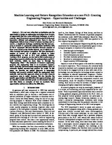

![[PDF] Download Pattern Recognition and Machine Learning ...](https://m.moam.info/img/260x300/pdf-download-pattern-recognition-and-machine-learn_64785ad5097c4796708cb7b3.jpg)


![[PDF] Pattern Recognition and Machine Learning - Google Sites](https://m.moam.info/img/260x300/pdf-pattern-recognition-and-machine-learning-googl_64770ec9097c474d228b8fc6.jpg)

![[PDF] Pattern Recognition and Machine Learning (Information Science ...](https://m.moam.info/img/260x300/pdf-pattern-recognition-and-machine-learning-infor_64786698097c4744708cc9f7.jpg)
![[PDF] Pattern Recognition and Machine Learning - Google Sites](https://m.moam.info/img/260x300/pdf-pattern-recognition-and-machine-learning-googl_6477bc3c097c4737708c07c0.jpg)


![[PDF] Pattern Recognition and Machine Learning (Information Science ...](https://m.moam.info/img/260x300/pdf-pattern-recognition-and-machine-learning-infor_6478594c097c474b228d1897.jpg)


