Pattern Recognition Via Vasconcelos’ Genetic Algorithm Angel Kuri-Morales Instituto Tecnológico Autónomo de México. Río Hondo No.1, Tizapán San Angel, C.P. 01000, MÉXICO.
[email protected]
Abstract. In this paper we describe a heuristic approach to the problem of identifying a pattern embedded within a figure from a predefined set of patterns via the utilization of a genetic algorithm (GA). By applying this GA we are able to recognize a set of simple figures independently of scale, translation and rotation. We discuss the fact that this GA is, purportedly, the best among a set of alternatives; a fact which was previously proven appealing to statistical techniques. We describe the general process, the special type of genetic algorithm utilized, report some results obtained from a test set and we discuss the aforementioned results and we comment on these. We also point out some possible extensions and future directions
1 Introduction In [1] we reported on the application of the so-called Eclectic Genetic Algorithms applied to the problem of pattern recognition. In this paper we offer new insights via the so-called Vasconcelos’ GA. The problem of pattern recognition has long been considered to be a topic of particular interest in many areas of Computer Science. It has been tackled in many ways throughout a considerably large span of time and, as of today, it remains a subject of continuous study. In this paper we report yet another method to solve a particular problem of pattern recognition. This problem may be described as follows: a) We are given a certain graphical figure, possibly composed of an unknown nonlinear combination of simpler (component) graphical figures. For our discussion we shall call this figure the master figure or, simply, the master. b) We are given a set of "candidate" figures, which we are interested to discover within the master if any of these does indeed "lie" within it. What we mean when we say that a figure lies within another figure is, in fact, central to our method and we shall dwell upon this matter in what follows. We shall call these possibly embedded figures the patterns. c) We would like to ascertain, with a given degree of certainty, whether one or several of the patterns lie within the master.
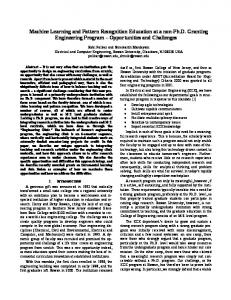
1.1 General Process In figure 1, a set of patterns is shown surrounding a master. The main problem of defining when a pattern lies within a master is interesting only when such relation is not direct. That is, it is relatively simple to find, say, a square within a master if such a square is one of the patterns on a 1 to 1 scale, in the same position and with the same inclination. Here, however, we are looking for a much more general case. Namely, we impose upon our method, the task of identifying a pattern in the master even if the pattern is found on a different scale, a different position and a different inclination than the ones in the pattern. We shall define, therefore, three operators on the pattern: 1. A scale operator, which we denote by σ(s, f) , where s is the scale factor and f is the figure being scaled.
Fig. 1. A Set of Patterns and a Master.
2. A rotation operator, which we denote by ρ(r, f) , where r is the rotation angle, and f is the figure being rotated. 3. A translation operator which we denote by τ( t1 , t 2 , f) , where t1, t2 are the translations on the x and y axis respectively and f is the figure being translated. Henceforth, a pattern is mapped an arbitrarily selected number of times under scaling, rotation and translation into a derived pattern or descendant. That is, from every pattern we extract a family of descendants which arise from a process of repeated application of σ, ρ and τ . The i-th descendant ( δi (f) ) is denoted by
δi (f) = σi {si , ρi [ r i , τi ( t i1 , t i2 , f)]}
(1)
where the operators are successively applied to a figure f. The rationale behind this strategy is simple: under the assumption that the possible number of configurations is sufficiently large, we settle with a sample of the configuration space in the hope of capturing the essence of the pattern in all its possible states where by "state" we mean any one of the possible combinations of s, r, t1, t2. Clearly the number of possible states is sufficiently large so that an exhaustive enumeration of these is impractical. The size of the sample is largely determined, therefore, by practical considerations such as the amount of information contained in
the figure, the speed of the computer where the process of identification is performed and the amount of memory at our disposal. We denote the family of descendants for a given figure f by φ (f) . Once the samples (one per pattern) are obtained, we attempt to characterize the relationship between the i-th pattern and the master by minimizing a norm which should reflect the distance between the master and the pattern. If the said distance is minimum we shall accept the fact that the pattern is embedded within the master. This is what we mean when we say that a pattern lies within a figure. We shall accept that pattern f is found in the master m if the distance between f and m is relatively small. We could have, of course, attempted to minimize such distance from a "traditional" norm such as L1, L2 of L ∞ . Indeed, such a scheme was applied in [2] where we attempted to minimize the said distance in L ∞ . There we recognized a set of fuzzy alphabetic (i.e. A, B, ..., Z, ...) characters with a neural network and with a scheme similar to the one reported here. There, however, the patterns were unique. That is, the master consisted of only one of the fuzzified characters and the method performed unsatisfactorily when several patterns were put together. Our conclusion was that the problem lied in the fact that φ (f) was not sufficiently rich and/or the master was too complex. In order to overcome the limitations outlined above we felt it necessary to enrich φ and to adopt an ad hoc distance norm. To achieve these two goals while retaining the essence of the method we appealed to a genetic algorithm. In the algorithm a set of random patterns (each of which will act as a probe π ) is generated. Thus, information is maximized to begin with. That is, in terms of a Fourier decomposition no harmonics of the pattern are left out. Then the distance between the test pattern and both φ and the master is minimized simultaneously. To do this: a) The average distance from ∆δ =
∆δ between the probe ( π ) and each of the δ i is calculated
1
∑ (π - δi ) . N i b) The distance ∆ m between
π
and the master is calculated from ∆ m = π - m . 1 c) A mutual distance ∆ δm is derived from ∆ δm = ( ∆ δ + ∆ m ) . 2 The genetic algorithm receives as its initial population, therefore, a set of random patterns. Its fitness function is then the mutual distance ∆δm , which it tries to minimize. The population, thereafter, evolves to a fittest individual, which is constantly closer to both the set of descendants and the master, thereby establishing an informational meaningful link between the particular sample from which φ (f) originally arose and the master. In order to calculate the above mentioned distances the system is fed a set of figures in compressed (PCX) format. This set comprises both the master and the patterns. As a second step, the δ i are generated. Once having these samples (the arguments of the operators are generated randomly) the genetic string of the master and the descendants is composed of the a concatenation of the rows of the pattern (1 bit per pixel). The distance
between probe and descendants, on the one hand, and probe and master, on the other, is trivially calculated by counting those positions where the values agree. In our test we only considered black and white images. Therefore, an empty space is a "1", whereas a filled space is a "0". It should be clear that the genetic algorithm is basically measuring the information content coincidence in the probe vs. the descendants and vs. the master. It should also be clear that the fact that pattern information is state independent given a properly selected size of the sample. That is, regardless of where the pattern may be within the space of the master and regardless of its position and/or angle of inclination relative to the master, as long as the information of the pattern remains a match will be found, that is, as long as the pattern is not deformed.
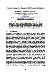
2 Genetic Algorithm For those familiar with the methodology of genetic algorithms it should come as no surprise that a number of questions relative to the best operation of the algorithm immediately arose. The Simple Genetic Algorithm frequently mentioned in the literature leaves open the optimal values of, at least, the following parameters: a) Probability of crossover (Pc). b) Probability of mutation (Pm). c) Population size. Additionally, premature and/or slow convergence are also of prime importance [3]. In the past we have conducted experiments [4] which led us to take the following decisions: a) We utilize Vasconcelos’ scheme, i.e. selection is deterministic on an extreme crossover schedule with N-elitism. b) Crossover is annular. c) Mutation is uniform. In what follows we describe in more detail the points just outlined. 2.1 The “Best” Genetic Algorithm Optimality in GA's depends on the model chosen. For reasons beyond the scope of this paper (but see reference [5]) we have chosen to incorporate in our model the following features: 2.1.1 Initial population It was randomly generated. We decided not to bias the initial population in any sense for the reasons outlined above. For these work we selected initial populations of size 50. 2.1.2 Elitism All of the individuals stemming from the genetic process are rated according to their performance. It has been repeatedly shown that elitism leads to faster convergence. Furthermore, simple elitism (and stronger versions) guarantee that the algorithm converges to a global optimum (although time is not bounded, in general). In figure 2 we
show the kind of elitism implemented. This is called “full” elitism, where the best N individuals of all populations (up to iteration t) are kept as those of the initial population of iteration t+1. 2.1.3 Selection The individuals are selected deterministically. The best (overall) N individuals are considered. The best and worst individuals (1-N) are selected; then the second best and next-to-the-worst individuals (2-[N-1]) are selected, etc.
Fig. 2. Full Elitism
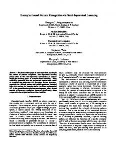
This is known as Vasconcelos’ model of GA's. Vasconcelos’ model has shown to guarantee that there is no premature convergence and that, as a consequence, it reaches generally better results than other models. Vasconcelos’ coupling scheme is illustrated in figure 3. 2.1.4 Crossover. It is performed with a probability Pc. In our GA Pc = 0.9 . Further, we adopted annular crossover. Annular crossover makes this operation position independent. In the past several authors [6] have attempted to achieve position independence in the genome. Annular crossover allows for unbiased building block search, a central feature to GA's strength. Two randomly selected individuals are represented as two rings (the parent individuals). Semi-rings of equal size are selected and interchanged to yield a set of offspring. Each parent contributes the same amount of information to their descendants. 2.1.5 Mutation Mutation is performed with probability Pm =0.005. Mutation is uniform and, thus, is kept at very low levels. For efficiency purposes, we do not work with mutation probabilities for every independent bit. Rather, we work with the expected number of mutations¸ which, statistically is equivalent to calculating mutation probabilities for every bit. Hence, the expected number of mutations E(m) is calculated from E(m) = Pm × l × N ,
where l is the length of the genome in bits and N is the number of individuals in the population. Since the pattern representation consisted, in our case, of a 5625 bit long binary string( l = 5625), Pm=0.005 and N=50 we have that E(m) = 1,406, i.e. in every generation 1,406 (out of 281,250) bits are randomly selected and complemented ( 0 → 1 and 1 → 0 ).
Fig. 3. Deterministic Coupling
3 Experiments We performed an initial set of experiments to test the scheme we have described. We designed 5 sets of 10 descendants each: Φ1 (f 1), Φ1 (f 2), Φ1 (f 3), Φ1 (f 4), Φ1 (f 5) and 5 sets of 25 descendants each: Φ2 (f 1), Φ2 (f 2), Φ2 (f 3), Φ2 (f 4), Φ2 (f 5) . The descendants were obtained by applying operators σ and τ as described above. These we matched vs. a master figure (the patterns and the master figure correspond to the ones shown in Figure 1.). The two following tables show the results for these experiments. The selection criterion is actually very simple: accept as an embedded pattern the one which shows the smallest ∆δm . In tables 1 and 2, the smallest ∆ δm correspond to patterns 1 and 3, which are shown in Figure 1. The patterns not recognized are shown in the same figure. The master figure is shown in Figure 4. As seen, in this simple trial the correlation between the matches and what our intuition would dictate is accurate. This results are encouraging on two accounts: First, it would seem that the method, in general, should be expected to yield reasonably good results. Second, from the tables, it seems that whenever φ (f) is enriched, the precision is enhanced.
Table 1. Results for Φ 1 .
Table 2. Results for Φ 2 .
Table 3. Master Figure
4 Conclusions In the method described above the genetic algorithm, by its own definition evolves under supervision of the environment [7], via the fitness function. However, the fitness function itself has been determined by a random sampling of the possible space of solutions. In that sense the search is unsupervised, in as much as the way the spectrum of the restricted sample space is "blind". Although we have proven that Vasconcelos’
model is superior to alternative ones [8] still much work remains to be done. In the first place, the patterns and the master were specifically selected to validate the model in first instance. The figures that we attempted to recognize were directly embedded in the master. What would happen if the sought for relationship were not so straightforward? We intend to pursue further investigation along these lines. Secondly, although the results of the model, as reported, correspond to intuition, it is not clear that this intuition could be substantiated in general. For example, are we sure that the figure in pattern 4, for instance, is not informationally contained in the master? Thirdly, the measure that we used is amenable to reconsideration and enrichment. Do we have certainty that this direct difference is the best norm? We remarked earlier that a way to ensure that this norm is adequate is that the algorithm itself selects it. This is true in the sense that the genetic methodology assigns a certain degree of fuzziness to the measure. For example, the random walk implicit in the GA translates into the fact that the distance being minimized is adaptive. Similar distances (but not identical) would have been obtained by slight changes in the initial conditions set in the GA. Finally, the technical details were quite interesting in themselves. The mere process of applying the defined operators ρ, σ and τ became an interesting matter. The figures were to remain within the boundaries of the master's environment; the discreetness of the binary mapping disallowed certain arguments s, r and t1, t2; the repeated comparison of the probe vs. the patterns in implied vast amounts of computation. In view of the technical shortcomings of the method, it remains to generalize it and prove its universality before attempting to solve large practical problems with it. We hope to report on the (successful) completion of the investigation shortly.
References 1. 2. 3. 4.
5. 6. 7. 8.
Kuri, A., “Pattern Recognition via a Genetic Algorithm”, II Taller Iberoamericano de Reconocimiento de Patrones, La Habana, Cuba, pp. 127-133, Mayo, 1997. Fernández-Ayala, A., Implementación de una Red Neuronal Multi-Capa para el Reconocimiento de Patrones, Tesis de Maestría, Instituto de Investigaciones Matemáticas Aplicadas y Sistemas, 1991. Mühlenbein, Gorges-Schleuter & Krämer: Evolution Algorithms in combinatorial optimization, Parallel Computing, Vol. 7, pp. 65-85, 1988. Kuri, A., “Penalty Function Methods for Constrained Optimization with Genetic Algorithms: a Statistical Analysis”, Lectures Notes in Artificial Intelligence No. 2313, pp. 108-117, Coello, C., Albornoz, A., Sucar, L., Cairó, O., (eds.), Springer Verlag, April 2002. Goldberg, D., Genetic Algorithms in Search, Optimization and Machine Learning, Addison-Wesley Publishing Company, 1989. Vose, M., Generalizing the notion of schema in genetic algorithms, Artificial Intelligence, 50, (1991), 385-396. Tsypkin, Ya. Z., Neural Networks and Fuzzy Systems, p. 179, Prentice-Hall, 1993. Kuri, A., “A Methodology for the Statistical Characterization of Genetic Algorithms”, Lectures Notes in Artificial Intelligence No 2313, pp. 79-89, Coello, C., Albornoz, A., Sucar, L., Cairó, O., (eds.), Springer Verlag, April 2000.