Patterns and dynamics in transitional plane Couette flow - University of ...

PHYSICS OF FLUIDS 23, 041301 共2011兲

Patterns and dynamics in transitional plane Couette flow Laurette S. Tuckerman1,a兲 and Dwight Barkley2,1,b兲 1

PMMH (UMR 7636 CNRS-ESPCI-UPMC Paris 6-UPD Paris 7), 10 rue Vauquelin, 75005 Paris, France Mathematics Institute, University of Warwick, Coventry CV4 7AL, United Kingdom

2

共Received 4 January 2011; accepted 22 March 2011; published online 19 April 2011兲 Near transition, plane Couette flow takes the form of large-scale, oblique, and statistically steady alternating bands of turbulent and laminar flow. Properties of these flows are investigated using direct numerical simulation in a tilted computational domain. Four regimes—uniform, intermittent, periodic, and localized—are characterized. The Fourier spectrum along the direction of variation of the pattern is presented, and the component corresponding to the pattern wavenumber is investigated as an order parameter. The mean flow of a periodic pattern is characterized and shown to lead to a relation between the Reynolds number and the wavelength and angle of a pattern. © 2011 American Institute of Physics. 关doi:10.1063/1.3580263兴 I. INTRODUCTION

Transition to turbulence in wall-bounded shear flows has attracted the attention of a large number of researchers using a range of approaches. The three classic wall-bounded shear flows are plane Couette, plane Poiseuille, and pipe flow. This list can be broadened to include counter-rotating Taylor– Couette flow, boundary layer flow, and the flow between differentially rotating disks. The classic tool of linear stability analysis is not useful under these circumstances since the transition to turbulence takes place far from any linear instability. Transitional flows contain turbulent regions, called spots, slugs, puffs, and bands, which coexist with laminar regions. This leads to questions concerning sizes or wavelengths and growth or decay. A particular coexistence regime consists of alternating turbulent and laminar bands. Both the wavelength and the angle between the bands and the streamwise direction are well-defined and depend on the Reynolds number. The discovery of regular turbulent-laminar patterns dates from about 2000 by Prigent and Dauchot1–4 in counterrotating Taylor–Couette flow, although more irregular versions were observed as early as the 1960s by Coles5 and Van Atta6 and later by Andereck et al.,7 Hegseth et al.,8 and Goharzadeh and Mutabazi.9 Turbulent-laminar banded patterns were subsequently observed in experiments on plane Couette flow1–4 and rotor-stator flow,10 and in numerical simulations of plane Couette flow,11–19 of plane Poiseuille flow,20,21 and of counter-rotating Taylor–Couette flow.22–24 We have studied various aspects of turbulent-laminar banded patterns in plane Couette flow by simulating the Navier–Stokes equations in a rectangular computational box, aligned with the direction of the pattern wavevector. This article summarizes what we have learned about these remarkable flows. II. GEOMETRY AND COMPUTATIONS

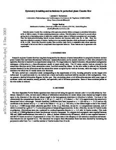
Figure 1 shows a visualization of one of our computed a兲

Electronic mail: [email protected]. Electronic mail: [email protected].

b兲

1070-6631/2011/23共4兲/041301/9/$30.00

turbulent-laminar banded patterns at a Reynolds number of 350, more specifically the kinetic energy halfway between the two bounding plates. The small-scale structure seen in Fig. 1 within the turbulent bands is a manifestation of the streamwise vortices and streaks that comprise turbulence in wall-bounded shear flow.25–27 Figure 2, a spatiotemporal diagram of the variation of the streamwise velocity along the spanwise direction, shows both the dynamic nature of smallscale spatial and temporal features as well as the long-lived nature of the large-scale banded structure. In Fig. 1, the distance between successive turbulent bands is ␭ = 40, and the angle between the bands and the streamwise direction is ␪ = 24°, approximately as found in experiment. This angle is actually imposed by our calculation, as we now describe. The distance between bands is very large compared to the small-scale variation within the bands, and so we choose our domain to be long in the direction of the pattern

FIG. 1. 共Color online兲 Computed turbulent-laminar pattern at Re= 350. Shown is the kinetic energy at y = 0, midway between bounding plates at y = ⫾ 1 which move to the right and left in the streamwise direction. Turbulent bands consist of streamwise streaks and vortices. The bands are oriented in the direction denoted by x at an angle of 24° from the streamwise direction, and are separated by a wavelength of 40 in the direction of the pattern wavevector, denoted by z.

23, 041301-1

© 2011 American Institute of Physics

Downloaded 26 Apr 2011 to 193.54.81.244. Redistribution subject to AIP license or copyright; see http://pof.aip.org/about/rights_and_permissions

041301-2

Phys. Fluids 23, 041301 共2011兲

L. S. Tuckerman and D. Barkley

300

t 0

0

spanwise

120

FIG. 2. Streamwise velocity along a line oriented in the spanwise direction in the midplane at Re= 350. Streaks move out from the center of the turbulent region toward the laminar regions. The flow is the same as that in Fig. 1.

wavevector and short in the direction parallel to the bands. That is, our computational domain is rectangular, but tilted with respect to the streamwise and spanwise directions. Figure 1 has been constructed by filling a square oriented along the streamwise-spanwise axes with multiple copies of our tilted rectangular computational domain. Although our computational domain effectively imposes the angle, the wavelength may be any divisor of the domain length in the direction of the pattern wavevector. We call the directions parallel to the bands and to the expected pattern wavevector x and z, respectively, with lengths Lx and Lz. Our other definitions are conventional: y is the cross-channel direction, with Ly taken to be 2. Thus, laminar Couette flow between plates translating in opposite directions and located at y = ⫾ 1 is UCou = y共cos ␪ex + sin ␪ez兲,

共1兲

which, just as in the conventional orientation, is trivially a zero-pressure-gradient solution to the Navier–Stokes equations since 共UCou · ⵜ兲UCou = 0 = ⵜ2UCou .

FIG. 3. 共Color online兲 Timeseries in domain with Lz = 120. Middle: spanwise velocity at 32 points along a line in the midplane x = y = 0 as the Reynolds number is decreased. Left: modulus of Fourier transform in the z direction, averaged over time windows of length ⌬T = 1000, showing evolution of components corresponding to wavelengths of 40 共solid red兲, 60 共long-dashed blue兲, 120 共short-dashed green兲, and ⬁ 共dotted black兲. Right: evolution of spanwise velocity within laminar 共left兲 and turbulent 共right兲 bands over interval of length ⌬T = 1000. Transition to an intermittent regime is seen at Re= 410, to three bands at Re= 390, to two bands at Re= 310, to a localized state at Re= 300, and to laminar Couette flow at Re= 290.

共2兲

We either take Lz to be ␭ = 40, the pattern wavelength, or to be 3␭ = 120. The length Lx is chosen to satisfy a geometric constraint based on the streamwise vortices and streaks that maintain turbulence.25–27 Near threshold, these vortices and streaks have a spanwise wavelength of 2Ly ⬇ 4. To accommodate an integer number of these requires Lx sin ␪ ⬇ 4. To solve the Navier–Stokes equations, our computations use Prism,28 in which the 共x , y兲 plane is discretized by spectral elements and the z direction by Fourier modes. The code is parallelized across the Fourier direction. Periodic boundary conditions are imposed in the x and z directions, and no-slip boundary conditions in the y direction. Typical computations use Nx ⫻ Ny ⫻ Nz = 81⫻ 41⫻ 512= 1.7⫻ 106 points or modes to resolve a domain of size Lx ⫻ Ly ⫻ Lz = 10⫻ 2 ⫻ 40 and Nx ⫻ Ny ⫻ Nz = 61⫻ 31⫻ 1024= 1.9⫻ 106 points or modes for domains with Lx ⫻ Ly ⫻ Lz = 10⫻ 2 ⫻ 120. III. FOUR REGIMES

Our numerical computations, like the physical experiments, are conducted by lowering the Reynolds number. Figures 3 and 4 are spatiotemporal diagrams, taken along the line x = y = 0, where the velocity is zero for laminar plane Couette flow 共1兲. We show timeseries of the spanwise velocity at 32 equally spaced points in the z direction for a simulation in a domain of size Lz = 120, Lx = 10 as the Reynolds

FIG. 4. 共Color online兲 As in Fig. 3, but with slightly different Reynolds number history. Two turbulent bands disappear at Re= 320, leading to translation of the single remaining band with the eventual reappearance of a stationary pattern with two bands.


041301-3


Patterns and dynamics in transitional plane Couette flow

number is lowered in discrete steps. The accompanying graph along the left shows the moderate-time 共⌬T = 1000兲 average of the first Fourier components m = 0 , 1 , 2 , 3 共i.e., wavelengths ⬁, 120, 60, and 40兲 in the z-direction. The insets on the right show expanded versions of portions of the timeseries for z locations in the laminar and the turbulent regions. The terms “turbulent” and “laminar” can be taken here to mean strongly and weakly chaotic, respectively. That is, the turbulent region does not display a Kolmogorov spectrum and the laminar region is not described by the linear plane Couette profile, as shown by the expanded timeseries in Fig. 3. Figure 2 illustrates the detailed behavior of the flow within the two regions. We define four turbulent patterned regimes, which we call uniform, intermittent, periodic, and localized, listed in order of decreasing Reynolds number. 共i兲 In the uniform regime, turbulence extends across the entire domain, whereas 共ii兲 in the intermittent regime, laminar patches appear and disappear. 共iii兲 In the periodic regime, laminar and turbulent regions are permanent. Although there is small-scale stochastic motion, large-scale motion of the bands is slow or absent. The spatial periodicity is well-defined. 共iv兲 In the localized regime, a single turbulent region is surrounded by laminar flow. In this case, the turbulent region is exponentially localized in space and the laminar region is in fact described by the linear plane Couette profile. We point out some particular events that can be seen in Fig. 3. At Re= 310, the number of turbulent bands is reduced from three to two; simultaneously the Fourier component corresponding to wavelength 40 is succeeded by that of wavelength 60. At Re= 300, the number of bands is further reduced to one. However, this is not a manifestation of a periodic pattern with wavelength 120, but a localized state, in which the turbulent region can be surrounded by a laminar region of any width. This is demonstrated11 by producing a pattern containing a single turbulent band of the same width in domains varying from Lz = 30 to Lz = 120. Correspondingly, no single Fourier component dominates in this regime. In Fig. 4, two turbulent bands disappear at Re= 320, whereupon the single remaining band moves leftward, periodically emitting the root of a turbulent band. Eventually, one of these succeeds and a stationary pattern with two bands is established. At Re= 300, the number of bands is further reduced to one, and finally below Re= 290 only the laminar state remains. The formation process of turbulent-laminar banded patterns in a large-aspect-ratio domain with streamwise and spanwise extents of Lstr = 800 and Lspan = 356, in which the orientation of the turbulent bands arises out of initial conditions, is well documented by Duguet et al.16 Competition between patterns with different wavelengths or orientations is characterized by Prigent et al.1–4 and by Rolland and Manneville.18 IV. TRANSITION BETWEEN UNIFORM, INTERMITTENT, AND PERIODIC PATTERNS

As shown in Figs. 3 and 4, the Fourier transform in the z direction provides a good quantitative measure for distin-

guishing between the different turbulent-laminar patterns. In this section we present simulations carried out in a domain of length Lz = 40, just large enough to accommodate a single wavelength, for fixed Reynolds numbers. Figure 5 shows timeseries and spectra for simulations carried out over 20 000 time units at Reynolds numbers of 350, 410, and 500. The first row presents spatiotemporal diagrams like those in Figs. 3 and 4 of the spanwise velocity along a line in the z direction in the midplane. The next row presents Fourier transforms in the z direction of this spanwise velocity. These differ from those included in Figs. 3 and 4 as follows. First, we show the square modulus of the entire spectrum, rather than the first few components. Second, we average the instantaneous Fourier components over the entire simulation, rather than over intervals on the order of 100. The peak at m = 1, i.e., at a wavelength of 40, corresponds to the turbulent-laminar pattern, most prominent at Re= 350, reduced at 410 and barely present at 500. This component is plotted as a function of Re in Fig. 6. The last row of Fig. 5 shows the spectrum of the streamwise velocity. The m = 1 component is still very prominent at Re= 350 and 410, but there are additional peaks at 7 ⱗ m ⱗ 11 for all three Reynolds numbers. These components reflect the small-scale structure seen in Figs. 1 and 2. At these Reynolds numbers, a streamwise vortex occupies approximately the entire gap 共Ly = 2兲 with an equal spanwise extent, leading to a pair of vortices whose spanwise width is 4, with an extension in the z direction of 2 ⫻ Ly / cos共␪兲 = 4 / cos共24°兲 = 4.38, or a Fourier component of 40/ 4.38= 9.1. The streamwise vortices in turn lead to streaks, meaning that they advect high and low streamwise velocity toward the midplane from near the bounding plates. The absence of peaks corresponding to small-scale structure in the spanwise spectrum confirms this heuristic picture: while a streamwise vortex should have substantial spanwise velocity, the corresponding velocity in the midplane should be primarily in the y direction. We return to the m = 1 Fourier component of the spanwise velocity and now consider the probability distribution of its instantaneous values. The Fourier component has both an amplitude a and a phase ␾, but, by translational symmetry, its probability distribution ␳ must be independent of phase, i.e., of the location along the z axis. We write

共3兲 We estimate p共ai兲 via p共ai兲 ⬇

1 ai⌬a

冕

ai+⌬a/2

ai−⌬a/2

ada

冕

2␲

d␾␳共a, ␾兲,

共4兲

0

where the integral in Eq. 共4兲 is estimated by counting the proportion of values of a falling within each of 20 bins of width ⌬a centered on ai. Figure 7 shows p共a兲 obtained from timeseries for Re = 350, 410, and 500 on a logarithmic scale, along with fits of


041301-4



FIG. 5. 共Color online兲 Left column: statistically steady turbulent-laminar pattern at Re= 350. Middle column: intermittent state at Re= 410. Right column: uniform turbulence at Re= 500. Top row: timeseries of the spanwise velocity along the line x = y = 0 at 32 equally spaced values of z. Middle row: time-average of the power spectrum in z of the spanwise velocity. Bottom row: time-average of the power spectrum of the streamwise velocity. The blue square at m = 1 corresponds to the pattern wavelength of 40. The red triangles at 7 ⱗ m ⱗ 11 correspond to streamwise streaks. The m = 0 component is shown as a black cross and the remaining components are shown as green dots.

ln p共a兲 to even polynomials. At Re= 500, when the turbulence is uniform, p共a兲 has a clear maximum at a = 0; it is in fact extremely well fit by a Gaussian ln p共a兲 = c0 + c2a2 .

共5兲

The probability distribution function is almost identical for 500ⱕ Reⱕ 600.29 The most probable value shifts from 0 to

positive a as Re is lowered, attaining values near 1 共on an arbitrary scale兲 for Re= 350. We generalize Eq. 共5兲 to a quartic polynomial ln p共a兲 = c0 + c2a2 + c4a4 .

共6兲

In the usual scenario for phase transitions, c4 would vary little with Re while c2 would change sign at the transition.


041301-5



FIG. 6. 共Color online兲 Square modulus of Fourier component corresponding to pattern wavelength as a function of Reynolds number.

However, a quartic polynomial does not provide a good fit for the patterned flows, as exemplified by the curve for Re = 350. Weighting the points by their probability changes the fit, but does not improve it. Figure 8 shows the coefficients of the fit 共6兲 as a function of Re. The coefficients change very little for Reⱖ 500 and within the range 350ⱕ Re ⱕ 370. The coefficients change dramatically within 410 ⱕ Reⱕ 430: c4 decreases to near zero and c0 and c2 exchange signs. The most probable value amax is difficult to determine at intermediate values because p共a兲 is flat and contains noise. Therefore, we take amax to be the maximum value of the quartic function 共6兲, or 0 if 兩c4兩 ⬍ 0.1, i.e.,

FIG. 7. 共Color online兲 Logarithm ln p共a兲 for the modulus a of the first Fourier component, for a uniformly turbulent flow at Re= 500, an intermittent flow at Re= 410, and a turbulent-laminar patterned flow at Re= 350. The most probable value is a = 0 for uniform turbulence but has a finite value for a patterned flow. Points are obtained by Fourier transforming and binning the data in Fig. 5. Curves are fits to quartic functions.

FIG. 8. 共Color online兲 Top: fitting coefficients for quartic functional form 共6兲. Quartic coefficient c4 becomes negligible for Reⱖ 430, coefficients c0, c2 change sign near this value as well. Bottom: most probable value of a is zero for Reⱖ 430.

amax =

再

0

if 兩c4兩 ⬍ 0.1

− c2/2c4

otherwise.

冎

共7兲

Any of these—the amplitude of amax or c4 or the sign of c0, c2—can be used as an order parameter for the existence of a turbulent-laminar banded pattern. V. OTHER DOMAINS

Although we have primarily studied the case ␪ = 24°, we have also studied other angles. A summary of our survey in Re and ␪ is given in Fig. 9. Figure 10 shows stationary patterned states, some periodic and some localized, with extremal angles and wavelengths at Re= 350. By fixing ␪ = 24°

FIG. 9. 共Color online兲 Survey of turbulent-laminar patterned regimes in our computations of plane Couette flow as a function of imposed angle ␪ and Reynolds number Re. Uniform turbulence 共solid squares, red兲, intermittent 共green, crosses in squares兲, turbulent-laminar patterns with wavelength of 40 共blue, crosses兲 or 60 共light blue, dots兲, localized states 共stars, purple兲, laminar Couette flow 共hollow squares, yellow兲. Numbers show wavelengths found in experiments 共Ref. 3兲 at appropriate values of ␪ and Re.


041301-6



-

FIG. 12. 共Color online兲 Evolution in a domain with streamwise extent of 120 and spanwise extent of 4. Timeseries taken at points along long streamwise direction indicated by red line. Turbulence disappears throughout the domain for Reⱕ 385.

FIG. 10. 共Color online兲 Extremal turbulent-laminar banded patterns at Re = 350. Top row: ␪ = 24° with ␭ = 35 共left兲 and ␭ = 65 共right兲. Bottom row: ␪ = 15° and ␪ = 66°.

and Lx, and varying Lz, we produced turbulent-banded patterns with wavelengths between 35 and 65. By fixing Lz = 120 and varying ␪ and Lx according to Lx = 4 / sin ␪, we were able to produce patterns at angles between 15° and 66°. 共The pattern at 66° is a localized state.兲 We expect most of these states to be unstable in a less restricted domain. Figures 11 and 12 show simulations at the extremal angles of 0° and 90°, i.e., in more classic rectangular do-

mains aligned with the streamwise and spanwise directions. At ␪ = 0°, the spanwise extent is Lz = 120 and we have fixed the streamwise extent to Lx = 10. We see that turbulent patches subsist down to Re= 220, far lower than in the ␪ = 24° case. This is not a well-defined threshold; when simulations are continued at fixed intermediate Reynolds numbers from the intermediate fields in Fig. 11, turbulence persists in some cases and not in others. The Reynolds-numberbehavior of the threshold for turbulence is statistical and strongly dependent on the initial condition and the procedure.30,31 It is also extremely dependent on the dimensions of the domain. In computations of plane Couette flow in a domain similar to that in Fig. 11, Duguet17 also finds growth of turbulent patches at Reynolds numbers below 300, and suggests that this behavior is a manifestation of the unstable states located on homoclinic snaking branches computed by Schneider et al.32 In contrast, for ␪ = 90°, i.e., in a domain with a long streamwise extent of 120 and short spanwise length of 4, the flow becomes laminar throughout when Reⱗ 385 without passing through any intermediate pattern.

VI. MEAN FLOW OF A PERIODIC TURBULENTLAMINAR PATTERN

We now analyze in detail the mean flow corresponding to a well-established turbulent-laminar pattern at parameter values Re= 350, ␪ = 24°, and Lz = 40 using the data from the timeseries shown in Fig. 5 between t = 6000 and t = 8000. In this section, we calculate the time-average of the velocity field over the entire domain, rather than just the spanwise velocity at sampled points across a line at the midplane. This time-averaged velocity varies little in x, the direction parallel to the turbulent bands; it is therefore meaningful to average over x as well, defining 具u典共y,z兲 ⬅ FIG. 11. 共Color online兲 Evolution in a domain with streamwise extent Lx = 10 and spanwise extent Lz = 120. Timeseries taken at points along long spanwise direction indicated by red line. Turbulent regions subsist far below Re= 300.

1 TLx

冕冕 t0+T

Lx

dt

t=t0

dxu共x,y,z,t兲.

共8兲

x=0

The distinctive features of 具u典 = 共具u典 , 具v典 , 具w典兲 are best viewed by subtracting from it the basic Couette profile 共1兲 and by expressing the flow in the 共y , z兲 plane via a streamfunction, since ⳵y具v典 + ⳵z具w典 = 0,


041301-7



U (y, z) Ψ(y, z) Eturb (y, z) P (y, z)

FIG. 13. 共Color online兲 U共y , z兲: transverse component of mean flow. ⌿共y , z兲: streamfunction of in-plane mean flow. A long cell extends from one laminarturbulent boundary to the other. Gradients of ⌿ are much larger in y than in z, i.e., 兩W兩 Ⰷ 兩V兩. In the laminar region at the center, W , V ⬇ 0. Eturb共y , z兲: mean ˜ · ˜u典 / 2. There is a phase difference of ␭z / 4 = 10 between extrema of Eturb and U. P共y , z兲: mean pressure field. Pressure gradients are turbulent kinetic energy 具u primarily in the y direction and within the turbulent region. Color ranges for each field from blue to red: U 关⫺0.4, 0.4兴, ⌿ 关0, 0.09兴, Eturb 关0, 0.4兴, P 关0, 0.007兴.

具u典 = UCou + Uex + ⵜ ⫻ ␺ex .

共9兲

Figure 13 shows U and ␺ in the 共y , z兲 plane as well as the ˜ · ˜u / 2典 and the mean pressure 具p典. turbulent kinetic energy 具u The fields in Fig. 13 all display centro-symmetry, U共− y,− z兲 = U共y,z兲,

共10兲

where z = 0 is defined to be at the center of the turbulent region. As was demonstrated in Secs. III and IV, the z dependence is extremely well approximated by a single Fourier mode. This leads to representations of the form U共y,z兲 ⬇ U0共y兲 + Uc共y兲cos共2␲z/␭兲 + Us共y兲sin共2␲z/␭兲,

冉冊

1 2 ␲2 . ⵜ =O Re Re

共13兲

The nonlinear term is dominated by advection in the z direction by UCou. Evaluating it at a typical value y = 1 / 2, we obtain as an estimate for the nonlinear term 共具u典 · ⵜ兲 ⬇ ez · UCou⳵z ⬇ sin ␪ y

2␲ ␲ ⬇ sin ␪ . ␭ ␭

共14兲

A more complete justification13 of Eqs. 共13兲 and 共14兲 relies on the full computed fields and the functional form 共11兲. The balance between Eqs. 共13兲 and 共14兲 leads to

共11兲 involving only three scalar functions U0, Uc, and Us, where U0, Uc are odd in y and Us is even. A view of 具u典 in two streamwise-spanwise planes at y = ⫾ 0.725 is shown in Fig. 14. Computations of the mean flow and turbulent kinetic energy for turbulent-laminar banded patterns are presented by Tsukahara et al.21 for plane Poiseuille flow and by Dong22,23 for Taylor–Couette flow. The field 具u典 obeys the 共x , t兲-averaged Navier–Stokes equations whose x component is

共12兲 where ˜u ⬅ u − 具u典. Figure 15 shows the x components of these forces as a function of z at y = 0.725. In the laminar regions, the turbulent forcing term is absent. The nonlinear and viscous terms necessarily counterbalance one another; neither one is zero, as would be the case for UCou. Thus, it is clear that, even in the laminar region, 具u典 ⫽ UCou. The balance in the laminar region provides a basis for a quantitative relation between ␪, Re, and ␭. Because the wavenumber ␭ = 40 is long relative to Ly = 2, the Laplacian is dominated by variation in y, as in boundary layer theory, and the viscous term is very well approximated by

FIG. 14. Mean velocity components seen in three planes with standard orientation for Couette flow. The turbulent regions are shaded. Top: velocity components in the streamwise-spanwise plane at y = 0.725 共upper part of the channel兲. Middle: same except y = −0.725 共lower part of the channel兲. Bottom: flow in a constant spanwise cut. The mean velocity is shown in the enlarged region.


041301-8



VII. CONCLUSION

FIG. 15. 共Color online兲 Mean forces in x direction as a function of z at y = 0.725 for turbulent-laminar pattern at Re= 350. Advective −共U · ⵜ兲U ˜ · ⵜ兲u ˜ 典共black, 共blue, solid兲, viscous ⵜ2U / Re 共red, dashed兲, and turbulent −具共u short-dashed兲 forces. In the laminar region 共z ⬇ 0兲, the Reynolds-stress force vanishes and the viscous and advective forces are equal and opposite to one another.

Re sin ␪ = O共1兲. ␲␭

共15兲

Equation 共15兲 gives an order-of-magnitude relationship between Re, ␪, and ␭, as seen in Fig. 16, which includes experimental and numerical observations of plane Couette, Taylor–Couette, plane Poiseuille, and rotor-stator flow. A uniform definition of Reynolds numbers, angles, and wavelengths for these various flows is based on the average shear.3,13 For the numerical observations, the angles and wavelengths are highly constrained except in the case of Duguet et al.16

Turbulent-laminar patterns are a fascinating feature of many wall-bounded shear flows near transition. We have carried out detailed studies of turbulent-laminar patterns inplane Couette flow. Our main findings are as follows. First, turbulent-laminar banded patterns can be further divided into different regimes—intermittent, periodic, or localized. Second, the Fourier component corresponding to the pattern wavevector 共the direction we have called z兲 leads to the appropriate order parameter for describing such patterns. The transition from uniform turbulence to a turbulent-laminar pattern is described by a bifurcation in its probability distribution function. Third, the mean flow associated with a periodic turbulent-laminar pattern consists primarily of flow along the turbulent-laminar boundaries 共the direction we have called x兲, maintained by a weaker circulation around the turbulent regions. The mean balance of forces determines the relation between the angle, wavelength, and Reynolds number of the patterns. It seems plausible that studies of such patterns will lead to insights concerning the cause or nature of the fundamental problem of transition to turbulence. But even in the absence of such results, turbulent-laminar patterns are a perplexing and exotic object of study in their own right. ACKNOWLEDGMENTS

The authors thank O. Dauchot, Y. Duguet, P. Manneville, and A. Prigent for helpful discussions. This work was performed using high performance computing resources provided by the Grand Equipement National de Calcul IntensifInstitut du Développement et des Ressources en Informatique Scientifique project 1119. This paper is based on an invited lecture, which was presented by L.S.T. at the 62nd Annual Meeting of the Division of Fluid Dynamics of the American Physical Society, held 22–24 November 2009 in Minneapolis, MN. 1

FIG. 16. 共Color online兲 Re sin ␪ / 共␲␭兲 for turbulent-laminar patterns in experiment and computations in various wall-bounded shear flows. Experimental measurements by Prigent et al. 共Ref. 3兲 of plane Couette flow 共full black circles兲 and Taylor–Couette flow 共red crosses兲. Experimental measurements of rotor-stator flow by Cros and Le Gal 共Ref. 10兲共full blue triangles兲. Simulations of plane Poiseuille flow by Tsukahara et al. 共Refs. 20 and 21兲共full blue square兲. Simulations of Taylor–Couette flow by Meseguer et al. 共Ref. 24兲共hollow magenta pentagons兲 and by Dong 共Refs. 22 and 23兲共hollow magenta squares兲. Simulations of plane Couette flow by Duguet 共Ref. 16兲共hollow green circles兲, by Philips and Manneville 共Ref. 19兲共hollow magenta squares兲, and by Barkley and Tuckerman 共Ref. 13兲共black crosses兲.

A. Prigent, “La spirale turbulente: Motif de grande longueur d’onde dans les écoulements cisallés turbulents,” Ph.D. thesis, University Paris-Sud, 2001. 2 A. Prigent, G. Gregoire, H. Chaté, O. Dauchot, and W. van Saarloos, “Large-scale finite-wavelength modulation within turbulent shear flows,” Phys. Rev. Lett. 89, 014501 共2002兲. 3 A. Prigent, G. Gregoire, H. Chaté, and O. Dauchot, “Long-wavelength modulation of turbulent shear flows,” Physica D 174, 100 共2003兲. 4 A. Prigent and O. Dauchot, “Transition to versus from turbulence in subcritical Couette flows,” in IUTAM Symposium on Laminar-Turbulent Transition and Finite Amplitude Solutions, edited by T. Mullin and R. Kerswell 共Springer, Dordrecht, 2005兲, pp. 193–217. 5 D. Coles, “Transition in circular Couette flow,” J. Fluid Mech. 21, 385 共1965兲. 6 C. Van Atta, “Exploratory measurements in spiral turbulence,” J. Fluid Mech. 25, 495 共1966兲. 7 C. D. Andereck, S. S. Liu, and H. L. Swinney, “Flow regimes in a circular Couette system with independently rotating cylinders,” J. Fluid Mech. 164, 155 共1986兲. 8 J. J. Hegseth, C. D. Andereck, F. Hayot, and Y. Pomeau, “Spiral turbulence and phase dynamics,” Phys. Rev. Lett. 62, 257 共1989兲. 9 A. Goharzadeh and I. Mutabazi, “Experimental characterization of intermittency regimes in the Couette-Taylor system,” Eur. Phys. J. B 19, 157 共2001兲. 10 A. Cros and P. Le Gal, “Spatiotemporal intermittency in the torsional


041301-9


Couette flow between a rotating and a stationary disk,” Phys. Fluids 14, 3755 共2002兲. 11 D. Barkley and L. S. Tuckerman, “Computational study of turbulent laminar patterns in Couette flow,” Phys. Rev. Lett. 94, 014502 共2005兲. 12 D. Barkley and L. S. Tuckerman, “Turbulent-laminar patterns in plane Couette flow,” in IUTAM Symposium on Laminar-Turbulent Transition and Finite Amplitude Solutions, edited by T. Mullin and R. Kerswell 共Springer, Dordrecht, 2005兲, pp. 107–127. 13 D. Barkley and L. S. Tuckerman, “Mean flow of turbulent-laminar patterns in plane Couette flow,” J. Fluid Mech. 576, 109 共2007兲. 14 L. S. Tuckerman, D. Barkley, and O. Dauchot, “Statistical analysis of the transition to turbulent-laminar banded patterns in plane Couette flow,” J. Phys.: Conf. Ser. 137, 012029 共2008兲. 15 L. S. Tuckerman, D. Barkley, and O. Dauchot, “Instability of uniform turbulent plane Couette flow: Spectra, probability distribution functions and K − ⍀ closure model,” in Seventh IUTAM Symposium on LaminarTurbulent Transition, edited by P. Schlatter and D. Henningson 共Springer, New York, 2010兲, Vol. 18, pp. 59–66. 16 Y. Duguet, P. Schlatter, and D. S. Henningson, “Formation of turbulent patterns near the onset of transition in plane Couette flow,” J. Fluid Mech. 650, 119 共2010兲. 17 Y. Duguet, O. Le Maître, and P. Schlatter, “Stochastic and deterministic motion of a laminar-turbulent interface in a shear flow” 共private communication兲. 18 J. Rolland and P. Manneville, “Pattern fluctuations in transitional plane Couette flow,” J. Stat. Phys. 142, 577 共2011兲. 19 J. Philip and P. Manneville, “From temporal to spatiotemporal dynamics in transitional plane Couette flow,” Phys. Rev. E 83, 036308 共2011兲. 20 T. Tsukahara, Y. Seki, H. Kawamura, and D. Tochio, “DNS of turbulent channel flow at very low Reynolds numbers,” Proceedings of the Fourth International Symposium on Turbulence and Shear Flow Phenomena, 2005, pp. 935–940. 21 T. Tsukahara, K. Iwamoto, H. Kawamura, and T. Takeda, “DNS of heat

Phys. Fluids 23, 041301 共2011兲 transfer in a transitional channel flow accompanied by a turbulent puff-like structure,” in Proceedings of the Fifth International Symposium on Turbulence, Heat and Mass Transfer, Dubrovnik, Croatia, 25–29 September 2006, edited by Y. N. K. Hanjalić, Y. Nagano, and S. Jakirlić. 22 S. Dong, “Evidence for internal structures of spiral turbulence,” Phys. Rev. E 80, 067301 共2009兲. 23 S. Dong and X. Zheng, “Direct numerical simulation of spiral turbulence,” J. Fluid Mech. 668, 150 共2011兲. 24 A. Meseguer, F. Mellibovsky, M. Avila, and F. Marques, “Instability mechanisms and transition scenarios of spiral turbulence in Taylor-Couette flow,” Phys. Rev. E 80, 046315 共2009兲. 25 J. Jiménez and P. Moin, “The minimal flow unit in near-wall turbulence,” J. Fluid Mech. 225, 213 共1991兲. 26 J. M. Hamilton, J. Kim, and F. Waleffe, “Regeneration mechanisms of near-wall turbulence structures,” J. Fluid Mech. 287, 317 共1995兲. 27 F. Waleffe, “Homotopy of exact coherent structures in plane shear flows,” Phys. Fluids 15, 1517 共2003兲. 28 R. D. Henderson and G. E. Karniadakis, “Unstructured spectral element methods for simulation of turbulent flows,” J. Comput. Phys. 122, 191 共1995兲. 29 L. S. Tuckerman, D. Barkley, O. Moxey, and O. Dauchot, “Order parameter in laminar-turbulent patterns,” in Advances in Turbulence XII, Springer Proceedings in Physics Vol. 132, edited by B. Eckhardt 共Springer, New York, 2009兲, pp. 89–91. 30 S. Bottin, O. Dauchot, F. Daviaud, and P. Manneville, “Experimental evidence of streamwise vortices as finite amplitude solutions in transitional plane Couette flow,” Phys. Fluids 10, 2597 共1998兲. 31 A. Schmiegel and B. Eckhardt, “Persistent turbulence in annealed plane Couette flow,” Phys. Fluids 51, 395 共2000兲. 32 T. M. Schneider, J. F. Gibson, and J. Burke, “Snakes and ladders: Localized solutions of plane Couette flow,” Phys. Rev. Lett. 104, 104501 共2010兲.
