Psychological Review 2005, Vol. 112, No. 1, 60 –74
Copyright 2005 by the American Psychological Association 0033-295X/05/$12.00 DOI: 10.1037/0033-295X.112.1.60
Patterns of Continuity: A Dynamic Model for Conceptualizing the Stability of Individual Differences in Psychological Constructs Across the Life Course R. Chris Fraley
Brent W. Roberts
University of Illinois at Chicago
University of Illinois at Urbana–Champaign
In contemporary psychology there is debate over whether individual differences in psychological constructs are stable over extended periods of time. The authors argue that it is impossible to resolve such debates unless researchers focus on patterns of stability and the developmental mechanisms that may give rise to them. To facilitate this shift in emphasis, they describe a formal model that integrates 3 developmental processes: stochastic-contextual processes, person– environment transactions, and developmental constancies. The theoretical and mathematical analyses indicate that this model makes novel predictions about the way in which test–retest correlations are structured across a wide range of ages and test–retest intervals. The authors illustrate the utility of the model by comparing its predictions against meta-analytic data on Neuroticism. The discussion emphasizes the value of focusing on patterns of continuity, not only as phenomena to be explained but as data capable of clarifying the developmental processes underlying stability and change for a variety of psychological constructs.
Apted has not been alone in his search for an answer to this question. Psychologists have spent years mapping psychological development and tracing the unique pathways forged by people as they negotiate the vicissitudes of life (see Block, 1971; Bloom, 1964; Caspi & Roberts, 1999; Funder, Parke, Tomlinson-Keasey, & Widaman, 1993; Roberts & DelVecchio, 2000; Schuerger, Zarrella, & Hotz, 1989). Personality psychologists, for example, have focused on the stability of individual differences in personality traits, as commonly quantified by test–retest correlations (see Robins, Fraley, Roberts, & Trzesniewski, 2001). On the basis of this research we now know that certain aspects of childhood temperament correlate about .20 –.30 with adult personality characteristics (e.g., Block, 1993; Kagan & Moss, 1962). Moreover, research shows that personality traits appear to become increasingly stable over the life course, with children and young adults exhibiting less stability than older adults (Roberts & DelVecchio, 2000). In middle to late adulthood, for example, test–retest coefficients for basic personality traits often average around .50 –.80 (Costa & McCrae, 1994), whereas stability coefficients over equivalent periods of time in adolescence tend to be .30 –.50 (Roberts & DelVecchio, 2000). Although previous research has been able to establish some of the ways in which stability coefficients are patterned across the life course, both for personality traits and other psychological constructs, many psychologists continue to focus on the size of test– retest coefficients and, more specifically, on the question of whether the size of those coefficients suggests a small or large degree of stability. One of the arguments we make in this article is that the size of test–retest coefficients for a psychological construct has little to say about the kinds of processes that promote stability and change. Our objectives in this article are to demonstrate this point and to propose a theoretical model that highlights patterns of continuity and the developmental processes that give rise to them. We begin by discussing some of the limitations of point estimates of stability for addressing questions about developmental pro-
In 1963 Director Michael Apted and his colleagues interviewed 14 British 7-year-olds about their dreams, fears, and aspirations. The documentary that resulted, 7 Up, was a critically acclaimed film about the lives of a diverse group of children who would ultimately become Britain’s future (Almond & Apted, 1963). In the years that have followed, Apted has kept in touch with these individuals, interviewing them every 7 years about their relationships, accomplishments, and disappointments. The most recent update, 42 Up, was released in 1999. The 7 Up series is remarkable to watch because it allows the viewer to observe the unfolding of lives—from childhood to middle age— over the span of a few short hours. When watching this series, one cannot help but be struck by the degree of continuity that characterizes some of the children. The child interested in astronomy grows up to become a tenured professor of physics, and the timid, introspective child spends decades trying to discover his place in society. In contrast, other children exhibit marked discontinuities, coming across as arrogant and rebellious at age 21, for example, and humble and conventional 7 years later. The diversity of developmental trajectories captured by the series prompts the viewer to ask, “How stable are individual differences from infancy to adulthood?” Indeed, it is precisely this kind of question that Apted hoped to answer by working on the 7 Up series. Inspired by the Jesuit maxim “Give me the child until he is 7, and I will show you the man,” Apted sought to determine to what extent the personality of the child foreshadows that of the adult.
R. Chris Fraley, Department of Psychology, University of Illinois at Chicago; Brent W. Roberts, Department of Psychology, University of Illinois at Urbana–Champaign. Correspondence concerning this article should be addressed to R. Chris Fraley, who is now at the Department of Psychology, University of Illinois at Urbana–Champaign, Champaign, IL 61820. E-mail:
[email protected] 60
MODELING DEVELOPMENTAL MECHANISMS
cesses. As we show, point estimates often obscure information about the kinds of processes that may produce those estimates— information that is more readily revealed by focusing on patterns of coefficients across different ages and test–retest intervals. To facilitate this shift in emphasis, we discuss the patterns entailed by three processes that have been emphasized in the literature on psychological development: stochastic-contextual processes (e.g., Lewis, 1997, 1999, 2001a, 2001b), person– environment transactions (e.g., Caspi & Bem, 1990; Caspi, Bem, & Elder, 1989; Neyer & Asendorpf, 2001; Sameroff, 1975), and developmental constancies (e.g., Bowlby, 1973; McGue, Bacon, & Lykken, 1993; Roberts & Capsi, 2003; Roberts & Wood, in press). We show how these distinct processes can be conceptualized as elements of a more complete theoretical model and, via dynamic modeling and mathematical analysis (e.g., Haefner, 1996; Huckfeldt, Kohfeld, & Likens, 1982; van Geert, 1994), illustrate the novel kinds of patterns this theoretical model predicts. In doing so, we hope to demonstrate the value in focusing on patterns of continuity, not only as phenomena to be explained but as data capable of clarifying the developmental processes underlying stability and change for a variety of constructs of interest to psychological scientists.
Points and Patterns Researchers studying stability and change often assess variation in a psychological quality on two occasions and estimate the construct’s stability via a single test–retest coefficient. This approach carries with it two assumptions. The first is that the enduring nature of a psychological variable can be revealed by the
61
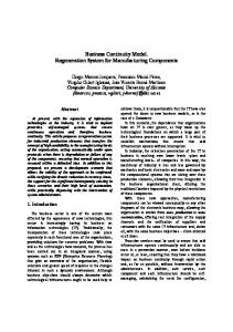
magnitude of its test–retest coefficient. This assumption is often explicit. In fact, much of the theory and research concerning individual differences is guided by the notion that stability coefficients should be high. The second assumption is that information about age or the duration of the test–retest interval is largely irrelevant to understanding psychological dynamics. This assumption is largely implicit but can be inferred by noting that most research tends to focus only on two assessment waves, and in cases in which more than one wave of data are available, researchers frequently aggregate all pairwise test–retest coefficients to yield a single, composite estimate of the stability of the construct under investigation. To see why both of these assumptions may be problematic, consider the histogram of test–retest coefficients diagrammed in the left-hand panel of Figure 1. These coefficients correspond to the stability of individual differences in the Big Five personality traits and are the same coefficients that Costa and McCrae (1994) analyzed when they concluded that personality traits do not change in adulthood. The average of these coefficients is approximately .65. This estimate, however, poses a number of interpretive ambiguities. For one, it is difficult to ascertain whether a value of .65 is consistent or inconsistent with the theoretical perspective under discussion because researchers rarely make point predictions (i.e., precise quantitative predictions) about the magnitude of the average test–retest coefficient that should be observed over time. A coefficient of .65 clearly indicates some degree of stability, but it is not clear whether this particular value is more consistent with a perspective that emphasizes instability (e.g., Lewis, 1999) over
Figure 1. Alternative explanations for stability and change. Left: A histogram of test–retest correlations that have been observed in adulthood for the Big Five personality traits. Right: Curves that fit these data but have dramatically different implications for the test–retest correlations over increasing test–retest intervals (in years). The solid curve illustrates a function that approaches zero in the limit; the dashed curve, in contrast, approaches a value of approximately .55.
62
FRALEY AND ROBERTS
stability (e.g., Costa & McCrae, 1994; McCrae et al., 2000). Although values of 0.00 or 1.00 have clear interpretations, values between these extremes comprise a vast gray area in which the implications of the data for theory become elusive. It is important to note, however, that there is additional information available to us that has the potential to inform our understanding of continuity and change. For example, if we disaggregate the coefficients in this example, it is possible to discern a pattern in which the magnitude of the coefficients decreases as the length of the test–retest interval increases (see the right-hand panel of Figure 1). This pattern is noteworthy because it suggests that the way in which personality traits change is systematic and, therefore, begs for a theoretical explanation. Moreover, with some imaginative extrapolation, one can envision alternative curves that not only capture these data but have different implications for data yet to be observed. For example, if these coefficients were to decrease to zero as the test–retest interval increases, as illustrated by the solid line in the right-hand panel of Figure 1, the implications for the study of personality development would be radically different than if the coefficients approached a nonzero asymptote, as illustrated by the dashed line. The former curve suggests that even if we can predict a person’s trait level with a high degree of accuracy over the span of a few months, we will not be able to do so over longer periods of time. Specifically, the predicted test–retest correlation approaches zero as the test–retest interval gets larger. The latter curve, in contrast, indicates that it might be possible to predict individual differences even over quite extended periods of time. Most important, this curve suggests that there is an enduring quality to the personality trait, although the overall magnitude of the stability coefficient is not very high. The observation that the stability coefficients may asymptote at different values suggests that the common assumption that the stability of a psychological variable is reflected in the size of any one test–retest correlation is incomplete and potentially misleading. Instead, we propose that the stability of a construct is reflected in the way in which its test–retest coefficients decay across increasingly long intervals or, more specifically, the way in which coefficients are patterned across a range of ages and test–retest intervals. It is possible for measurements to exhibit high test–retest correlations across two time points, but if these correlations approach zero as the test–retest interval increases, the psychological entity is clearly not an enduring one. It is important to note that this distinction can be captured only by attending to the pattern of test–retest coefficients; the magnitude of any one coefficient does not reveal the way in which the curves decay across time. As a consequence, a single coefficient has little to say about the dynamic processes that may underlie stability and change. We believe that psychological science would benefit enormously by treating such patterns as a valuable source of data—as not only phenomena that need explanation but also as phenomena that have the potential to provide insight into the kinds of developmental processes that give rise to continuity and change.
current knowledge about psychological continuity, researchers in the field must move beyond the current focus on the magnitude of test–retest correlations and begin taking into account the way in which those correlations are patterned across different ages and temporal intervals. In the following sections we take a first step in this direction by using empirical data on the stability of various personality traits to illustrate the kinds of patterns that exist in one area of psychological inquiry. Although we focus on the continuity of personality traits, it is important to emphasize that empirical patterns could be reconstructed for any kind of psychological construct for which people vary (e.g., anxiety, attachment security, attitudes, depression, intelligence, resilience, self-esteem, subjective well being, working memory capacity). We highlight basic personality traits here because of the extensive amount of longitudinal research that has accumulated in the study of personality trait development and our expertise in this specific area of research.1 For our illustration we reexamined the meta-analytic data originally compiled by Roberts and DelVecchio (2000). The details of their data set are reported in depth in their original article; therefore, we focus here on the novel ways in which we reconfigured and examined that data set. Roberts and DelVecchio were interested in whether personality trait stability tends to be higher in adulthood than in childhood. Accordingly, they meta-analyzed test–retest coefficients from a variety of longitudinal studies and regressed the magnitude of those coefficients on age, while holding constant the length of the test–retest interval. Although this strategy allowed Roberts and DelVecchio to address the way stability varies as a function of age, it does not allow one to consider the ways in which stability coefficients might be patterned over varying temporal intervals. To investigate such patterns, one must assemble a test–retest correlation matrix that captures the meta-analytic stability coefficients observed across numerous pairwise ages (e.g., age 1 to age 2, age 1 to age 10, age 23 to age 30). One advantage of reexamining this meta-analytic database in particular is that it contains information on a broad spectrum of personality traits—traits that have been organized according to the Big Five personality trait taxonomy (i.e., Extraversion, Agreeableness, Conscientiousness, Neuroticism, and Openness; John, 1990). Although some of the traits were not originally studied within the framework of the Big Five, it is useful to classify each trait as falling within one of the five categories to aid the synthesis and analysis of the patterns of continuity. In this sense, we are not examining the Big Five as objective entities but are using the taxonic qualities of the Big Five framework to facilitate the communication of findings across numerous personality trait measures. To construct a meta-analytic correlation matrix to characterize the stability of each personality trait across all available pairwise ages, we first rounded the ages for each assessment across studies to the nearest integer (e.g., age 3.7 became age 4). Next, for each of the five major trait domains (i.e., Extraversion, Agreeableness, Conscientiousness, Neuroticism, and Openness), we filled in as
Empirical Patterns of Continuity: An Illustration The observation that different theoretical functions can explain a single test–retest coefficient implies that it is impossible to understand the processes underlying psychological development without examining patterns of stability and change. To advance
1
We should note that even within the science of personality, trait approaches are only one of several ways of studying personality. Some alternative approaches are discussed by Cervone and Shoda (1999), Mischel and Shoda (1995), and McAdams (1995).
MODELING DEVELOPMENTAL MECHANISMS
63
Table 1 Meta-Analytic Test–Retest Correlations for the Trait of Neuroticism for Ages 1 Through 30 Age Age
1
1 2 3 4 5 6 7 8 9 10 11 12 13 14 15 16 17 18 19 20 21 22 23 24 25 26 27 28 29 30
— .30 .22 .22 .13 .14 — — — — — — — — .12 — — — — .18 — — — — — — — — — —
2
3
4
5
— .27 — .34 .39 — .06 .18 .60 — .28 — .56 .48 — .34 .54 .54 .34 .26 .45 .59 — — .45 — .21 — .54 .53 — .22 .46 — .29 .37 .26 .42 — — — — — — — — — — — — — — .31 — — — — — — ⫺.06 ⫺.23 — — — — — — — .36 .15 — — — — — — — — — .15 — — — — — — — — — — — — — — — — — — — — — — — — — — — — — —
6
7
8
9
10
11
12
13
14
15
16
17
18
19
20
21
22 23 24 25 26 27 28 29 30
— .54 .54 .51 .34 — .20 — — .22 — — — — — — — — — — — — — — —
— — .63 .39 .41 — — — — .31 — — — — — — .07 — — — — — — —
— .47 — .13 .62 — — — .40 — — — — — — — — — — — — — —
— .66 — .50 .56 — .38 .39 — — — — — — — — — — — — — —
— — .63 .49 .33 — .63 — — — — — — — — — — — — — —
— .41 .37 .47 — — — — — — — — — — — — — — — —
— .54 .55 .37 .61 — — — — — — — — — — — — — —
— .58 .46 — — — — — — — — — — — — — — —
— .61 .54 .42 .40 — — — .29 — — — — .35 — — —
— .55 .13 .49 — — — — — — — — — — — —
— .49 .31 — .55 — — — — — — — — — —
— .67 .57 .33 .42 — — .22 — — — — — —
— .63 .59 .56 .55 .74 — — — .41 — — .24
— .53 .58 — — — — — — — — .45
— .83 — .35 — — .59 — .52 — .54
— — — — — — .54 — — —
— — — .67 — .36 .32 — —
— — — — — — — —
— — — — — — —
— — — — — —
— — — — —
— — — — — — — — — —
Note. Dashes appear in cells for which no data existed.
many cells of the corresponding correlation matrix as we could with studies reporting test–retest coefficients corresponding to that particular cell. A total of 3,218 rank-order stability coefficients were examined based on 50,207 participants across 124 longitudinal samples. For cells in which multiple studies existed, the empirical coefficients were aggregated using Fisher r-to-z-to-r methods, with each sample correlation weighted by its sample size (Hedges & Olkin, 1985).2 It should be noted that the average internal consistency estimate across these studies was .72 and that this value was invariant across ages. As such, there is no reason to assume that cross-age variations in trait stability are due to crossage variations in measurement precision. Because the five correlation matrices were remarkably similar, we have presented the matrix for Neuroticism for illustrative purposes in Table 1. The first thing to note is that certain cells of this (and other) meta-analytic correlation matrices were easier to fill than others. The bulk of empirical longitudinal data exists for early childhood and the 20s rather than other parts of the life span. Furthermore, although empirical data exist for lengthy test–retest intervals (e.g., periods spanning 10 or more years), such data exist primarily for time spans covering later adulthood and early childhood. There were no studies, for example, that investigated the stability of personality traits from age 8 to age 30. Because of the relative lack of data for ages 30 and beyond, we have only presented the data for ages 1–30 in Table 1.
There are several noteworthy patterns that can be discerned in Table 1. Notice first that the meta-analytic correlations between age 1 and all subsequent ages do not approach zero. In other words, it is not the case that the stability coefficients get smaller and smaller as the length of the test–retest interval increases. Although the coefficients decay quickly over brief intervals, their decay is not continuous and appears to plateau at modest values. Thus, individual differences in Neuroticism tend to be highly stable across brief periods of time but become less stable as the time interval increases. Instead of becoming increasingly unstable, 2
We acknowledge that aggregating data across a variety of different forms of assessment has the potential to obscure, rather than clarify, the patterns of interest. We should note, however, that analyses reported by Roberts and DelVecchio (2000) suggest that stability coefficients based on self-report instruments were no stronger or weaker than those based on other kinds of assessments (e.g., observer ratings). Moreover, we have taken steps to only aggregate coefficients corresponding to measures that are believed, on the basis of theory or evidence, to reflect similar individual difference constructs (Angleitner & Ostendorf, 1994; Shiner, 1998, 2000). In short, although aggregation has the potential to introduce noise to the patterns we are attempting to understand, aggregation is the only means by which we can assemble patterns of this breadth and scope. As is discussed in subsequent sections, the patterns that we obtained are remarkably clear, despite the noise inherent in the process.
64
FRALEY AND ROBERTS
however, the degree of stability plateaus at a value of about .20 –.30. Second, notice that the test–retest correlations tend to be higher later in the life span than early on. This suggests that the way in which personality dynamics play out in adulthood may be different than the way they play out in childhood. In summary, although the longitudinal data on trait stability are far from being comprehensive, it is possible to configure those data in a manner that allows specific patterns to be delineated. One of the challenges for psychological science is to develop theoretical models that are capable of making predictions about patterns of coefficients and to determine whether those models can account for the kinds of patterns we have highlighted. In the sections that follow we attempt to facilitate this endeavor by reviewing three developmental processes; integrating those processes into a formal, mathematical model; and, via simulation and mathematical analysis, illustrating the kinds of patterns this model predicts. After we clarify the predictions of this theoretical model, we highlight some of the ways in which the model is able to explain the data summarized in Table 1 as well as some ways in which the model may be elaborated in the future.
Developmental Processes Giving Rise to Stability and Change Over the last few decades, researchers have discussed a variety of mechanisms that might give rise to stability and change in a variety of psychological constructs. Although these different mechanisms are sometimes treated as if they are mutually exclusive or in competition with one another, we believe that they can be integrated to provide a more complete and constructive framework for conceptualizing the developmental processes that affect rank-order stability. In the sections that follow, we review three mechanisms of stability and change that have been discussed in the contemporary literature: stochastic-contextual processes, person– environment transactions, and developmental constancy factors. We focus on these dynamic mechanisms in particular because they are widely used to explain stability and change for a variety of constructs of interest to psychologists. Transactional processes, for example, have been proposed as one set of mechanisms underlying stability and change in domains as diverse as attachment theory (Bowlby, 1973), information-processing approaches to understanding child aggression (Dodge, 1986), and extraversion (e.g., Neyer & Asendorpf, 2001). As we review each set of processes, we highlight the broader thrust of the theoretical perspectives in which they are embedded. It is not our intention to review all of the processes and nuances that are embodied by different perspectives; instead, our goal is to distill the central ideas that are discussed in the contemporary literature. After doing this, we show how these processes can be mathematically formalized within a more comprehensive developmental model—a model that has the potential to clarify the patterns of stability and change that may exist in different psychological constructs.
Stochastic Mechanisms In 1997, Michael Lewis published a book titled Altering Fate: Why the Past Does not Predict the Future. In this influential and controversial volume, Lewis made the argument that an important, and often overlooked, mechanism in psychological development is
chance. At various points in life we might relocate to a new town, change classrooms, lose a loved one, or discover a new talent. Each of these events has the potential to influence psychological functioning and, in some cases, can be conceptualized as varying across people in a random manner. To the extent that these random or stochastic factors affect the ebb and flow of psychological development, we might expect instability in individual differences over time. The stochastic perspective offers an important anchor for discussions of development because it implies that people are likely to change substantially over time or, more precisely, that the degree of change depends on the stability of context. Because development is contextual, the behaviors people exhibit in one situation may or may not carry over to other situations (see also Harris, 1998). Similarly, because the situations that people face may be distributed randomly across time, people are expected to develop in a manner that is difficult to anticipate without full knowledge of their present circumstances. The ideas proposed by Lewis (1997) are very similar to those discussed by other developmental psychologists. Kagan (1996), for example, recently argued that psychologists tend to labor under the belief in three “pleasing,” but false, ideas— one of these being that early experiences and behavioral patterns play an important role in foreshadowing the adult personality. Kagan’s position, like Lewis’s, recognizes that there are a number of psychologically influential events that can intervene in development, thereby decreasing the likelihood that shy children, for example, will grow up to become shy adults. Harris (1998) has made a similar argument, suggesting that competencies acquired in one situation (e.g., the early family environment) are unlikely to carry over or transfer to new situations (e.g., peer relations) because those situations will demand their own set of skills and adaptations. As a consequence, there is no reason to expect people to grow up to be the same kinds of people they were as children.
Person–Environment Transactional Mechanisms Many writers, while recognizing that there are aspects of life that are beyond our control, have argued that people play an active role in shaping their social, emotional, and intellectual environments. As a consequence, the environmental events that come to influence the person are caused, in part, by the person. The transactional dynamics that take place between persons and their environments have been emphasized by a number of personality, developmental, and social– cognitive psychologists (e.g., Bowlby, 1973; Caspi & Bem, 1990; Dodge, 1986; Magnusson, 1990; Neyer & Asendorph, 2001; Sameroff, 1975) and are considered to be critical for promoting the persistence of people’s attitudes, behaviors, and feelings. In an influential review of transactional mechanisms, Caspi and Bem (1990) summarized at least three ways in which systematic transactions between people and their environments can promote stability (see also Caspi & Roberts, 1999). One way in which transactional processes can do so is through proactive means, such as when people select social environments that are consistent with their existing dispositions. For example, a sociable individual may choose to affiliate with outgoing people, thereby increasing his or her tendency to see himself or herself as a sociable person. Another way in which transactional processes can promote stability is
MODELING DEVELOPMENTAL MECHANISMS
through reactive processes. Reactive processes reflect the tendency for people to react to similar environments in idiosyncratic but consistent ways. An insecure individual, for example, may interpret someone’s actions as being threatening, regardless of the actual intentions of the actor (e.g., Collins, 1996). Accordingly, the social environment is filtered through the social– cognitive biases of the person, making it less likely that the person will be challenged to revise his or her views of the world (e.g., Ickes, Snyder, & Garcia, 1997; Swann & Read, 1981). Evocative processes reflect the tendency for certain aspects of the person to evoke reinforcing reactions from others. A person who exudes warmth and confidence, for example, may make others feel more comfortable in his or her presence, leading others to behave in amicable ways that reinforce the person’s character. According to Caspi and Bem (1990), these processes, in isolation or combination, can promote the persistence of people’s dispositions because they allow systematic patterns of person– environment transactions to take place. Transactional mechanisms ensure that the environments experienced by people will not be random because people, through direct (e.g., proactive) or indirect (e.g., evocative) means, continually play a role in shaping their environments (see also Diener, Larsen, & Emmons, 1984). To the extent to which such transactions take place, the effect of the environment on the person is likely to sustain existing psychological qualities.
Developmental Constancy Factors A number of theoretical perspectives emphasize the role of constant factors in developmental processes (e.g., Roberts & Caspi, 2003). According to contemporary perspectives in behavior genetics (see McGue et al., 1993; Turkheimer & Gottesman, 1991, 1996), for example, stable genetic sequences may play a critical role in promoting the stability of individual differences in personality, intelligence, psychopathology, and other psychological qualities. Although the degree to which certain genes are expressed may vary over time (see Reiss, Neiderhiser, Mavis, Hetherington, & Plomin, 2000), the genotype itself is invariant and thereby may contribute a constant source of variability in psychological variables over the life span. Other theoretical perspectives have emphasized the role of constant factors without assuming that those constants must be genetic in nature. For example, cognitive vulnerability models of depression assume that some individuals are more predisposed than others to interpret negative life events in ways that have negative implications for the self (e.g., Hankin & Abramson, 2001). These latent vulnerabilities are assumed to be stable qualities of people and are believed to influence perceptions of the self, the experience of hopelessness, and ultimately, the likelihood of becoming depressed (Abramson, Metalsky, & Alloy, 1989). Similarly, attachment theorists have often assumed that children develop representations of themselves and others that crystallize fairly early in development (Bowlby, 1973; Fraley, 2002; Sroufe, Egeland, & Kreutzer, 1990). Thus, although the degree of security that a person experiences may vary from one context to the next, it is assumed that there is a constant source of variance contributing to those dynamics across the life course (Fraley, 2002; Fraley & Brumbaugh, 2004). Psychological characteristics may show continuity across the life course also because the environments people experience re-
65
main stable over time. If parental demands, teacher expectancies, and peer and partner influences remain stable over time, then this environmental stability might promote psychological continuity (Cairns & Hood, 1983). Sameroff (1995) has coined the term environtype to underscore the notion that stable environmental factors can play a powerful and stable role in shaping the course of people’s behavior over time.
Modeling the Dynamics of Stability and Change Stochastic, transactional, and developmental constancy mechanisms are often treated as if they are mutually exclusive processes. But this is not always the case. For example, in discussing the way in which developmental constants may operate, some writers (e.g., Bowlby, 1973; Caspi & Roberts, 1999, 2001) have conceptualized these factors as catalysts in a series of person– environment transactions that shape an individual’s developmental trajectory. As a consequence, part of the stability observed can be accounted for by the enduring influence of constant factors on a person’s thoughts, feelings, and behavior, whereas another part of the stability can be accounted for by the transactional processes that sustain and reinforce them (e.g., Caspi & Roberts, 1999; Roberts & Caspi, 2003; Scarr & McCartney, 1983). Although it is not unusual for researchers to draw on one or more of these distinct mechanisms when discussing the development of psychological constructs, no one has attempted to demonstrate how they can be integrated into a unified model and explore how they may function together to impact specific patterns of stability and change. In the sections that follow we formalize each set of processes within a system of dynamic linear equations and systematically manipulate the parameters of those equations to uncover the specific patterns of stability and change they entail. Once we have illustrated the patterns predicted by this integrative model, we discuss some of the ways in which it is able to explain the empirical data on patterns of change summarized previously.
Dynamical Systems and Linear Structural Equations We begin by noting that dynamical processes are often modeled within the framework of classic difference equations (e.g., Huckfeldt et al., 1982). In a difference equation, a variable at one point in time, t, is modeled as a function of itself at an immediately preceding time point, t – 1, and any factors contributing to its change. For example, in the equation Pt ⫽ Pt ⫺ 1 ⫹ ⌬Pt ⫺ 1, variable P, a psychological variable, is modeled as a function of itself at an immediately preceding point in time (t – 1) and all variables that cause it to change (⌬Pt ⫺ 1). As several writers have noted (e.g., Huckfeldt et al., 1982), difference equations of this form can be easily incorporated into the linear regression frameworks familiar to psychological scientists. A variable at time t can be represented as a function of itself at the immediately preceding moment in time, t – 1, plus whatever factors are responsible for its change at that moment (i.e., some weighted combination of external or environmental variables, E, and a residual term, ): Pt ⫽ 1Pt ⫺ 1 ⫹ 2Et ⫺ 1 ⫹ . . . kEt ⫺ 1 ⫹ . As a result, dynamic processes can be modeled as a system of linear structural equations, such as those used in the LISREL framework developed by Jo¨reskog and So¨rbom (1982). Although there is no a priori reason to believe that the effects in question
66
FRALEY AND ROBERTS
must be linear, linear models have played an important role in the study of dynamical systems (see Scheinerman, 1996) and provide a useful starting point for this kind of investigation. In the sections that follow we focus mostly on the graphical presentation of the model for ease of explication. The Appendix explains its precise mathematical representation as well as the mathematical details of the simulations. The three sets of mechanisms reviewed previously can be conceptualized as being nested within a more inclusive, integrated model— one that includes the processes and constraints implied by stochastic, transactional, and developmental constancy perspectives. Therefore, we begin by explicating the structural relations among constructs in this more inclusive model. We then show how the imposition of various constraints can be used to illustrate the distinct implications of each set of mechanisms. Figure 2 illustrates the dynamic structure of this full linear model. Following traditional structural modeling notation, circles are used to represent latent variables or constructs. The key latent variables in this model are the psychological variable of interest, variation in the environmental context, and constant factors. Although we could focus on multiple variables within each subset of factors (e.g., multiple psychological qualities or multiple sources of environmental variation), doing so does not qualify the key patterns that we hope to illustrate; therefore, we focus on the simplified case of a single psychological variable and the environmental variation that is most relevant to influencing (and being influenced) by that factor. The double-headed arrows in the figure are used to represent covariances. (A double-headed arrow connecting a variable to itself represents the variable’s variance because the variance can be defined as the covariance of a variable with itself.) Singleheaded arrows represent causal influences, and short arrows represent the influence of residual factors (i.e., those that are unrelated to the key causal variables in question). In this diagram, the ordering of Ps from left to right corresponds to psychological variation at different points in time (t0, t1, t2, . . . tk), separated by 1-year increments. The ordering of Es from left to right corresponds to environmental factors over 1-year increments of time. Variation in a developmental constant, C, is depicted by a single circle because we assume that this factor does not change over the course of development. Despite this latent stability, the factor may be expressed to varying degrees over development, which would be represented by allowing the paths leading from C to P to vary in magnitude over time.
In this model stochastic factors are allowed to shape the psychological variable of interest in several ways. First, as represented in the diagram by the short arrows leading toward the environmental terms, random factors can have an influence on people’s environments, thereby creating change in people’s life contexts. If, for example, someone were to lose his or her job for reasons that had nothing to do with the person per se (i.e., corporate downsizing), this would lead to a change in the value of E over time. Of course, stochastic factors can also effect the person via intrapsychic means, as represented in the diagram by the short arrows leading into the Ps across time. It may be the case, for example, that the person actively decides to change his or her patterns of thought and behavior in ways that would not have been predictable from existing levels of P. It is also assumed that transactional processes play a role in influencing the kinds of social environments people experience. For example, a person who believes that others are untrustworthy might end up seeking out untrustworthy relationship partners. As a result, the influence that his or her relationship partners have on his or her beliefs and expectations concerning others will tend to be expectation confirming; there will be less room for him or her to experience relationships that are inconsistent with the beliefs he or she holds. The dynamics of these transactions can be represented by adding causal pathways connecting persons and their environments. One pathway leads from the person to the environment and thereby represents the effect that the person has on shaping, selecting, or influencing his or her environment in ways that are consistent with the preexisting psychological quality. The other pathway leads from the environment to the psychological variable and represents the assumption that variation in the environment can produce changes in people. The respective magnitude of these paths determines the impact of persons on their environments and vice versa. According to developmental constancy perspectives, a constant factor (or composite of such factors) exerts a stable influence on people’s psychological organization throughout the life span. This factor is represented as C in Figure 2. Theoretically, this factor may exert varying degrees of influence on persons at different points in development; however, for the sake of simplifying the simulations to follow, we assume that the magnitude of the path leading from the constant to the person is invariant across different age periods. Note that the constant factor does not have any arrows feeding into it; hence, it is a true constant—it does not change. It is also possible to conceptualize the constant factor as one intrinsic to the environment rather than the person such that the constant factor would have paths leading to the environment rather than to psychological variation per se. This alternative configuration generates the same predictions as the ones illustrated below, so we do not focus on that specific model in the simulations that follow.
Exploring the Dynamics of the Model
Figure 2. The dynamic structural relations among psychological factors, P, environmental factors, E, and constant factors, C, over time, t, implied by a full linear model of stability and change.
What patterns of psychological stability does this integrative model imply? To explore this question, we varied the parameters of the model and studied the patterning of the resulting test–retest correlations. Instead of presenting the entire correlation matrix predicted by the model under different parameter values, we present what we call continuity functions as a way to succinctly characterize the important patterns in the data (see Fraley, 2002).
MODELING DEVELOPMENTAL MECHANISMS
An age k continuity function maps the predicted correlations for a psychological construct between any age k and all ages. An age 1 continuity function, for example, represents the correlations between a trait at age 1 and all ages (e.g., age 1, age 2, age 3, age 4, age 30), whereas an age 30 continuity function represents the correlation between trait levels at age 30 and all ages (e.g., ages 1–30). In short, continuity functions provide a convenient way to summarize patterns in the test–retest correlation matrix across various ages and varying test–retest intervals.
67
Some prototypical continuity functions for the full model that simultaneously incorporates stochastic, transactional, and constancy factors are depicted in the top row of Figure 3. There are several noteworthy features of the theoretical functions derived from the full model. First, as the length of the test–retest interval increases, the magnitude of the predicted test–retest correlations gradually decreases. However, the correlations do not simply decrease continually until they reach a value of 0.00. In these prototypical curves, for example, the age 1 continuity function
Figure 3. Predicted continuity functions for the full linear model for four ages: 1, 10, 20, and 30. The top row illustrates some prototypical patterns implied by the full linear model. The second row illustrates the effects of removing developmental constants from the model. The third row illustrates the effects of removing transactional processes from the model. The bottom row illustrates the effects of removing stochastic processes from the model. To facilitate comparisons, we added the dashed lines in the last three rows to illustrate the prototypical stability functions presented in the first row.
68
FRALEY AND ROBERTS
levels off at a value of approximately .25, and the age 10 function (moving forward in time) levels off at a value of approximately .47. Although the precise values of these asymptotes depend on the parameter values that are used in the equations, that the correlations do not decrease to zero as the test–retest interval increases is a critical finding and is remarkably consistent with the patterns we saw in the meta-analytic data on Neuroticism. If this model captures the important features of actual personality dynamics for similar personality constructs, then it makes the novel—and risky—prediction that the empirical correlation observed between age 1 and age 11 (i.e., a 10-year span) will be the same (within the bounds of measurement error) as the correlation between age 1 and age 21 (i.e., a 20-year span). We consider this prediction to be risky because, to the extent to which patterns of change have been discussed in the literature, it is often assumed that coefficients will adhere to a simplex pattern such that the test–retest correlation across increasing intervals gradually and continually gets smaller (e.g., Kenny & Zautra, 1995, 2001). We discuss in more depth below why the model is capable of predicting nonzero asymptotes. Notice also that under these parameter values, the full model predicts a dip in the “backwards” continuity functions, between ages 1 and 5. This dip emerges when the initial (i.e., Time 1) covariances among persons, developmental constants, and environments differ from those generated naturally by the system over time. In these particular simulations, the initial covariances were set to zero, so these factors were initially uncorrelated. However, the covariances among these variables increased as person– environment transactions took place because constant factors were affecting persons, which were affecting environments, which, in turn, were affecting persons. As these indirect effects accumulate, the covariation among constant factors, environments, and persons also increases. An interesting consequence of these dynamics is that there will be an asymmetry in stability functions, such that the limiting value of the age 1 continuity function will be lower than that of the age 20 continuity function. It is noteworthy that this pattern emerges even though the model was not explicitly constructed to account for the observation that test–retest coefficients tend to be lower in early childhood than in adulthood (see Roberts & DelVecchio, 2000). In summary, the model produces an asymmetry in the stability functions as a consequence of combining the effects of developmental constants and transactional processes. The constant component allows the asymmetry to occur, and transactional processes serve to accentuate it. As we demonstrate in the next section, if either process is omitted, the asymmetry is diminished.
The Effects of Varying Model Parameters To illustrate the role that each of these developmental processes plays in the broader dynamics of the model, we systematically remove each component from the model in the sections that follow. Varying the role of developmental constants. To explore the unique impact of developmental constants on the dynamics previously observed, we set the effect of the developmental constant on the person to zero.3 The results of doing so are illustrated by the solid curves in the second row of Figure 3. We have superimposed the original functions from the top row of Figure 3 as dotted curves to facilitate comparisons. Notice that the theoretical functions generated under a model that does not contain a constant differ
from those that do in two important ways. First, the continuity functions approach an asymptote of zero. In other words, without a developmental constant, the expected test–retest correlation over increasingly long intervals is 0.00. Second, the curves no longer exhibit an asymmetry. For example, the age 1 continuity function is a mirror image of the age 30 continuity function. This implies that in the absence of developmental constancy factors, individual differences are no less stable in childhood than in adulthood. Why is the constant factor necessary to produce nonzero asymptotes in the continuity functions? Within the context of the full model, the constant constrains the range of possible values the person can have. Because variation in the latent constant does not change and because it exerts an effect on the person over time, an unchanging constraint has been incorporated into the system. This constraint leads to some interesting predictions about the developmental trajectories for individuals. Specifically, a person’s value on the individual difference dimension will fluctuate over time around a theoretical central tendency determined by the constant factor. In other words, the basic processes give rise to a dynamic equilibrium or attractor state for the individual—a point to which the individual gravitates despite fluctuations in the environment. In the absence of this constraint, the individual’s initial position on the continuum is slowly, but surely, modified across time as stochastic events take place. Varying the role of transactional processes. To explore the role that transactional processes play in shaping patterns of continuity, we returned to the full model and removed the critical transactional pathways. Specifically, we set the paths leading from persons to environments and the paths leading from environments to persons to zero. The results are shown in the third row of Figure 3. As before, we have superimposed the curves for the full model for the purposes of comparison. Notice that without the effect of person– environment transactions, the continuity functions decelerate at a much faster rate. This implies that transactional processes serve to amplify the degree of stability in individual differences as well as to accentuate the asymmetry in the continuity functions. Although not depicted in Figure 3, transactional processes also play a critical role generating coherence or fit among persons and their environments. To illustrate this coherence, we have plotted the association between individual differences in the psychological construct and environments as a function of time in Figure 4. Although the degree of coherence does not increase continuously (i.e., it reaches a moderate, but stable, plateau), it helps to solidify or constrain the role of stochastic factors in the system. In short, in these simulations, not only do transactional processes serve to boost the overall degree of psychological stability that is observed, but they also allow persons, constants, and environments to function as a coherent system of elements that mutually sustain and reinforce one another. Varying the role of stochastic processes. To remove the influence of stochastic factors on psychological development, we simply constrained the variance of the residuals to equal zero (see the Appendix for more details). As might be expected, the predicted stability of individual differences is 1.00 across all ages and all 3
This is only one of several distinct ways to remove the influence of developmental constants from the dynamics. It is also possible to simply set the variance of this variable to zero; the implications are the same.
MODELING DEVELOPMENTAL MECHANISMS
69
the second row of Figure 5, the predicted functions no longer capture the nonzero asymptotic properties of the data, nor the asymmetries. If we drop the transactional components from the full linear model and reestimate the parameters, the model’s performance suffers, but not too much (RMSE ⫽ .212; see the third row of Figure 5). Removing the influence of stochastic factors compromises the model dramatically (RMSE ⫽ .477; see the bottom row of Figure 5). It is important to recall that these data have already been disattenuated, so the differences between the predictions of this simplified model and the data are unlikely to be due exclusively to measurement errors.
General Discussion
Figure 4. The coherence of persons and environments, quantified as the correlation between psychological constructs and environmental contexts, across time as implied by the full linear model.
test–retest intervals (see the bottom row of Figure 3). This suggests that without stochastic factors, there can be no developmental dynamics.
Modeling Patterns of Continuity in Neuroticism To explore the model’s ability to capture empirical patterns of continuity, we compared the theoretical patterns discussed above with those we previously delineated for the construct of Neuroticism. First we estimated the parameters of the full linear model using the meta-analytic data (see the Appendix). The continuity functions corresponding to the estimated model are illustrated in the top row of Figure 5.4 To facilitate comparisons with the empirical patterns reviewed previously, we have superimposed the meta-analytic correlations for Neuroticism in Figure 5 as solid circles. In addition, because the model does not explicitly take measurement errors into account, we have disattenuated the metaanalytic coefficients illustrated in the figure. We used a value of .72 to do so because the average internal consistency estimate across studies in the meta-analytic sample was .72, and as noted previously, this specific value did not vary as a function of age.5 It is noteworthy that the full model is able to capture the basic trends in the data fairly well (root mean square error [RMSE] ⫽ .186). For example, the theoretical curves capture the nonzero asymptotic properties of the data as well as the fact that the test–retest correlations tend to be higher in adulthood than in early childhood. We should also note that the model does not perform as well when specific components of the model (i.e., constants, transactional processes, and stochastic factors) are excluded. If we drop the constant component, for example, and reestimate the parameters of the model, the simplified model does not capture the basic features of the data as well (RMSE ⫽ .250). As illustrated in
Our primary objective in this article has been to call attention to the need for psychological scientists to consider the patterns of continuity that exist in test–retest coefficients and not just the magnitude of those coefficients. We have discussed some of the limitations of relying on point estimates of stability and have shown how alternative theoretical assumptions impact the way in which stability coefficients are patterned across the life course. In the sections that follow we discuss some of the implications of our analyses for the way in which researchers should study development, the importance of considering distinct dynamic processes as part of a more inclusive developmental model, and some limitations of our theoretical analyses.
Implications for the Way Stability and Change Are Conceptualized and Studied One of the key results of our theoretical analyses is that there is no way to separate the differential implications of developmental processes if one assesses a psychological construct at only two points in time. At least three time points are needed to begin to estimate the asymptotic properties of the curves, and preferably, many more than three time points should be used. Given that the full developmental model implies a dynamic equilibrium in which environmental factors lead to temporary perturbations in a person’s developmental trajectory, it simply is not possible to estimate the equilibrium value with data from two waves. We consider this to be a point of major significance because debates about psychological stability (or the lack thereof) are often tackled by drawing on test–rest data across two assessment points. For example, in the study of personality traits it has been suggested that an exclusive contextual perspective is incorrect because empirical test–retest correlations are not small— even when the test– retest interval is large (e.g., Roberts & Caspi, 2001; Roberts & DelVecchio, 2000). However, as our simulations demonstrate, it is 4 We have presented the functions generated under parameter values that minimize the (square root of the) average squared error between the meta-analytic correlation matrix and the theoretical matrix (i.e., the RMSE). In all the analyses reported in this article, we excluded the diagonal elements of the test–retest matrices in the computation of the RMSE. As described in more depth in the Appendix, it is not possible to identify all of the parameters of the full model uniquely with these data; therefore, for the purposes of illustrating the dynamics of the model, we imposed a number of equality constraints on the model’s parameters. 5 In the two cases in which the meta-analytic correlations were higher than .72, we did not disattenuate them.
70
FRALEY AND ROBERTS
Figure 5. Predicted continuity functions for Neuroticism for ages 1, 10, 20, and 30. The top row illustrates the predictions of the full linear model. The second row illustrates the patterns that emerge when developmental constants are removed from the full model. The third row illustrates the expected patterns when transactional processes are removed. The bottom row illustrates the patterns implied when stochastic processes are eliminated from the full model. Disattenuated meta-analytic correlations for the trait of Neuroticism are represented as solid circles. The theoretical same-age correlations are represented as open circles.
not possible to evaluate the role of stochastic-contextual processes, or any other processes, without studying multiple test–retest coefficients. Even if the test–retest correlation from age 1 to age 20 for a specific trait were .50, for example, a model based on stochastic processes alone could account for that observation. It would not, however, be able to account for the observation that the test–retest correlation from age 1 to age 30 was also .50. Such a result would suggest asymptotic properties that cannot be accounted for by a model that does not include developmental constancy factors.
Another implication of these analyses is that it is not tenable to assume that high test–retest correlations necessarily corroborate theoretical perspectives on the stability of individual differences in psychological constructs. Our analyses suggest that the extent to which a psychological quality is enduring has less to do with the size of its test–retest coefficient across any two time points and more to do with the pattern of coefficients across time. As such, researchers should not claim, as is frequently done, that a construct is highly stable simply because the test–retest coefficients for
MODELING DEVELOPMENTAL MECHANISMS
measures of that construct are large. To demonstrate the enduring nature of specific psychological constructs, researchers will need to assess those constructs across multiple ages and test–retest intervals and show that the continuity functions do not exhibit signs of approaching zero in the limit (see Hankin, Fraley, & Abela, in press). It is possible for the stability of individual differences to be enduring (i.e., relatively constant across varying time spans), even if the raw degree of stability is rather small. In short, questions about continuity and change in thought, behavior, and affect are often, and properly, regarded as empirical questions. The answers, however, have the potential to be more useful if different kinds of questions are asked. Our theoretical analyses suggest that the field would benefit by asking questions about the patterning of test–retest coefficients over time. By focusing on patterns, researchers should be able to introduce a new source of data for psychologists to consider and, hopefully, facilitate a better understanding of the processes that underlie stability and change.
An Integrated View of Stochastic, Transactional, and Constancy Mechanisms We believe that it is necessary for a truly comprehensive approach to stability and change for researchers to entertain the possibility that each of the distinct mechanisms that we reviewed may operate as part of a broader system of integrated processes. If, for example, we were to exclude stochastic components from the full model, the disattenuated test–retest correlation matrix implied would have been uniform (i.e., all of the off-diagonal elements would be equal to 1.00). Although such a prediction would be striking, it would also be strikingly unrealistic for most constructs in psychology. This point is a critical one because, to take an example from the study of personality, some theorists have argued that personality traits are relatively immune to environmental contingencies. For example, McCrae et al. (2000) have stated that personality traits are “independent of environmental influences” (p. 173) or “influenced not at all by the environment” (p. 175). Indeed, their diagrammatic representation of the causal processes entailed by their five factor theory of personality explicitly excludes the role of external influences, such as cultural norms, life events, and situations, in changing personality traits (see McCrae et al., 2000, p. 174). Although their model does assume a role for constant factors (i.e., it is assumed that basic traits are influenced entirely by stable genetic factors), a model that excludes the role of environmental experiences, whether those experiences are driven by random events or trait-driven ones, simply cannot account for the empirical patterns of stability and change that we have presented for Neuroticism. We believe that an integrative approach to constructing developmental theories has a greater potential to advance the field than the current modus operandi of arguing over whether certain psychological variables are stable and selectively focusing on one or two theoretical mechanisms that may support one view over another. By recognizing that these processes operate together to produce both change and stability, the field will hopefully move away from questions such as “How stable are individual differences?” to more nuanced and complex questions such as “How are
71
individual differences patterned over time and what kinds of processes sustain those patterns?”
Limitations of the Present Work Although we believe that our analyses help to illuminate the basic structure of the developmental processes that may underlie stability and change for a variety of psychological constructs, there are some limitations of our contribution. Most important, our empirical illustration focused only on the Big Five personality traits and Neuroticism in particular. We believe that the kinds of issues and processes that we have discussed are relevant to a wide array of constructs of interest to psychologists, and we hope that other researchers will begin to reconstruct and explore the kinds of patterns and processes that characterize the constructs on which they focus. It may be the case that the empirical patterns for psychological variables other than the Big Five traits will be dramatically different than those reviewed here. Moreover, it is likely that different combinations of the kinds of developmental processes that we discussed are necessary to account for stability and change in other psychological constructs. From a modeling perspective, we have made a number of assumptions that future investigators may want to modify or relax. We assumed, for example, that the nonresidual structural paths were constant over time. This constraint could be relaxed in many ways without altering the fundamental implications of the full model (see the Appendix). Nonetheless, this is a simplifying assumption that may or may not be sensible for certain psychological variables. Although this model is quite simple, it makes some interesting predictions that might not have been anticipated easily in the absence of a formal investigation. For example, the model is capable of capturing asymmetries in the size of test–retest coefficients over time without the need to incorporate distinct processes (e.g., factors that cause psychological factors to become less malleable over time; see Fraley & Brumbaugh, 2004) to explain that asymmetry. In addition the model generates coherence among psychological variables and environments in a way that implies a highly specific mathematical form (see Figure 4) that can be tested in future research. Another limitation of our modeling efforts is that we assumed that the causal relationships among variables could be represented linearly. Linear models have been quite useful in psychology, but there may be alternative ways of conceptualizing psychological dynamics that require more complex mathematics. It would be valuable, for example, to consider some of the ways in which nonlinear thresholds may impact patterns of stability and change in personality development (see Fraley & Brumbaugh, 2004). We invite researchers to consider alternative ways of modeling developmental processes. By elaborating on the basic structural model we have presented here, it should be possible to construct increasingly sophisticated models of stability and change. Our model, while capturing the data we reviewed relatively well, represents only one of many possible models that could be formalized and investigated. In conclusion, there are a variety of theoretical perspectives on the mechanisms underlying stability and change in individual differences. Our objective in this article has been to integrate these perspectives in a more complete, formal model and systematically investigate the patterns of stability that such a model predicts. We
FRALEY AND ROBERTS
72
hope our theoretical analyses will help stimulate a broader focus on patterns of continuity in psychological science and the value of such patterns for understanding the developmental processes underlying stability and change.
References Abramson, L. Y., Metalsky, G. I., & Alloy, L. B. (1989). Hopelessness depression: A theory-based subtype of depression. Psychological Review, 96, 358 –372. Almond, P. (Executive Producer), & Apted, M. (Director). (1963). 7 up [Television broadcast]. England: BBC. Angleitner, A., & Ostendorf, F. (1994). Temperament and the Big-Five factors of personality. In C. F. Halverson, G. A. Kohnstamm, & R. P. Martin (Eds.), The developing structure of temperament and personality from infancy to adulthood (pp. 69 –90). Hillsdale, NJ: Erlbaum. Apted, M. (Director). (1999). 42 up [Motion picture]. England: First Run Features. Block, J. (1971). Lives through time. Berkeley, CA: Bancroft Books. Block, J. (1993). Studying personality the long way. In D. C. Funder, R. Parke, C. Tomlinson-Keasy, & K. Widaman (Eds.), Studying lives through time: Approaches to personality and development (pp. 9 – 41). Washington, DC: American Psychological Association. Bloom, B. (1964). Stability and change in human characteristics. New York: Wiley. Bowlby, J. (1973). Attachment and loss: Vol. II. Separation: Anxiety and anger. New York: Basic Books. Cairns, R. B., & Hood, K. E. (1983). Continuity in social development: A comparative perspective on individual difference prediction. In P. B. Baltes & O. G. Brim Jr. (Eds.), Life-span development and behavior (pp. 301–358). New York: Academic Press. Caspi, A., & Bem, D. J. (1990). Personality continuity and change across the life course. In L. Pervin (Ed.), Handbook of personality: Theory and research (1st ed., pp. 549 –575). New York: Guilford Press. Caspi, A., Bem, D. J., & Elder, G. H., Jr. (1989). Continuities and consequences of interactional styles across the life course. Journal of Personality, 57, 375– 406. Caspi, A., & Roberts, B. W. (1999). Personality continuity and change across the life course. In L. A. Pervin & O. P. John (Eds.), Handbook of personality: Theory and research (Vol. 2, pp. 300 –326). New York: Guilford Press. Caspi, A., & Roberts, B. W. (2001). Personality development across the life course: The argument for change and continuity. Psychological Inquiry, 12, 49 – 66. Cervone, D., & Shoda, Y. (1999). Beyond traits in the study of personality coherence. Current Directions in Psychological Science, 8, 27–32. Collins, N. L. (1996). Working models of attachment: Implications for explanation, emotion, and behavior. Journal of Personality and Social Psychology, 71, 810 – 832. Costa, P. T., Jr., & McCrae, R. R. (1994). “Set like plaster”? Evidence for the stability of adult personality. In T. Heatherton & J. Weinberger (Eds.), Can personality change? (pp. 21– 40). Washington, DC: American Psychological Association. Diener, E., Larsen, R. J., & Emmons, R. A. (1984). Person ⫻ Situation interactions: Choice of situations and congruence response models. Journal of Personality and Social Psychology, 47, 580 –592. Dodge, K. A. (1986). A social information-processing model of social competence in children. In M. Perlmutter (Ed.), Minnesota Symposium on Child Psychology (pp. 77–125). Hillsdale, NJ: Erlbaum. Fraley, R. C. (2002). Attachment stability from infancy to adulthood: Meta-analysis and dynamic modelling of developmental mechanisms. Personality and Social Psychology Review, 6, 123–151. Fraley, R. C., & Brumbaugh, C. C. (2004). A dynamical systems approach to understanding stability and change in attachment security. In W. S.
Rholes & J. A. Simpson (Eds.), Adult attachment: Theory, research, and clinical implications (pp. 86 –132). New York: Guilford Press. Funder, D., Parke, R. D., Tomlinson-Keasey, C., & Widaman, K. (1993). Studying lives through time: Approaches to personality and development. Washington, DC: American Psychological Association. Haefner, J. W. (1996). Modeling biological systems: Principles and applications. New York: International Thompson Publishing. Hankin, B. L., & Abramson, L. Y. (2001). Development of gender differences in depression: An elaborated cognitive vulnerability-transactional stress theory. Psychological Bulletin, 127, 773–796. Hankin, B. L., Fraley, R. C., & Abela, J. R. Z. (in press). Daily depression and cognitions about stress: Evidence for a trait-like depressogenic cognitive style and the prediction of depressive symptoms in a prospective daily diary study. Journal of Personality and Social Psychology. Harris, J. R. (1998). The nurture assumption. New York: Free Press. Hedges, L. V., & Olkin, I. (1985). Statistical methods for meta-analysis. San Diego, CA: Academic Press. Huckfeldt, R. R., Kohfeld, C. W., & Likens, T. W. (1982). Dynamic modeling: An introduction. Newbury Park, CA: Sage. Ickes, W., Snyder, M., & Garcia, S. (1997). Personality influences on the choice of situations. In R. Hogan, J. Johnson, & S. Briggs (Eds.), Handbook of personality psychology (pp. 166 –198). San Diego, CA: Academic Press. John, O. P. (1990). The “Big Five” factor taxonomy: Dimensions of personality in the natural language and in questionnaires. In L. Pervin (Ed.), Handbook of personality: Theory and research (pp. 66 –100). New York: Guilford Press. Jo¨reskog, K. G., & So¨rbom, D. (1982). LISREL V: Analysis of linear structural relationships by maximum likelihood and least squares. Uppsala, Sweden: University of Uppsala. Kagan, J. (1996). Three pleasing ideas. American Psychologist, 51, 901–908. Kagan, J., & Moss, H. A. (1962). Birth to maturity: A study in psychological development. New York: Wiley. Kenny, D. A., & Zautra, A. (1995). The trait-state-error model for multiwave data. Journal of Consulting and Clinical Psychology, 63, 52–59. Kenny, D. A., & Zautra, A. (2001). Trait-state models for longitudinal data. In L. M. Collins & A. G. Sayer (Eds.), New methods for the analysis of change: Decade of behavior (pp. 243–263). Washington, DC: American Psychological Association. Lemery, K., Goldsmith, H., Klinnert, M., & Mrazek, D. (1999). Developmental models of infant and childhood temperament. Developmental Psychology, 35, 189 –204. Lewis, M. (1997). Altering fate: Why the past does not predict the future. New York: Guilford Press. Lewis, M. (1999). On the development of personality. In L. A. Pervin & O. P. John (Eds.), Handbook of personality: Theory and research (2nd ed., pp. 327–346). New York: Guilford Press. Lewis, M. (2001a). Issues in the study of personality development. Psychological Inquiry, 12, 67– 83. Lewis, M. (2001b). Models of development. In D. Cervone & W. Mischel (Eds.), Advances in personality science (pp. 153–176). New York: Guilford Press. Magnusson, D. (1990). Personality development from an interactional perspective. In L. A. Pervin (Ed.), Handbook of personality: Theory and research. (pp. 193–222). New York: Guilford Press. McAdams, D. P. (1995). What do we know when we know a person? Journal of Personality, 63, 363–396. McCrae, R. R., Costa, P. T., Jr., Ostendorf, F., Angleitner, A., Hrebickova, M., Avia, M. D., et al. (2000). Nature over nurture: Temperament, personality, and life span development. Journal of Personality and Social Psychology, 78, 173–186. McGue, M., Bacon, S., & Lykken, D. T. (1993). Personality stability and change in early adulthood: A behavioral genetic analysis. Developmental Psychology, 29, 96 –109.
MODELING DEVELOPMENTAL MECHANISMS Mischel, W., & Shoda, Y. (1995). A cognitive-affective system theory of personality: Reconceptualizing situations, dispositions, dynamics, and invariance in personality structure. Psychological Review, 102, 246 –268. Neyer, F. J., & Asendorpf, J. B. (2001). Personality–relationship transaction in young adulthood. Journal of Personality and Social Psychology, 81, 1190 –1204. Reiss, D., Neiderhiser, J., Mavis, E., Hetherington, E. M., & Plomin, R. (2000). The relationship code: Deciphering genetic and social influences on adolescent development. Cambridge, MA: Harvard University Press. Roberts, B. W., & Caspi, A. (2001). Personality development and the person-situation debate: It’s de´ja` vu all over again. Psychological Inquiry, 12, 104 –109. Roberts, B. W., & Caspi, A. (2003). The cumulative continuity model of personality development: Striking a balance between continuity and change in personality traits across the life course. In R. M. Staudinger & U. Lindenberger (Eds.), Understanding human development: Lifespan psychology in exchange with other disciplines (pp. 183–214). Dordrecht, the Netherlands: Kluwer Academic. Roberts, B. W., & DelVecchio, W. F. (2000). The rank-order consistency of personality from childhood to old age: A quantitative review of longitudinal studies. Psychological Bulletin, 126, 3–25. Roberts, B. W., & Wood, D. (in press). Personality development in the context of the neo-socioanalytic model of personality. In D. Mroczek & T. Little (Eds.), Handbook of personality development. Hillsdale, NJ: Erlbaum. Robins, R. W., Fraley, R. C., Roberts, B. W., & Trzesniewski, K. (2001). A longitudinal study of personality change in young adulthood. Journal of Personality, 69, 617– 640. Sameroff, A. (1975). Transactional models in early social relations. Human Development, 18, 65–79. Sameroff, A. J. (1995). General systems theories and developmental psy-
73
chopathology. In D. Cicchetti & D. J. Cohen (Eds.), Developmental psychopathology (pp. 659 – 695). New York: Wiley. Scarr, S., & McCartney, K. (1983). How people make their own environments: A theory of genotype 3 environmental effects. Child Development, 54, 424 – 435. Scheinerman, E. R. (1996). An invitation to dynamical systems. New York: Prentice Hall. Schuerger, J. M., Zarrella, K. L., & Hotz, A. S. (1989). Factors that influence the temporal stability of personality by questionnaire. Journal of Personality and Social Psychology, 56, 777–783. Shiner, R. L. (1998). How shall we speak of children’s personality traits in middle childhood? A preliminary taxonomy. Psychological Bulletin, 124, 308 –332. Shiner, R. L. (2000). Linking childhood personality with adaptation: Evidence for continuity and change across time into late adolescence. Journal of Personality and Social Psychology, 78, 310 –325. Sroufe, L. A., Egeland, B., & Kreutzer, T. (1990). The fate of early experience following developmental change: Longitudinal approaches to individual adaptation in childhood. Child Development, 61, 1363–1373. Swann, W. B., & Read, S. J. (1981). Self-verification processes: How we sustain our self-conceptions. Journal of Experimental Social Psychology, 17, 351–372. Turkheimer, E., & Gottesman, I. I. (1991). Individual differences and the canalization of human behavior. Developmental Psychology, 27, 18 –22. Turkheimer, E. N., & Gottesman, I. I. (1996). Simulating the dynamics of genes and environment in development. Development and Psychopathology, 8, 667– 677. van Geert, P. (1994). Dynamic systems of development. New York: Harvester Wheatsheaf.
Appendix Mathematical Representation of the Model As Jo¨reskog and So¨rbom (1982) have shown, the linear structural relations among any set of variables can be modeled by the following matrix equations: Y ⫽ ⌳ ⫹ and ⫽ B ⫹ . The first equation, sometimes called the measurement model, represents the observed scores (contained in the matrix Y) as a weighted (⌳) linear function of latent variables (contained in matrix ) and measurement residuals (contained in matrix ). The second equation, sometimes called the structural model, represents the latent variables (contained in matrix ) as a weighted (B) linear function of one another and residual variance (contained in matrix ). These two equations are often combined, via substitution and algebraic rearrangement, to form a single equation: Y ⫽ ⌳共I ⫺ B兲 ⫺1 ⫹ .
⫺1
S ⫽ ⌳共I ⫺ B兲 ⌿共I ⫺ B⬘兲 ⌳⬘ ⫹ ⌰ ,
S ⫽ 共I ⫺ B兲 ⫺1 ⌿共I ⫺ B⬘兲 ⫺1 .
(A1)
For the purposes of modeling the stability of a psychological construct, we need to go beyond modeling the variables themselves and model the covariances among them. Because the covariance between two variables can be defined as the cross product of the variables divided by N, we can represent the covariances of the measured variables by postmultiplying both sides of Equation A1 by itself and dividing by N. Doing so yields ⫺1
ces, I is an identity matrix (i.e., a matrix with 1s on the diagonal and 0s off the diagonal), B is a matrix of causal weights among the latent variables, and ⌿ is a partitioned matrix containing the variances and covariances of exogenous latent variables and the variances and covariances of latent residuals. For the purposes of exploring the theoretical continuity of psychological variables, we focused on the covariances among latent psychological variables, not measured variables. The easiest way to express these covariances is to make ⌳ an identity matrix and ⌰ a null matrix (i.e., a matrix of all zeros). This assumption reduces Equation A2 to
(A2)
where S is a matrix containing the predicted covariances among all measured variables given the parameter values contained in the various matri-
(A3)
Equation A3 served as the basis for modeling the covariation among psychological constructs over time in the present article. In the next section, we describe the specific parameter values of the key matrices of Equation A3, B and ⌿.
Parameter Matrices As noted in the text, the three developmental processes discussed in this article (i.e., stochastic, transactional, and constant processes) can be nested within a superordinate model. We begin by describing the parameter
(Appendix continues)
FRALEY AND ROBERTS
74
matrices of this full linear model and then show how these parameters can be constrained to study the impact of removing certain processes from consideration. The mathematical structure of this model is an extension of the trait-state-error models explicated by Kenny and his colleagues (e.g., Kenny & Zautra, 2001; see Lemery, Goldsmith, Klinnert, & Mrazek, 1999, for a similar application). The general pattern of the matrix B is illustrated below. Because the patterning of parameter values repeats over time, the structure is shown for only four points in time. C P0 E0 P1 B ⫽ E1 P2 E2 P3 E3
冤
C 0 0 0 e 0 e’ 0 e” 0
P0 0 0 0 a d 0 0 0 0
E0 0 0 0 c b 0 0 0 0
P1 0 0 0 0 0 a’ d’ 0 0
E1 0 0 0 0 0 c’ b’ 0 0
P2 0 0 0 0 0 0 0 a” d”
E2 0 0 0 0 0 0 0 c” b”
P3 0 0 0 0 0 0 0 0 0
E3 0 0 0 0 0 0 0 0 0
冥
.
In this matrix, the causal flow is vertical, such that latent dependent variables are represented by rows and latent independent variables are represented as columns. The parameter a represents the causal influence of the psychological factor at time t on the psychological factor at time t ⫹ 1, b represents the casual influence of the environment at time t on the environment at time t ⫹ 1, c represents the causal influence of the environment at time t on the psychological factor at time t ⫹ 1, d represents the causal influence of the psychological factor at time t on the environment at time t ⫹ 1, and e represents the causal influence of a constant factor on the psychological construct in question at any time t. It should be noted that these parameters are free to vary across different ages, as represented by the apostrophes. The form of the ⌿ matrix was as follows: C P E0 P1 ⌿ ⫽ E1 P2 E2 P3 E3
冤
C 1 r r 0 0 0 0 0 0
P0 r 1 r 0 0 0 0 0 0
E0 r r 1 0 0 0 0 0 0
P1 0 0 0 f 0 0 0 0 0
E1 0 0 0 0 g 0 0 0 0
P2 0 0 0 0 0 f* 0 0 0
E2 0 0 0 0 0 0 g* 0 0
P3 0 0 0 0 0 0 0 f ** 0
E3 0 0 0 0 0 0 0 0 g**
冥
.
In this partitioned matrix, the upper-left portion represents the variances and covariances among exogenous variables (i.e., variables at t ⫽ 0 that are not directly caused by other variables in the system); the lower-right portion represents the variances and covariances among latent residuals— the portion of variance left over after all casual variables feeding into a variable have been accounted for. The parameter r denotes the initial covariances among the exogenous variables. Technically, these initial covariances do not need to be equal, but for the sake of simplicity, they were constrained to be equivalent and equal to zero in the simulations described in this article. The parameters f and g correspond to the residual variances for the latent variables. The residual for a latent variable was calculated iteratively as 1 minus the sum of the weighted variance– covariance matrix of latent variables affecting that variable. It is important to note that the values of these residual parameters follow from the other parameters in the model; they cannot simply be set to any value. The asterisks for these residual variances denote the fact that in some cases, the residual for a variable might take on different values over time because the covariances between predictors can evolve over time (see Figure 4). Finally, it should be noted that the variances of the exogenous variables are set to 1.00. By setting these variances to unity, and by calculating the
residuals in the manner described above, the latent variables were effectively standardized over time (i.e., the variances of the latent variables were always 1.00). Hence, the covariances can be interpreted as correlations.
Model Calibration For the purposes of illustrating the predictions of the full model in the top row of Figure 5, we sought a combination of parameters that minimized the squared difference between the meta-analytic correlations and the model-implied correlations. Because the database we used only contained data on personality traits and not social environments per se, the various parameters of the full model cannot be uniquely estimated or identified. Therefore, for the purposes of simplification, we imposed the following constraints. First, all nonresidual parameters belonging to a certain class (e.g., person ¡ environment effects, environment ¡ person effects, constant effects) were constrained to be equal over time such that a ⫽ a’ ⫽ a”, b ⫽ b’ ⫽ b”, and so on. Second, we constrained parameters a, b, c, and d to equal one another and fixed the initial covariances between constants, traits, and environments to zero. This allowed us to estimate two sets of values: that corresponding to a, b, c, and d and that corresponding to e—the effect of the constant on traits across time. The least squares estimates of these parameters were .35 and .33, respectively, producing an RMSE (ignoring the diagonal elements) of .186 for the full linear model. In both calibrating the model and illustrating its predictions, we have removed the first row and column of the predicted correlation matrix (i.e., that corresponding to Time 0) because the dynamic processes being studied do not have an unambiguous starting point. The empirical age 1 correlations were mapped to Time 1, and the remaining time intervals were scaled to 1-year intervals.
Removing Components To study the impact of removing certain components of the model on the corresponding continuity functions in the second, third, and forth rows of Figure 5, we set specific parameters of the full model to zero and reestimated the remaining parameters. For example, to examine the consequences of removing constant factors, we fixed e to 0.00 and reestimated the remaining paths. To examine the impact of removing transactional processes, we allowed a and b to be freely estimated but set the transactional paths (i.e., c and d) to 0.00. To study the impact of removing stochastic processes, we simply set all values to 0 with the exception of e which was set to 1.00. This is one of many ways to remove the impact of stochastic factors on the model’s dynamics—all of which produce equivalent results. We could also have set path a to 1.00, for example, while setting the remaining paths to 0.00.
A Caveat Concerning the Simulations One final note should be made concerning the simulations. Because the residual terms are iteratively constructed to constrain the variables to have variances of 1.00, the parameters of the model cannot simply be assigned any value. For example, if the effect of the environment on the person (parameter c) is set to 1.00, then the values the other parameters in the model can assume are severely constrained. If c is set to 1.00, then the environment accounts for all the variance in the psychological construct and the parameters a, e, and f must equal zero. (Furthermore, because the variance of a dependent variable is also determined by the weighted variance– covariance matrix of the predictors, the parameter r must be 0.00 if c is 1.00.) Other researchers interested in exploring the dynamics of these models for themselves must keep these constraints in mind. In short, the sum of the weighted variances and covariances for predictors of any one variable can never exceed 1.00.
Received January 21, 2003 Revision received April 18, 2004 Accepted April 27, 2004 䡲