PCA-BASED STRUCTURE REFINEMENT FOR RECONSTRUCTION

Proceedings of 2010 IEEE 17th International Conference on Image Processing

September 26-29, 2010, Hong Kong

PCA-BASED STRUCTURE REFINEMENT FOR RECONSTRUCTION OF URBAN SCENE Qinxun Bai, Yihong Wu∗ Lixin Fan National Laboratory of Pattern Recognition Institute of Automation Chinese Academy of Sciences ABSTRACT There is plenty of structured information (such as lines and planes) in urban scenes. Considering this, we propose a new method for making use of this information to enhance the reconstruction of urban outdoor scenes. Structured information (collinearity and coplanarity) is extracted from images by performing line detection and color image segmentation, which is used as hypothetic constraints of the 3D structure. In refining stage, we first build PCA subspaces for each structured components (collinear and coplanar point sets), during which the former hypothetic structure information is further inspected by the initial 3D structure. Then we iteratively update the structure through EM estimation. Experiments show that this method effectively improves the accuracy and robustness of reconstruction of urban scenes. 1. INTRODUCTION Fully automated reconstruction of urban outdoor scenes is gaining increasing attention in recent years. Algorithms for solving this problem can be roughly classified as either model-based approaches, or dense/quasi-dense approaches. For model-based methods, some of them build CG architecture models [1, 2, 3], and others use simple geometric primitives [4]. The former need building mask and 3D lines to segment out building blocks. While the later use some simple rules, such as restricting the geometry to vertical(gravity direction) ruled surfaces [4] and plane sweeping algorithms. Some of them yield very impressive results, however, the problem of accurately segmenting building blocks is extremely challenging, which relies heavily on obtaining dense, accurate stereo or user-aids. Dense/quasi-dense approaches [5, 6, 7], on the other hand, focus on high resolution 3D models and do not use specified structure constraints. It does preserve all the inner structures under perfect reconstruction. However, the corresponding problem, i.e. relating images by matching detected features, is an ill-posed problem, of which the corresponding points can be contaminated with noise, wrong matches and outliers. As a result, some inner structures of the reconstructed points may not be preserved, ∗ Thanks

to Nokia Research Center for funding.

978-1-4244-7994-8/10/$26.00 ©2010 IEEE

Nokia Research Center

especially the coplanar structure which is very common in urban environment.

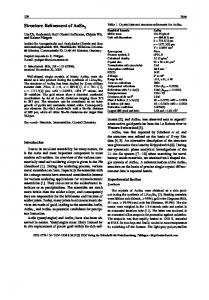
(a) first view

(b) second view

Fig. 1. Merton College. We attempt to adjust this noised reconstruction result and are motivated by the observation that, as illustrated in Fig. 1, there are plenty of planar structures in urban scenes, and many of them are consistent with color coherence and similarity. Though it is not an absolute criterion and many counterexamples may exist, we try to make use of this extra information, which can be effectively extracted from images by performing segmentation. Given a set of images of a scene, we first use structurefrom-motion [8] to compute camera parameter and dense/quasidense method [5, 9, 10] to obtain initial dense/quasi-dense 3D points. Meanwhile, we perform color image segmentation, line detection and matching. With these extra information, we classify the matched feature points into collinear and coplanar grouping sets. Next, we build PCA subspaces for each grouping set of 3D initial points, and find out outlier planes as well as ambiguous points according to eigenvalues and PCA projection distances. Finally, we perform planar adjustment for inlier groups of points and for ambiguous points, we express them in a mixture PCA form and iteratively update them through EM estimation. Finally, non-convergent ambiguous points are eliminated as outliers. To evaluate the proposed method, we carry out experiments on real scene images of open data source (VGG website [11]). Section 2 introduces in detail our structure refinement algorithm. Experimental results are given in Section 3 and the paper is concluded in Section 4.

2953

ICIP 2010

2. PCA-BASED STRUCTURE REFINEMENT

2.1. Building PCA subspaces for Initial Structure

Our structure refinement is essentially a statistical inference process, which estimating the inhomogeneous 3D coordinates of feature points from noised initial structure. Initialization could be performed by different popular methods, in our experiment, we initialize the 3D structure as follows: We first use Bundler Structure from Motion package [12] to compute camera parameters. Then we use quasi-dense [9, 10] method (or PMVS [5] software, refer to section 3) to locate quasi-dense matched feature points and to obtain an initial 3D structure. We then perform color image segmentation using statistical region merging [13]. With the segmentation result and quasi-dense feature points, we select those segments with at least 5 feature points located on and refer to the corresponding 3D points as coplanar points. We also use edge detector to detect line features and match them using MSLD [14]. For each matched line pair, we sample matched point features along them by the method shown in Fig. 2. First uniformly sample point features along the matched line in the first view. Then, for each sampled point, intersect its epipolar line with the matched line in the second view and search for its matched point in the linear neighborhood of the intersection point. We also initialize corresponding 3D points of these matched pairs and refer to them as collinear points. Our structure refinement is designed towards these two kinds of selected 3D points. We denote them as • = {Xn }, n = 1, · · · , N . We then build grouping sets of these points, according to their collinearity or coplanarity. We denote a grouping set by • k , • k ⊂ • , k ⊂ κ, e.g. • 1 = {X5 , X9 , · · · }.κ = {1, · · · , K} is the index set of {• k }, also, κ = κl κp , κl and κp denote index sets of collinear grouping sets and coplanar grouping sets respectively.

(a) first view

By previous stages, we have already obtained initial 3D structure • = {X1 , · · · , XN } and grouping sets • k , k = 1, 2, · · · , K. We then perform principal component analysis (PCA) on each grouping set • k , i.e. equivalently performing SVD on the transformed point matrix of inhomogeneous coordinates. For each group, we get a centroid point  (k) (k) (k) C (k) = |• 1k | Xn , three eigenvalues (λ1 , λ2 , λ3 ) Xn ∈•

k

(supposing descending sorted) and their corresponding eigen(k) (k) (k) vectors (e1 , e2 , e3 ). We can infer structure information of this grouping set from the eigenvalues: For a grouping set of collinear points, λ1 is supposed to be distinctively large, while λ2 and λ3 approximate to zero compared with λ1 . We set a threshold (adaptively selected) for this criterion, to decide whether this grouping set is accepted as an inlier collinear set. For a grouping set of coplanar points, both λ1 and λ2 should be distinctively large and λ3 should approximate to zero. We also set a threshold for this criterion to decide whether this coplanar set obtained from image segmentation is acceptable. We should also consider the degenerate situation here, i.e. λ1 , λ2 , λ3 satisfy the collinear situation, which indicates that this group of points distribute almost linearly on a plane. 2.2. Structure Refinement Once PCA models for all the grouping sets have been built, we can estimate each grouped point by projecting it to its affiliated PCA subspace. Projection of point Xn on the subspace by • k is: 1or2  (k) (k) ˆ (k) = C (k) + αi ei (1) X n i=1

where (k)

αi

(k) T

= ei

(Xn − C (k) )

(2)

with superscript T denoting the matrix transposition. For points of an inlier collinear set, we only calculate the first component of the summary term of Eq.1, i.e. projecting Xn to the best fitting line of • k . For points of an inlier coplanar set, we calculate the first two components of the summary term of Eq.1, i.e. projecting Xn to the best fitting plane of • k. However, for those points with large projection error, this estimation is not reliable, as they may be outliers in the sense of multiple view geometry, or be misleadingly classified to their coplanar sets. We refer to these points as ambiguous points and use a mixture-PCA model to estimate their coordinates or to reject them as outliers:

(b) second view

Fig. 2. Sample point features on matched line pair.

ˆn = X

 k∈κnear

2954

ˆ (k) wn(k) X n

(3)

where κnear ⊆ κ, is the index set of neighboring grouping (k) sets selected for Xn , wn denotes the mixture weight, s.t.  (k) wn = 1. k∈κnear

ˆ n is: Then the parameter set that determine X (k)

(1)

(k)

Θ = (w1 , · · · , wn(k) , · · · , αi , · · · , αi , · · · ) These parameters can be estimated by maximizing the likelihood of Θ given the observed data Xn , without loss of generality, we take the coplanar situation, where the first two eigenvectors are selected, as example:  (k) (k) L(Θ | Xn ) = P (Xn | Θ) = wn(k) Pk (Xn | α1 , α2 ) k∈κnear

(4) (k) ˆ n(k) We refine the mixture weight wn and each projection X (k) (k) (actually α1 , α2 ) of each ambiguous point iteratively, until (k) convergence (i.e. some wn dominates) or over maximum iteration time. Each iteration is based on an EM algorithm for maximizing Eq.4. Details of the EM process left out because of limited space. The detailed deduction is derived from [15], where the update of wnk for each iteration is given by: wn(k)

(k) g

wn 

ˆ g , Θg ) = = P (k | X n

i∈κnear

g

ages we have tested, we choose representative open source images of Merton College (downloaded from VGG website [11], as shown in Fig.1, to show our experimental results. Reasons for doing so is that: First, they are challenging for quasi-dense reconstruction, because there are repeated texture areas and only 3 views of the scene are provided (Fig.1 shows the first two views). Second, other than building blocks with very simple plane structures, the Merton College has a relatively complicated structure, which makes it more challenging and suitable for testing the effectiveness of our algorithm. Our structure refinement method could also be regarded as a filtering process, given the initial 3D structure of matched feature points and the input images. Different quasi-dense reconstruction methods obtain different initial results, however, noise is unavoidable for state-of-art methods, and our refinement can effectively remove some of them. We use two state-of-art methods to produce initial 3D structure, the first is PMVS [5], the second is quasi-dense method based on [9, 10]. Camera parameters is calculated by Bundler package [12]. The image segmentation results are shown in Fig.3

g

ˆ g | α(k) , α(k) ) Pk (X n 1 2 g g g (i) ˆ gn | α(i) , α(i) ) wn Pi (X 1

2

(5) with superscript g denoting the parameter estimated from previous iteration. We select a Gaussian expression of the probabilistic model: 1 ˆ n | α(k) , α(k) ) =  Pk ( X 1 2 (2π)3/2 | k |1/2 (6) −1 1 ˆ (k) T (k) ˆ ˆ ˆ exp{− [(X − X ) ( X − X )]} n n n n k 2 (k)

For the first iteration, the initial value of wn can be set to 1. The iterative refinement algorithm is given in Table. 1

(a) first view

(b) second view

Fig. 3. image segmentation result. As PMVS is a multiple view method, we use all the three images of different views provided by VGG. The point cloud and texture warped results of PMVS reconstruction is shown in Fig.4

Table 1. Iterative structure refinement algorithm (1)

(2)

Step 1. Initialize wn , · · · , wn , · · · = 1 ˆ n | α(k) , α(k) ) by Eq.6 Step 2. For k ∈ κnear , compute Pk (X 1 2 (k)

Step 3. Update each wn by Eq.5 ˆ n by Eq.3 Step 4. Update X (k)

Step 5. Update αi

ˆ n) by Eq.2 (replacingXn withX (a) point cloud

Step 6. If convergent, stop; else, goto Step 2

(b) texture warped result

Fig. 4. PMVS reconstruction result. 3. EXPERIMENTAL RESULTS We have tested our algorithm on a variety of real scene images. However, space lacks for detailed display of all the im-

2955

Noise of the reconstruction result is indistinct by looking at the point cloud, but it is obvious in the texture warped result if looking at some local regions from selected view, as

5. REFERENCES

shown in Fig.5 (a), and the structure refined results are shown in Fig.5 (b) for comparison.

[1] S. Haegler A. Ulmer P. Muller, P. Wonka and L. V. Gool, “Procedural modeling of buildings,” in SIGGRAPH, 2006. [2] P. Tan P. Zhao E. Ofek J. Xiao, T. Fang and L. Quan, “Image-based facade modeling,” in SIGGRAPH Asia, 2008. (a) PMVS results

(b) after structure refinement

Fig. 5. Comparison of local regions. For quasi-dense reconstruction method, we use the two images shown in Fig.1, the reconstruction result is not so good as those by PMVS, as shown in Fig.6. However, after performing the proposed structure refinement, it still obtains an obvious improvement. Comparison results are given in Fig.7

[3] K. Karner L. Zebedin, J. Bauer and H. Bischof, “Fusion of feature- and area-based information for urban buildings modeling from aerial imagery,” in ECCV, 2008. [4] K. Cornelis N. Cornelis, B. Leibe and L. V. Gool, “3d urban scene modeling integrating recognition and reconstruction,” in IJCV, July 2008, vol. 78(2-3), pp. 121– 141. [5] Y. Furukawa and J. Ponce, “http://www.cs.washington.edu/homes/furukawa/research/pmvs,” . [6] G. Vogiatzis C. Hernandez Esteban and R. Cipolla, “Probabilistic visibility for multi-view stereo,” in CVPR, 2007. [7] T. Pock C. Zach and H. Bischof, “A globally optimal algorithm for robust tv-l1 range image integration,” in ICCV, 2007.

(a) point cloud

[8] A Zisserman R Hartley, “Multiple view geometry in computer vision, second edition,” 2003.

(b) texture warped result

Fig. 6. quasi-dense reconstruction result.

[9] M. Lhuillier and L. Quan, “A quasi-dense approach to surface reconstruction from uncalibrated images,” in Pattern Analysis and Machine Intelligence, 2005, vol. 27(3), pp. 418–433. [10] J.Kannala and S S.Brandt, “Quasi-dense wide baseline matching using match propagation,” in CVPR, 2007. [11] Visual Geometry Group @ Oxford “http://www.robots.ox.ac.uk/ vgg/data/,” .

(a) quasi-dense result

(b) after structure refinement

[12] N. Snavely, dler/,” .

University,

“http://phototour.cs.washington.edu/bun-

[13] F Nielsen R Nock, “Statistical region merging,” in Pattern Analysis and Machine Intelligence, 2004.

Fig. 7. Result Comparison.

[14] Z Hu Z Wang, F Wu, “Msld: A robust descriptor for line matching,” in Pattern Recognition, 2008.

4. CONCLUTION In this paper, we propose a new method for refining the 3D structure in reconstruction of urban scenes. This method is essentially a statistical inference process combining both multiple view geometry and color image information. Experiments show that even for state-of-art dense reconstruction results, our refining process attains an improvement.

2956

[15] J.A Bilmes, “A gentle tutorial of the em algorithm an its application to parameter estimation for gaussian mixture and hidden markov models,” in ICSI, 1998, vol. TR-97021,U.C. Berkeley, USA.