Proceedings of the European Control Conference 2007 Kos, Greece, July 2-5, 2007
ThA02.3
PD Control with On-line Gravity Compensation for Robots with Flexible Links Loredana Zollo, Bruno Siciliano, Alessandro De Luca, Eugenio Guglielmelli Abstract— A proportional-derivative (PD) control with online gravity compensation is proposed for regulation tasks of robot manipulators with flexible links. The control law is an extension of a previous PD control with constant gravity compensation at the desired configuration. It is based on a gravity-biased modification of the desired link deflection and requires measuring only position and velocity on the joint side. Global asymptotic stability of the control law at the desired robot configuration is proven via Lyapunov argument and La Salle’s Theorem. Simulation tests on a two-link arm are carried out in order to compare performance of the new scheme with respect to the case of constant gravity compensation and results on the advantages of the on-line compensation are shown. Keywords– Flexible links, PD control
I. INTRODUCTION Introducing flexible elements in robot mechanical structure can be regarded as a useful means to increase the level of safety and more in general dependability of robot manipulators mainly addressed to interaction with humans. Take as an example the application field of biomedical or assistive robotics, where a very close human-robot interaction is a key-element for the robot operating mode and intrinsic compliance is often used to increase robot lightness and safety in the interaction [1], [2], [3], [4]. However, the price to pay is a degradation of robot performance when control algorithms conceived for completely rigid robots are applied to the case of mechanical flexibility [5], [6]. Phenomena of vibrational modes and, in the worst case, instability during interaction [7], [8] may occur. Mechanical flexibility can be thought to be concentrated at joints (in this case robots are referred as robots with elastic joints) or else at links (from here the name of robots with flexible links) [9]. Further, just like for rigid robots, control of flexible robots is aimed at pursuing the two main goals of regulation and tracking control. In this work, attention is focused on the control of robot manipulators with flexible links for regulation to a desired final configuration. In the case of rigid robots, it is well known that global regulation to a desired configuration qd can be achieved by a PD control law, either with a constant gravity compensation L. Zollo and E. Guglielmelli are with Biomedical Robotics and EMC Laboratory, Universit`a Campus Bio-Medico, via Emilio Longoni 83, 00155 Roma, Italy ({l.zollo, e.guglielmelli}@unicampus.it). B. Siciliano is with PRISMA Lab, Dipartimento di Informatica e Sistemistica, Universit`a di Napoli Federico II, via Claudio 21, 80125, Napoli, Italy (
[email protected]). A. De Luca is with Dipartimento di Informatica e Sistemistica, Universit`a di Roma “La Sapienza”, via Eudossiana 18, 00184 Roma, Italy (
[email protected]).
ISBN: 978-960-89028-5-5
term g(qd ) (and sufficiently large positional gains) [10] or with a nonlinear gravity compensation term g(q) evaluated (on-line) at the current configuration [11]. In the case of link flexibility, it has been proven in [12] that a simple PD controller suffices to globally stabilize about any desired configuration flexible arms under gravity. The control stability was demonstrated for the full nonlinear model of multilink flexible robots in presence of constant feedforward gravity compensation, which is evaluated at the desired reference position, and in absence of feedback from the elastic coordinates. The extension to the on-line gravity compensation is complicated by the fact that gravity torque depends on the robot joint coordinates and on the link deflections, whereas quite often only the joint positions are measurable. To this regard, special attention is posed in the literature to the use of observers to estimate link deflection rates [13], [14], [15]. The contribution of this paper is to provide a PD control law with on-line gravity compensation for robot manipulators with flexible links which requires only joint measurements and has guaranteed global stabilization properties. In a way similar to the approach in [16], [4] for robots with elastic joints, the fundamental idea is to use a new variable, named ‘gravity-biased’ modification of the desired deflection, for estimating the gravity torque at each configuration. This controller allows improving the transient behavior of the original control law in [12]. Also, if used in combination with a point-to-point interpolating trajectory, it allows: • operating at lower motor torques by preventing motor saturation (typically occurring during the first instant of motion); • reducing the position error and the oscillations in link deflections and joint torques. The work is organized as follows. Section II recalls dynamic modelling of robot manipulators with flexible links. Section III introduces the PD control law with on-line gravity compensation, the analysis of the closed-loop equilibria and the proof of asymptotic stability via a Lyapunov argument. Finally, simulation results on a two-link flexible arm are reported in Sect. IV. They are compared with the PD control with constant gravity compensation for robots with flexible links. II. DYNAMIC MODEL Consider an n-link flexible arm where bending deformations are limited for each link to the plane of rigid motion. Under the following assumptions [9]:
4365
ThA02.3 A1. the arm is a slender beam with uniform geometric characteristics and homogeneous mass distribution; A2. the arm is flexible in the lateral direction, being stiff with respect to axial forces, torsion, and bending forces due to gravity; further, only elastic deformations are present; A3. nonlinear deformations as well as internal friction or other external disturbances are negligible effects; the closed-form dynamic equations of the arm can be written as µ ¶ µ ¶ 0 u H(q)¨ q + c(q, q) ˙ + g(q) + = (1) 0 Dδ˙ + Kδ ¡ ¢T being q = θT δ T , with θ the (n × 1) vector of joint coordinates and δ the (m × 1) vector of link coordinates of an assumed mode description of link deflections. Equation (1) can be rewritten more explicitly as µ
¶µ ¶ µ ¶ ˙ δ) ˙ Hθθ (θ, δ) Hθδ (θ, δ) θ¨ cθ (θ, δ, θ, + T ˙ δ) ˙ Hθδ (θ, δ) Hδδ (θ, δ) cδ (θ, δ, θ, δ¨ µ ¶ µ ¶ µ ¶ 0 gθ (θ, δ) u + + = . (2) gδ (θ, δ) 0 Dδ˙ + Kδ
In (2) the ((n + m) × (n + m)) positive definite symmetric inertia matrix H has been partitioned in blocks according to the rigid and flexible components, c is the ((n ´ × 1) ³ + m) ∂U vector of Coriolis and centrifugal forces, g = ∂qg is the ((n + m) × 1) vector of gravitational forces, being Ug the potential energy due to gravity. Further, K and D are the system stiffness and damping diagonal matrices. It is worth noticing that three important properties hold, which play an important role in demonstrating control stability. They are: P1. It can be shown (as for the rigid case) that a factorization of c exists c(q, q) ˙ = S(q, q) ˙ q˙ such that¡ H˙ − 2S¢ is skew-symmetric. P2. Let Ue = 21 δ T Kδ denote the elastic energy stored in the links. Condition Ue ≤ Uemax < ∞ leads to
s
2Uemax kδk ≤ . (3) λmin (K) P3. The vector of gravitational torques can be partitioned as ¶ µ gθ (θ, δ) g(q) = gδ (θ)
where the dependence of gδ only on θ is due to the assumption of small deformation of each link. For it, the following inequalities hold: s ° ° ° ∂g ° ° °≤ α0 + α1 kδk≤ α0 + α1 2Uemax =: α (4) ° ∂q ° λmin (K)
kg(q1 ) − g(q2 )k ≤ α kq1 − q2 k .
(5)
with α0 , α1 , α > 0. III. PD CONTROL LAW In this section, a control law is proposed which is aimed at regulating to a desired constant configuration ¡ robot ¢position T by means of a proportional-derivative qd = θdT δdT action in the space of joint variables and a sort of on-line compensation of the gravitational torque at any configuration during motion. The on-line gravity compensation has the main purpose of improving robot performance during regulation tasks. Thus, the control in [12] is resumed, under the same hypothesis that only the joint variables are measurable, and is extended to the case of an on-line gravity compensation. The PD control with constant gravity compensation in [12] is expressed as u = KP (θd − θ) − KD θ˙ + gθ (θd , δd ),
(6)
where KP and KD are (n × n) symmetric positive definite matrices and δd = −K −1 gδ (θd ).
(7)
Global asymptotic stability of the (unique) closed-loop equilibrium state q = qd , q˙ = 0 was proven under the assumption that λmin (Kq ) = λmin
µ
Kp 0
0 K
>α
(8)
with α as in (4). On the other hand, the PD control law with on-line gravity compensation is formulated as follows: ˜ u = KP (θd − θ) − KD θ˙ + gθ (θ, δ),
(9)
where δ˜ is a ‘gravity-biased’ modification of the desired deformation δd expressed as: ¡ ¢ δ˜ = − δd + 2K −1 gδ (θ)
(10)
It should provide the correct gravity compensation at steady state, even without a direct measure of δ. As a matter of fact, the control law (9) can be implemented using only joint variables. A. Closed-loop equilibria The equilibrium configurations of the closed-loop system (1), (9) are computed by setting θ˙ ≡ δ˙ ≡ 0. This yields
4366
˜ gθ (θ, δ) = KP (θd − θ) + gθ (θ, δ)
(11)
gδ (θ) = −Kδ.
(12)
ThA02.3 The following expansion holds true: ˜ − gθ (θd , δ˜d ) = gθ (θ, δ) ˜ − gθ (θd , δd ) = gθ (θd , δd ) gθ (θ, δ) ¯ ¯ ˜ ¯ ∂gθ (θ, δ) (˜ q − q˜d ) + o(k˜ q − q˜d k2 ) − gθ (θd , δ˜d ) + ¯ ∂ q˜ ¯ θ=θd ,δ=δd ¶ µ ´¯ ³ θ − θd ˜ ˜ ¯ (θ,δ) ∂gθ (θ,δ) = gθ (θd , δd ) + ∂gθ∂θ ¯ ˜ − δ˜d ∂ δ˜ θ=θd ,δ=δd δ
+o(k˜ q − q˜d k2 )−gθ (θd , δd ) ³ ´¯ ˜ ˜ ¯ (θ,δ) ∂gθ (θ,δ) = ∂gθ∂θ ¯ ˜ ∂δ
θ=θd ,δ=δd
2
µ
θ − θd δ˜ − δ˜d
+o(k˜ q − q˜d k ) ¢T ¡ being q˜ = θT δ˜T From (11) and (13) it follows that
(13)
° °2 2 2 ≤ α2 kqd − qk + α♯2 kθd − θk + °o(k˜ q − q˜d k2 )° 2
2
2
= α2 kθd − θk + α2 kδd − δk + α♯2 kθd − θk ° °2 ¡ ¢ 2 + °o(k˜ q − q˜d k2 )° = α2 + α♯2 kθd − θk ° °2 2 +α2 kδd − δk + °o(k˜ q − q˜d k2 )° ,
(19)
with α♯ to be defined below. It has to be noted that in (19) the following inequalities have been used: °Ã !°2 ° ° ° ° ° ∂gθ (θ,δ) ° ° ∂g (θ, δ) ° °2 ° ∂gδ (θ) °2 ° ∂g(q) °2 ° ° ° θ ° ∂q ° =° ° +° ° ° = ° ∂gδ (θ) ° ∂q ° ° ° ∂q ° ° ∂q ° ° ∂q ≤
2
∗ ∗2 (α01 + α1 kδk) + α02
(20)
˜ gθ (θ, δ)=KP (θd − θ)+gθ (θ, δ)+g θ (θd , δd )−gθ (θd , δd ) ¯ ¯ ˜ ∂gθ (θ, δ) ¯ (˜ q − q˜d )+gθ (θd , δd ) = KP (θd − θ)+ ¯ ∂ q˜ ¯
s ° ° ° ∂gθ (θ, δ) ° 2Umax ∗ ∗ ∗ ° ° ° ∂q ° ≤ α01 +α1 kδk ≤ α01 +α1 λmin (K) = α1 (21)
and the closed-loop system (11), (12) becomes
and, consequently,
θ=θd ,δ=δd
+o(k˜ q − q˜d k2 )
° ° ° ∂gδ (θ) ° ∗ ∗ ° ° ° ∂q ° ≤ α02 = α2 .
(14)
KP (θd − θ) = gθ (θ, δ) − gθ (θd , δd ) ¯ ˜ ¯¯ ∂gθ (θ, δ) (˜ q − q˜d ) − o(k˜ q − q˜d k2 ) − ¯ ∂ q˜ ¯
(15)
(22)
kgθ (q1 ) − gθ (q2 )k ≤ α1∗ kq1 − q2 k
(23)
kgδ (θ1 ) − gδ (θ2 )k ≤ α2∗ kθ1 − θ2 k
(24)
θ=θd ,δ=δd
K(δd − δ) = gδ (θ) − gδ (θd ).
and
(16)
where condition (7) has been used. Equations (15), (16) can be written as
° °2 ¯¯ ° ∂g (θ, δ) ° ¯ ˜ ° θ ° ¯ 2 2 k˜ qd − q˜k ≤ α1∗2 k˜ qd − q˜k ° ° ° ∂ q˜ ° ¯¯ θ=θd ,δ=δd ³ ° °2 ´ 2 ∗2 = α1 kθd − θk + °2K −1 (gδ (θd ) − gδ (θ))° ° °2 2 2 ≤ α1∗2 kθd − θk + α1∗2 °2K −1 ° kgδ (θd ) − gδ (θ)k ° °2 2 2 ≤ α1∗2 kθd − θk + α1∗2 α2∗2 °2K −1 ° kθd − θk ³ ´ ° °2 2 = α1∗2 kθd − θk 1 + α2∗2 °2K −1 ° ¡ ¡ ¢¢ 2 ≤ α1∗2 1+α2∗2 λ2max 2K −1 kθd − θk
Kq (qd − q) = g(q) − g(qd ) ¯ Ã ! ˜ ¯ ∂gθ (θ,δ) (˜ q − q˜d ) + o(k˜ q − q˜d k2 ) ¯ ∂ q ˜ − (17) θ=θd ,δ=δd 0
being
Kq =
µ
Kp 0
0 K
.
Taking into account conditions (4), (5), the following inequalities can be derived, if assumption (8) holds true: kKq (qd − q)k ≥ λmin (Kq ) kqd − qk > α kqd − qk ≥ kg(qd ) − g(q)k
(25)
∗ with α1∗ , α01 , α2∗ , α♯ > 0. From (18) it follows that
(18)
and ¯ ° !°2 à ˜ ¯ ∂gθ (θ,δ) ° (˜ q − q˜d )+o(k˜ q − q˜d k2 ) ° ¯ ° ° ∂ q ˜ θ=θd ,δ=δd ° °g(q)−g(qd )− ° ° 0 ° ° ¯ ° °2 ˜ ¯¯ ° ∂gθ (θ, δ) ° 2 ° (˜ q − q˜d )° = kg(qd ) − g(q)k + ° ¯ ° ∂ q˜ ¯ ° ° θ=θd ,δ=δd ° ° 2 2 + °o(k˜ q − q˜d k2 )° ≤ α2 kqd − qk ¯ °2 ¯ ° ° ° ∂g (θ, δ) ° °2 ° θ ˜ ° ¯¯ 2 k˜ qd − q˜k + °o(k˜ q − q˜d k2 )° +° ° ¯ ° ∂ q˜ ° ¯ θ=θd ,δ=δd
2
= α♯2 kθd − θk .
2
2
2 kKq (qd − q)k ≥ Kqm kqd − qk
2
2
2 2 = Kqm kθd − θk +Kqm kδd − δk
(26) 2
being Kqm = λmin (Kq ). Thus, neglecting o(k˜ q − q˜d k ), equality (17) holds true only for (θ, δ) = (θd , δd ) under the assumption that ¡ ¢ 2 > α2 + α♯2 Kqm (27)
is satisfied. Summarizing, locally around (θ, δ) = (θd , δd ), (θd , δd ) is a unique isolated equilibrium configuration of the closed-loop system (1), (9).
4367
ThA02.3 B. Proof of asymptotic stability The stability of the proposed control law is proven by using the direct Lyapunov method and then invoking LaSalle’s Theorem. Consider the auxiliary configuration-dependent function P (q, q˜) = P (θ, δ) = + Ug (q) − Uθ (˜ q ).
1 1 T T δ Kδ + (θd − θ) KP (θd − θ) 2 2 (28)
where Ug is the potential energy due to gravity such that ∂Ug (q) = ∂q
µ
gθ (θ, δ) gδ (θ)
and Uθ is defined as Uθ (˜ q) =
R
∂Ug (˜ q) ∂θ dθ
(29)
˜ −θ˙T KP (θd − θ) − θ˙T gθ (θ, δ) T T = −θ˙ KD θ˙ − δ˙ Dδ˙ ≤ 0 (30)
It is easy to see that this function, under assumption (27), has a unique minimum in (θd , δd ). In fact, the necessary condition for a minimum of P (q, q˜) is ∇θ P ∇δ P
¸
∇P (q, q˜) = · ¸ ˜ −KP (θd − θ) + gθ (θ, δ) − gθ (θ, δ) = = 0. (31) Kδ + gδ (θ) Equation (31) is exactly in the form (11), (12). Using the same arguments of Section III-A, it can be obtained that ∇P (q, θ) = 0 only at (θd , δd ). Moreover, 2
·
∇2θ P ∇δ ∇θ P
¸¯ ¯ ¯ ¯ θ=θd ,δ=δd #¯ ¯ ∂gδ (θ) ¯ ∂θ ¯ ¯ K θ=θ ,δ=δ
∇θ ∇δ P ∇2δ P
∇ P (θd , δd ) = " ˜ (θ,δ) (θ,δ) KP + ∂gθ∂θ − ∂gθ∂θ = ˜ (θ,δ) ∂gθ (θ,δ) − ∂gθ∂δ ∂δ ¸ · (θd ) KP ∂gδ∂θ . = 0 K
˜ = θ˙T KP (θd − θ) −θ˙T KP (θd − θ)+ q˙T g(q) − θ˙T gθ (θ, δ) ˜ − δ˙ T Dδ˙ − δ˙ T Kδ + δ˙ T Kδ −θ˙T KD θ˙ + θ˙T gθ (θ, δ)
such that
∂Uθ (˜ q) = gθ (˜ q ). ∂θ
·
Along the trajectories of the closed-loop system (1), (9), the time derivative of V becomes 1 ˙ q˙ + δ˙ T Kδ − θ˙T KP (θd − θ) V˙ = q˙T H(q)¨ q + q˙T H(q) 2 µ ¶T µ ¶T q) T ∂Ug (q) T ∂Uθ (˜ ˙ + q˙ −θ = q˙T (−c(q, q) ˙ − g(q)) ∂q ∂θ ¶¶ µ µ ¶ µ 1 0 u ˙ q˙ + δ˙ T Kδ + q˙T H(q) + − + 0 Dδ˙ + Kδ 2 ˜ = −q˙T g(q) −θ˙T KP (θd − θ) + q˙T g(q) − θ˙T gθ (θ, δ) ! à ˜ KP (θd − θ) − KD θ˙ +´ gθ (θ, δ) ³ T +q˙ + δ˙ T Kδ − Dδ˙ + Kδ
d
d
(32)
The sufficient condition for a minimum, i.e. ∇2 P (θ, δ)|θ=θd ,δ=δd > 0.
(33)
is satisfied under the assumption (8). The function derived from (28) as ˙ δ) ˙ = 1 q˙T H(q)q˙ + P (θ, δ) − P (θd , δd ) V (θ, δ, θ, 2 is zero at the chosen equilibrium state, θ = θd , δ = δd , θ˙ = δ˙ = 0, and positive for any other state in an open neighborhood of this equilibrium, provided that condition (27) holds true. Hence, V is a candidate Lyapunov function.
(34)
where the skew-symmetry of matrix H˙ − 2S as appears in Property P1. has been used. When V˙ = 0, it is θ˙ = δ˙ = 0 and the closed-loop equations give ˜ gθ (θ, δ) = KP (θd − θ) + gθ (θ, δ) gδ (θ) = −Kδ.
(35) (36)
In view of the previous equilibrium analysis and of condition (27), it is q¨ = 0 if and only if q = qd , or θ = θd and δ = δd . Invoking LaSalle’s invariant set Theorem, asymptotic stability of the desired point follows. IV. SIMULATION RESULTS Simulation tests have been carried out in order to measure dynamic performance of the PD controller with on-line vs. constant gravity compensation. To this purpose, the planar two-link flexible arm under gravity shown in Fig. 1 is modeled. Robot dynamics as well as the regulation task are the same as those reported in [12]. The arm has the initial vertical equilibrium configuration θi = [ −π/2 0 ]T rad, δi = [ 0 0 0 0 ]T m and is commanded to reach the desired configuration θd = [ −π/4 0 ]T rad, δd = [ −0.15 −0.0045 −0.0056 −0.000076 ]T m. The task is repeated for the two cases of constant gravity compensation (i.e. control law (6)) and on-line gravity compensation (i.e. control law (9)) and results are reported in Figs. 2-3 and Figs. 4-5, respectively. Although both controllers achieve the correct steady-state position, the transient with the on-line gravity compensation is smoother than that with the constant gravity compensation and link deformations and motor torques are visibly reduced (Figs. 3, 5). It has to be noted that simulation tests have been carried out with the same PD feedback gains KP = diag{15, 15} Nm/rad and KD = diag{3, 3} Nms/rad. Improvements due to on-line gravity compensation are particularly evident when the control is applied to the case of a desired variable reference position over time instead of
4368
ThA02.3 link deflections δ2
0
joint torques 20
δ4
15
δ3
[Nm]
[m]
−0.05 δ1
−0.1 −0.15
10
link 1
5
link 2
0
−0.2 0
2
4
−5 0
6
2
time [s]
4
6
time [s]
Fig. 5. Link positions and motor torques with on-line gravity compensation for constant reference A planar two-link flexible arm
joint position error
joint angles 1 link 2
0.4 0.2 0
[rad]
[rad]
0.6 link 1
link 1
−1 link 2
−0.2 0
0
2
4
−2 0
6
2
time [s]
4
6
time [s]
Fig. 2. Joint position error and joint angles with constant gravity compensation for constant reference
link deflections δ2
0
15 [Nm]
δ3
−0.05 [m]
joint torques 20
δ4
δ1
−0.1 −0.15 −0.2 0
10
link 1
5
link 2
0 2
4
−5 0
6
2
time [s]
4
a constant configuration. This choice is motivated by the fact that the big initial error inevitably present in a regulation to a constant reference position can be cause of motor saturation and large torque values. Using a variable position reference can overcome this critical issue. A point-to-point quintic polynomial trajectory (with zero velocity and acceleration boundary conditions) has been T planned from the initial configuration qi = ( θiT δiT ) T up to the final configuration qd = ( θdT δdT ) in a time interval of 4 s, with 2 s for the adjustment. Due to the initial null error, both controllers (6) and (9) can perform the motion with sufficiently high positional gains KP = diag{1000, 1000} Nm/rad. The results are shown in Figs. 6 and 7 for constant gravity compensation and, respectively, in Figs. 8–9 for online gravity compensation. A comparison of Fig. 6 with Fig. 8 indicates a reduction of the overall positional error obtained thanks to on-line gravity compensation. Also, the torque profile is different; in particular at the initial time instants, a ripple is present for the case of constant gravity compensation (Figs. 7 and 9). Ripple is still present even if the control gains are changed, although the results are not presented here for brevity.
6
time [s]
−3
5
x 10
joint angles
joint position error 0.5
link 2
Fig. 3. Link positions and motor torques with constant gravity compensation for constant reference [rad]
0 −5
0
link 2
[rad]
Fig. 1.
link 1
−10
joint position error
−15 0
joint angles 1
link 1
0
link 2
[rad]
[rad]
0.2
−1.5 2
4
6
−2 0
2
4
6
time [s]
Fig. 6. Joint position error and joint angles with constant gravity compensation for polynomial trajectory
link 1
−1
−0.2 0
link 2
0
link 1
−1
time [s]
0.6 0.4
−0.5
2
4 time [s]
6
−2 0
V. CONCLUSIONS 2
4
6
time [s]
Fig. 4. Joint position error and joint angles with on-line gravity compensation for constant reference
This paper has proposed a PD control action on the joint variables with on-line gravity compensation for flexible link manipulators. The novelty of the control with respect to the previous work in [12] is the estimate of gravity torque in a gravity-biased modification of the desired link deformation
4369
ThA02.3
δ3
[Nm]
[m]
−0.05 δ1
−0.1 −0.15
link deflections
4
2
4
−4 0
6
link 2
2
−3
4
6
[rad]
[rad]
link 2
[7]
−0.5
link 1
−1
[8]
−1.5 4
2 0
link 2
2
4
6
−4 0
2
4
6
time [s]
Fig. 9. Link positions and motor torques with on-line gravity compensation for polynomial trajectory
link 2
0
link 1
2
4
−2 time [s]
0.5
1
−1 0
link 1
joint angles
joint position error
0
δ1
−0.1
−0.2 0
time [s]
Fig. 7. Link positions and motor torques with constant gravity compensation for polynomial trajectory
x 10
4
δ3
−0.15
time [s]
2
joint torques 8 6
δ
−0.05
2 0 −2
−0.2 0
δ2
0
link 1
[m]
δ2
0
joint torques 8 6
δ4
[Nm]
link deflections
6
−2 0
time [s]
2
4
6
[9]
time [s]
[10] Fig. 8. Joint position error and joint angles with on-line gravity compensation for polynomial trajectory [11]
δd based on joint variables, in lieu of the actual link deflection. This avoids the use of extra sensors on the link side for measuring link deflections. Global asymptotic stability of this control law has been proven through a Lyapunov argument and La Salle’s Theorem. Control performance has been evaluated by means of simulations tests on a twolink arm with flexible links. The results have shown that the proposed controller with on-line gravity compensation typically outperforms the previous controller with constant gravity compensation in terms of transient behavior and torque values. This has been studied for the case of constant reference position and for the case of an interpolating reference trajectory for regulation tasks, in order to avoid the problem of actuator saturation.
[12] [13] [14] [15] [16]
R EFERENCES [1] K. Kiguchi, K. Iwami, M. Yasuda, K. Watanabe, “An exoskeletal robot for human shoulder joint motion assist”, IEEE/ASME Trans. on Mechatronics, vol. 8, pp. 125–135, 2003. [2] D.J. Reinkensmeyer, L.E. Kahn, M. Averbuch, A. McKenna-Cole, B.D. Schmit, W.Z. Rymer, “Understanding and treating arm movement impairment after chronic brain injury: Progress with the ARM guide”, J. of Rehabilitation Research and Development, vol. 37, pp. 653–662, 2000. [3] L. Zollo, B. Siciliano, C. Laschi, G. Teti, G., P. Dario, “An experimental study on compliance control for a redundant personal robot arm”, Robotics and Autonomous Systems, vol. 44, pp. 101–129, 2003. [4] L. Zollo, B. Siciliano, A. De Luca, E. Guglielmelli, P. Dario, “Compliance control for an anthropomorphic robot with elastic joints: Theory and experiments”, ASME J. of Dynamic Systems, Measurements, and Control, vol. 127, pp. 321–328, 2005. [5] E.I. Rivin, “Effective rigidity of robot structure: Analysis and enhancement”, American Control Conference, Boston, MA, 1985. [6] L.M. Sweet, M.C. Good, “Re-definition of the robot motion control problem: Effects of plant dynamics, drive system constraints, and user
4370
requirements”, 23rd IEEE Conference on Decision and Control,Las Vegas, NV, pp. 724–731, 1984. M.W. Spong, “On the force control problem for flexible joint manipulators”, IEEE Transactions on Automatic Control, vol. 34, pp. 107–111, 1989. R.K. Roberts, R.P. Paul, B.M. Hilberry, “The effect of wrist sensor stiffness on the control of robot manipulators”, IEEE International Conference on Robotics and Automation, St. Louis, MO, pp. 269–274, 1985. C. Canudas de Wit, B. Siciliano, G. Bastin, (Eds.), Theory of Robot Control, Springer-Verlag, London, UK, 1996. S. Arimoto, F. Miyazaki, “Stability and robustness of PID feedback control for robot manipulators of sensory capability”, Robotics Research: 1st Int. Symp., Brady, M., and Paul, R. P. (Eds.), Cambridge, MIT Press, pp. 783–789, 1984. L. Sciavicco, B. Siciliano, Modelling and Control of Robot Manipulators, (2nd Ed.) London, Springer, 2000. A. De Luca, B. Siciliano, “Regulation of flexible arms under gravity”, IEEE Transactions on Robotics and Automation, vol. 9, pp. 463–467, 1993. M.A. Arteaga, “Position determination for flexible robot arms”, Research Report (in German), No. 9/95, Department of Measurement and Control, University of Duisburg, Germany, 1995. M.A. Arteaga, B. Siciliano, “Tracking control of flexible robot arms”, IEEE Transactions on Automatic Control, vol. 45, pp. 520–527, 2000. M.A. Arteaga, “Tracking control of flexible robot arms with nonlinear observer”, Automatica, vol. 36, pp. 1329–1337, 2000. A. De Luca, B. Siciliano, L. Zollo, “PD Control with on-line gravity compensation for robots with elastic joints: Theory and experiments”, Automatica, vol. 41, pp. 1809–1819, 2005.