A HYBRID FINITE VOLUME/PDF MONTE CARLO METHOD TO CAPTURE SHARP GRADIENTS IN UNSTRUCTURED GRIDS Genong Li and Michael F. Modest Mechanical Engineering Department The Pennsylvania State University University Park, PA 16802 Email:
[email protected]
ABSTRACT The hybrid finite volume/PDF Monte Carlo method has both the advantages of the finite volume method’s efficiency in solving flow fields and the PDF method’s exactness in dealing with chemical reactions. It is, therefore, increasingly used in turbulent reactive flow calculations. In order to resolve the sharp gradients of flow velocities and/or scalars, fine grids or unstructured solution -adaptive grids have to be used in the finite volume code. As a result, the calculation domain is covered by a grid system with very large variations in cell size. Such grids present a challenge for a combined PDF/Monte Carlo code. To date, PDF calculations have generally been carried out with large cells, which assure that each cell has a statistically meaningful number of particles. Smaller cells would lead to smaller numbers of particles and correspondingly larger statistical errors. In this paper, a particle tracing scheme with adaptive time step and particle splitting and combination is developed, which allows the PDF/Monte Carlo code to use any grid that is constructed in the finite volume code. This relaxation of restrictions on the grid makes it possible to couple PDF/Monte Carlo methods to all popular commercial CFD codes and, consequently, extend existing CFD codes’ capability to simulate turbulent reactive flow in a more accurate way. To illustrate the solution procedure, a PDF/ Monte Carlo code is combined with FLUENT to solve a turbulent diffusion combustion problem in an axisymmetric channel.
INTRODUCTION
It is well known that PDF/Monte Carlo method can treat chemical reactions and other nonlinear interactions more accurately and with relative ease (Pope Ref. [1]). In hybrid numerical methods, the flow field (including velocities, pressure, turbulent kinetic energy and the dissipation rate of turbulent kinetic energy) is solved by finite volume techniques, while scalars such as mass fraction of species and temperature are solved by composition PDF/Monte Carlo techniques. The hybrid methods combine both the advantages of the finite difference method’s efficiency in solving the flow field and the PDF method’s exactness in dealing
with chemical reactions. It is, therefore, increasingly used in turbulent reactive flow calculations. In the PDF/Monte Carlo simulation, a large number of particles is employed to represent the real flow fields. Mean values of scalars are calculated by averaging over many Lagrangian particles. The method requires a sufficient number of particles to be in each cell at all times to keep statistical noise low to ensure reliable mean values. The number of particles employed in a simulation has a first-order effect on the overall cost of the calculation. A uniform number of particles per computational cell throughout the flow domain ensures that computational effort is used efficiently; however, this optimal situation is not attained in most situations. As pointed out by Li and Modest [2], the use of cells with large variations in size is the major cause of unbalanced number of particles in different computational cells in incompressible flows. In addition, density variations can also cause cell populations to become unbalanced since, if equal mass particles are used, low density regions tend to have less particles in a cell. This imbalance problem is particularly severe in axisymmetric systems, in which cells near the axis tend to suffer from low particle counts due to their small volume and scalars are difficult to resolve accurately, while outside cells tend to hold too many particles and thus wastes computer resources. In many such flows, sharp gradients of the flow field occur near the axis where even smaller cells are required to be used, which makes things even worse. Similar problems have been recognized in other types of Monte Carlo simulations. For instance, in direct Monte Carlo simulations of rarefied and nonequilibrium gas flows or in the simulation of plasma, the imbalance of particle counts has also been recognized as a problem. Kannenberg and Boyd [3] discussed three possible ways to overcome it: direct variation of particle weights, variation of time steps and grid manipulation. Lapenta [4] used particle splitting and coalescing (combination)
to control the number of particles per cell in his plasma simulation. All these techniques have been used in PDF/Monte Carlo simulations although in a slightly different interpretation. In the field of PDF/Monte Carlo simulation, Li and Modest [2] proposed a particle tracing scheme with adaptive timestep splitting and particle splitting and combination procedure, which can overcome the problem of unbalanced numbers of particles in different cells and can improve the computational efficiency. They showed strong improvement in numerical performance of the new scheme by applying it to a simple planar diffusion problem. In that paper, the variation of cell size is only about 13:1 and no chemical reactions are considered. Thus, a more severe test is needed to demonstrate the new method’s validity in turbulent reactive flows. This study is a further step in the development of a comprehensive hybrid model for turbulent reactive flows with thermal radiation effects. To capture the strong gradients in such flows, a locally clustered mesh or even an adaptive mesh has to be used in the finite volume solver. Unstructured grids not only provide greater flexibility in discretizing complex domains but also enable straightforward implementation of adaptive meshing techniques where mesh points may be added or deleted locally (Mavriplis Ref. [5]). Many finite volume codes, such as FLUENT [6], allow the use of such unstructured meshes. To accommodate this capability, particle tracing needs to be adapted to unstructured meshes. In this paper, a so-called element-to-element particle tracing strategy for unstructured meshes is presented, which is very efficient when used with the timestep splitting procedure. The particle splitting and combination procedure is discussed in more depth in this paper, the possible side effects of splitting and combining on the stochastic system and the requirements of preserving mean quantities such as mass, scalars or moments of scalars will be investigated. In the following we first describe our element-to-element particle tracing method in a triangular mesh; then we review the adaptive timestep splitting and mean estimation in the framework of unstructured meshes. The particle splitting and combination process is investigated next, followed by a static test. Finally, a turbulent reactive flow in an axisymmetric channel is solved to demonstrate the performance of the method.
PARTICLE TRACING IN TRIANGULAR MESHES
In PDF/Monte Carlo solvers, every particle changes its position in the computational domain during each time step and the host cell for it needs to be traced. There are many possible strategies (Lohner Ref. [7]) for doing that. The use of successive neighbor searches turns out to be the most suitable method considering the fact that particles most likely stay in the same cell or simply move to one of their neighboring cells after a single time step, which is especially true in the calculation here because of the use of an adaptive time step splitting technique.
(i)
(j)
V2 (V1 ) h(j)1 n
(i) 1
(j)
h(i)2 (h(j)3)
n(i)2
n
(i) 1
(i)
V2
cell j
(j) 3
h
n(j)1
O1 h(i)3
n(j)2
O2 cell i (i)
V1
n(i)3
(j) 2
h
(j)
V3 (V3 )
Figure 1. Illustration of particle tracing in triangular cells
Assume a particle resides in cell with position 1 originally and moves to 2 after one time step. To identify its new host cell, first three quantities are calculated,
1
2 () 1
() 1
;
1
2 () 2
() 2
;
1
2 () 3
() 3
where 1( ) , 2( ) and 3( ) are three normal vectors; 1( ) , 2( ) and (3 ) are the shortest distances from point 1 to the three surfaces of cell (see Fig. 1), and the superscript ( ) is used to denote the quantities’ association with cell . If all three quantities are less than unity the particle is still in cell ; if their maximum is greater than unity, this implies that the particle leaves of the cell through the surface on which the maximum is computed. For example, in the case shown in Fig. 1, the second of the above quantities is the largest and the particle leaves the cell through surface 2. The connectivity information of the mesh gives the cell number next to that surface, in this case, . The cell pointer for the particle is updated to that of the neighboring cell, and the above three quantities are recalculated with respect to cell . This process is repeated until the new host cell is found, i. e. , when all three values are less then unity. We call this strategy an element-to-element search. In Subramaniam and Haworth’s paper [8], a face-to-face search strategy is used, in which the time fraction spent in each cell is tabulated. Such information is needed if a cell-center-based PDF code is used (the field means are stored at the centroid of the cells) and one wants to distribute a particle’s contribution to all the cells it passes through according to its residence time in each cell. As will be seen later, in the vertex-based scheme with time step splitting procedure that is used in our current method (the field means are stored at vertices of the cells), the element-to-element search scheme is more efficient.
ADAPTIVE TIME STEP SPLITTING AND MEAN ESTIMATION METHOD
In the PDF/MC method, scalar fields need to be updated on an Eulerian finite volume grid using information from Lagrangian particles, which carry mass as well as scalar information. There are many ways to calculate field means from the particles’ properties. The simplest way is to tally particles only at the end of a whole time step. Field means of a cell can be calculated as simple averages of the properties of all particles in a cell or the means can be computed by weighted-avarging of the properties of its surrounding particles, in which the weight is determined by some linear-basis functions. Weighted-averaging leads to less variance and is widely used in PDF/Monte Carlo methods today. The above methods only tally particles at the end of one entire time step. As discussed in our previous paper (Li and Modest Ref. [2]), if cells with large variation in size are used, the time step is limited by the time scale of the smallest cell in the flow field making particle tracing very inefficient. If a large time step is taken, a particle may pass through several cells in a single time step. As a result, this not only tends to smoothen the flow field but also leads to bad statistics since a particle may pass through several cells without leaving any contribution to them. To overcome this shortcoming, an adaptive time-step is used, in which a global time step is determined by the largest cell time scale, which is then split into sub-steps, if necessary, according to the particle’s position. Here, a time step is split such that a particle changes its location neither too little nor too much in a single move, by comparing the move to the cell size in which the particle resides. In the context of an unstructured triangular mesh, the particle’s stochastic differential equations (SDEs) are integrated forward in each sub-step and a particle experiences a series of moves in one global time step as shown in Fig. 2. For a particle in cell after the ( 1)th move at some time level, the sub-step for the th move is computed as, = min
(1)
where are the maximum span of cell in the and directions, and , , are the turbulent kinetic energy, its dissipation rate, and two velocity components at the centroid of the cell , respectively. After setting the partial time step, a set of SDEs for particle needs to be integrated. Predictor/corrector (P/C) scheme is used in the integration to achieve better time accuracy. In the composition PDF method, a particle’s location and its properties evolve according to (Subramaniam and Haworth Ref. [8]),
where variables with an asterisk refer to the Lagrangian particle’s properties, and is the turbulent time scale calculated as ; 1 2 = is the turbulent diffisivity, where , and are turbulent Schmidt or Prandtl number and a model constant. is an isotropic vector Wiener process. In equation (3) Dopazo’s is another model scalar mixing model has been used where constant. Finally, is a source term due to chemical reactions. vertices of elements (nodal points) dependence region of V
V2
V
( ) = [( ( )=
+
] 1 2
(
()
+ [2 )
1
]
D
A
V1
V3
X
particle’s path Cell i three influence nodes of any particle in cell i
Figure 2.
The unstructured mesh used in the hybrid FV/PDF method
The predictor step determines the particle’s approximate location after the integration, with the explicit form, +1
1
=
+ [(
+
]
+ [2
]2
(4)
and +1 = superscripts and + 1 denote values at time + , respectively, and is a standardized Gaussian random vector (components with zero mean and unity variance). All mean quantities appearing in the coefficients are evaluated at the as indicated by the subscript. In particle’s initial position our calculations, all mean values are stored at the vertices of the triangular mesh. The field means at arbitrary particle position are linearly interpolated from the three vertex quantities of its host cell: if denotes any mean quantity stored at vertices, the corresponding value at an arbitrary point is, =
1
1
+
2
2
+
3
(5)
3
where 1 , 2 and 3 are the mean quantities at the three vertices, and the weight factors are calculated from a linear basis function. If we confine our discussion to 2D triangular meshes, these are, =
2 3 2 1 2 3
()
O
C
1 1 2
Y
B
=
1 3 3
=
1 2 3
1 2
(6)
1 2 3
(2) (3)
where 1 2 3 , etc., are the area of triangle triangles as shown in Fig. 2.
1 2 3
and its sub-
In the corrector step, all coefficients involving the field means are evaluated as the average of their mean values at the initial and at the predicted location. The corrector step has the form, +1
=
+
1 [ 2
1 [ 2
+1
=
+
]
+[
1
+
]
+
+1
1
]2 + [
]2
+ 2
+
(7)
+1
+1
+
+1
(8) Note that the same value of is used for both predictor and corrector steps, but that different and independent values of are used for each subtime step. It has been verified that this P/C scheme is equivalent to the Runge-Kutta form of Milischtein’s general second-order weak scheme for stochastic systems (Welton Ref. [9]). The mean quantities at nodes are calculated from all particles in a region (dependence region) bounded by surrounding nodes. They are updated at the end of each global time step using, both, the particles properties at the final position as well as those at intermediate positions. The contribution of each sub-move is weighted by its time fraction, so the mean field of scalars can be calculated as
PARTICLE SPLITTING AND COMBINING PROCEDURE
In order to achieve a uniform statistical uncertainty level throughout the computational domain, it is important to have well-balanced numbers of particles residing at all times in each computational cell (which may vary vastly in size). A particle splitting and combination procedure is used for this purpose. After every global time step, the number of particles in each cell is checked. If the number in a cell is less than a prescribed minimum, a particle splitting process is initiated, and if the number of particles exceeds the prescribed maximum, a particle combination process is carried out. During this process, a new set of particles replaced the old. The replacement set has a different number, but the new particles should correspond to the same distribution of the old field in a statistical sense. The problem can be generalized mathematically as follows. Given particles in the dependence region of node with masses 0, scalars and positions , a second set of particles can be generated with masses 0, scalars and positions such that it preserves the field variables, i.e., mass, scalars, scalar variances and other higher-order moments.
=
=1
=1
=
=1
=
(11)
=1
=1
=
=1
=1
=
1
=1 2
;
=
=1
2 =1
(9) where is a set of particles that fall into the dependence region of point ; is the number of sub-steps for particle taking it from time level to time level + 1; are the scalar values of the th particle at the th substep; is the normalized mass that the particle carries (if every particle carries the same amount of mass, = 1 0); is the weight of the particle’s contribution then to point , and is obtained from the linear basis function in equation (6). Strictly speaking, the mean estimation method of equation (9) is only valid for statistically stationary problems since the particle’s properties at some intermediate time points other than at ( + ) are used as well. But for nonstationary problem, if the global time step is much less than the characteristic time scale of the flow field, this average method is still valid. If the global time step is not that small, the field means can be calculated by only tallying particles at the end of one global time step, or =
(12)
1
;
=
(10)
=
2
=1
= =1
=1
(13) =1
.. . After splitting, the newly-created particles always carry the same properties and are put at the same location as their parents. They equally share the original mass of their parents. The conservation relations are always preserved. However, the splitting process can change the evolution of the stochastic system afterwards, since splitting produces several identical particles in a cell and a high degree of data dependency may lead to biased results. This would be the case, for example, if the particle-interaction mixing model (Pope Ref. [1]) is used in the particle evolution process. If every particle evolves independently from others, this data dependency will not cause any statistical degradation. In our current numerical implementation, Dopazo’s mixing model is used, in which particles only interact with the mean fields and, therefore, splitting does not introduce any side effects. The biggest concern with the combination process is that mean scalars and their moments need to be preserved. However, equations (11) through (13) are nontrivial to solve. Therefore, we
look a simpler problem: if two particles ( 1 , 1 , 1 and 2 , 2 , 2 ) in cell are combined into one, what property should the new particle take and where should it be put in order to preserve the field means? To preserve the flow field, the following relations need to be satisfied, mass : scalar :
1 1 1
1 1
+ +
2 2 2
2
= 2 =
(14) (15)
0 0 0 0
0
.. .
others :
where subscript 0 indicates the new particle and denotes one of three influence vertices of particles. The above requirements are sufficient but not necessary conditions to preserve the field values. Even if they are not satisfied, equations (11) through (13) can still be satisfied after calculating the average over many combined pairs. We want to seek the possible solution for this strong form of an equation set. If two particles at ( 1 1 ) and ( 2 2 ) are combined, we want to calculate the new particle’s location ( 0 0 ), mass 0 , and its property ( 0 ) so that field means before and after the combination are the same. To preserve the mass, the new particle must satisfy 1 1
+
2 2
=
=
0 0
1
2
(16)
3
To preserve the scalar, it is required that 1
1 1
+
2
2 2
=
0
=
0 0
1
2
3
(17)
In this set of 6 equations there are four unknowns, 0 , 0 , 0 , and 0 . Except for some special cases the whole set of equations, strictly speaking, can not be satisfied. The first three equations are most important and we require them to be satisfied exactly, which results in
If the new particle’s location and properties are calculated by equations (18) through (21), mass is exactly preserved and the scalar is preserved in an average sense. So far, we have not put any restriction on choosing the particles for combination. If two combined particles have identical properties ( 1 = 2 ), equations (17) are reduced to (16) and the above combination process preserves the scalar at the nodes exactly. This observation gives us at least a guideline for choosing particles when combining: in the combination process, it is best to choose particles with similar properties. In complex problems, we might have many scalars, in which case one must determine which scalar is most important when choosing the combined particles. So far, we see the combination process can preserve the mass and scalar field by judiciously choosing the particles. In the real simulation, the higher moments of the flow field are also desired to be preserved. Obviously the present method makes the variance of scalars decreasing just like the situation when one replaces two numbers, such as, 5 and -5 with 0, although the mean remains the same, the statistics are totally different. To preserve the higher moments of the scalar, say the first moment, the strong form requires,
1
2 1
1
+
=
1
0=
0
=
+
=
+ 1+ 1 + 1+
1 1
2 2
1
2 2
1
1 1
=
2 0
0
=
0
1
2
3
(22)
1
=
+ 1+ 1
2 2
2
1 + ( 2
2)
1
(23)
(18)
2
(19)
2
(20)
2
The scalar cannot be preserved exactly for every node. However adding equations (17) leads to (Using 1 + 2 + 3 = 1, = 0 1 2),
0
2
This cannot be solved by just using two original particles’ information, because the field means are required for the computation of 2 , which needs all the particle’s properties near that node. Recall that equations (22) are only sufficient but not necessary conditions to satisfy conservation requirements. Since it is only necessary to satisfy equations (13) in an average sense, two different approaches have been attempted to preserve the first moments of scalars. In the first approach, the property of the new particle is calculated as,
0 0
2 2
2
+ +
2 2
2
(21)
where is a standardized random number. The additional term does not affect conservation of mass nor the mean scalar, but it compensates for the effect of decreasing the scalar’s variance. A second, even simpler method to preserve the mass, scalar and the first moment of the scalar of the mean field can also be used: when two particles are combined, rather than calculate the new particle’s properties from the properties of the combined particles, one can just assign new properties to it such as
0
=
0
+
2
(24) 0
The particle’s information before combination is lost but the newly assigned property preserves the scalar and its first moment of the field means. In our actual simulations, all particles in each cell are sorted in descending order of the chosen scalar quantity (temperature or mass fraction of a certain species). If the number of particles in a cell is larger than the prescribed maximum by 2 particles, these particles are combined into pairs. To check the possible degradation of statistics of the field variables when combination is invoked, a simple static test has been conducted, in which particles do not move and the sole effect due to the particle combination is separated. Initially, a large number of particles is distributed over a rectangular domain, which is covered by various sizes of triangular elements, and the scalar that each particle carries is assigned as = 100 + 10 , where is a standardized random number. Thus the mean value of the scalar is 100, and its standard deviation is 10. A target number of 10 particles is set for each cell. If the number of particles in a cell exceeds that number,the combination process is employed. The initial particle number density is made so large that it takes several combination processes until the number of particles in each cell drops below the prescribed target. Two different simulations have been performed with a total number of 50,000 particles. In the first one, all particles initially carry equal mass. Depending on the cell size, particles are then combined again and again. To assess the effect of combination process on the particles with unequal mass, a second simulation is done in which every particle picks up its mass randomly from the range (0, 1). In both simulations, three combination strategies have been used, calculating the new particle’s property from,
( )
0
( )
0
( )
0
=
1
=
1
=
+ 1+ 1+ 1+ 1
+ 0
2
2
(25)
2 2 2
2
1 + ( 2
2)
1
(26)
2
(27)
the scalar’s deviation is decreasing unphysically as particles are combined, while it is preserved in the second and the third approach. In our combustion test problem, the third approach has been adopted.
COMBUSTION TEST PROBLEM
A numerical simulation of a cylindrical combustor is made using our hybrid FV/PDF Monte Carlo method. The geometry of the combustor is shown in Fig. 3. A small nozzle in the center of the combustor introduces methane at 80m/s. Ambient air enters the combustor coaxially at 0.5m/s. The overall equivalence ratio is approximately 0.76 (about 28% excess air). The high-speed methane jet initially expands with little interference from the outer wall, and entrains and mixes with the low-speed air. The Reynolds number based on the methane jet diameter is approximately 28,000. The flow field quantities (velocities, pressure, turbulent kinetic energy and the dissipation rate of turbulent kinetic energy) are provided by a commercial solver, FLUENT [6], and species and temperature fields are found with our composi-
Table 1. The effect of combination process on scalar values and its deviations (a) initially using equal mass particles (b) initially using particles with random mass
(a) Total number
scalar mean
scalar deviation
of particles
a
b
c
a
b
c
50000
100.1
100.1
100.1
9.98
9.98
9.98
25100
100.1
100.1
100.2
7.80
10.7
9.98
12715
100.1
100.1
100.2
5.75
10.9
10.0
6665
100.1
100.1
100.1
4.14
10.7
9.93
3850
100.1
100.1
100.2
3.10
10.6
9.98
2931
100.1
100.2
100.3
2.64
10.2
9.64
0
(b)
The mean of the flow field and its variance are then calculated,
=
2
=1 =1
where
2
=
=1
Total number
scalar mean
scalar deviation
of particles
a
b
c
a
b
c
50000
100.0
100.0
100.0
9.96
9.96
9.96
25092
100.0
100.1
100.1
7.00
9.99
9.92
12705
100.0
100.1
100.2
5.00
10.0
9.96
6649
100.0
100.1
100.2
3.60
9.97
10.1
3846
100.0
100.2
100.3
2.69
9.86
9.95
2929
100.0
100.2
100.3
2.31
9.80
9.86
=
is the number of nodes in the computational domain and 2 and are again mass, mean scalar and its variance at the node point , which are calculated by equation (10). The node values are averaged over the flow field and results are shown in Table 1, indicating that all combination approaches preserve the scalar mean very well, but in the first approach
tion PDF solver. The two solvers are closely coupled since the PDF solver needs flow field information from the flow solver, and the flow solver, on the other hand, needs the density field computed by the PDF solver. Consequently, the two codes have to run hand-in hand interactively for every iteration. One key issue in the hybrid scheme is the passing of information between these two codes. The PDF/Monte Carlo technique is a statistical method and, hence, always has fluctuations associated with its solutions. If the level of these fluctuations is too high, it may cause divergence or other computational difficulties when information is communicated to the finite volume solver. The application of our adaptive time step splitting and particle splitting and combination keeps statistical fluctuations low and no divergence problem was observed in the finite volume code after the updated density field was fed back from the PDF solver, even for low particle number densities, say 10 particles per cell in average. To accelerate the calculation, the solution proceeds as follows: first the turbulent reactive flow problem is solved by FLUENT using the eddy-dissipation combustion model (which relates the rate of reactions to the rate of dissipation of the reactant-and productcontaining eddies); then the steady-state solution of the velocity field obtained by FLUENT is fed to the PDF/Monte Carlo solver, which finds the statistically steady state solution of scalars for that given velocity field; a new density field is fed back to FLUENT and the process is iterated until the final steady state solution is reached. q=0
Air, 0.5 m/s, 300K
0.005m
0.225m
Methane, 80m/s, 300K 1.8m
Figure 3.
Geometry of the cylindrical combustor
Two sets of unstructured meshes, one with 1247 nodes and 2317 cells and the other with 4753 nodes and 9103 cells were used demonstrating grid-independence of the finite volume solution. The coarser mesh is used for the solution of this problem in the hybrid finite volume/PDF MC calculation which is shown in Fig. 4. Since the diameter of the inner fuel nozzle is very small, a lot of cells have to cluster near the fuel inlet to adequately capture the flow field. As a result, the minimum cell area is only 7 3 10 7 m2 while the maximum cell area is 1 4 10 3 m2 . In cylindrical coordinates, a cell in the - plane actually represents an annulus in three dimensional space. For this problem, the total volume of the computational domain is about 4 55 10 2m3 , and
the minimum and maximum cell volumes are 4 0 2 0 10 4 m3 , respectively, or: min total
=88
10 9 ;
max total
=44
10 3 ;
max
=5
10
10
m3 and
105 (28)
min
In the traditional PDF/MC method, particles of equal mass are used throughout. If 1,000,000,000 particles were used in the simulation, the largest cell alone would hold 4,400,000 particles while the smallest cell would hold only about 9 particles. Obviously, the traditional method is extremely inefficient in tracing particles in a problem with such unbalanced control volumes.
Figure 4. The unstructured mesh used in the hybrid FV/PDF Monte Carlo method
While solving this kind of problem by traditional methods may still be possible, although very inefficient, with a super computer, it becomes completely impossible when the required time step is considered. A particle entering with the fuel stream takes about 0.0225s to travel through the entire computational domain, while a particle from the air stream will take about 3.6s. In conventional methods, a constant time step for all the particles is used, which is constrained by the smallest cell region where the velocity is the largest. If such a time step is used, particles in the large outside cells would move only a tiny distance in each single time step and the simulation would essentially take forever. Our new particle tracing scheme with adaptive time step splitting and with the particle splitting and combination technique can handle this extreme case without any problems. The number of particles in the computational field is about 46,500 in the simulation, and the particle splitting and combination procedure ensures that the number of particles in each cell preferably remains in the range of 10-50. The scalar quantities in this problem include five mass fractions of different species (CH4 , O2 , CO2 , H2 O and N2 ) and the temperature T. A particle with high temperature will most likely also have high mass fractions of CO2 and H2 O. To preserve as many scalars as possible, in the combination process, we choose to combine particles with similar temperature. To reduce the statistical error, the temperature and species fields in the PDF solver are obtained from averaging their solutions over the previous 5 time steps. In the entire simulation, the global time step of 0.004s is used and 1000 global time steps are taken to reach the steady state solution, taking about 50
minutes on an SGI-0200 (180MHz, single R10000 processor) to complete the whole simulation. The conventional way to define the residual error in the finite volume method is meaningless in the hybrid FV/PDF MC simulation because the statistical error is generally larger than the truncation error. The numerical error for any variable is defined here as
err =
1
[ =1
( +
) ()
( ) ]2 2
complex problem and a much smoother solutions can be expected if more particles were employed. While further improvements can be made in these areas, the main focus in this study is on the development of a solution procedure.
PDF/MC results
(29)
This error never converges to zero, but rather to a value representative of the statistical fluctuation of the solution when steady state is reached. This level mainly depends on the number of particles in the simulation and on the number of time steps over which the solution is averaged. If temperature is used to monitor the numerical error, a value on the order of 10 4 has been reached in the present calculations. During every global time step some particles might pass several cells through a series of sub-moves while others might just take one move depending on their location in the computational domain. During each time step a number of particles leaves the computational domain and, at the same time, a similar number of new ones are introduced at the inlet to maintain global mass conservation. The new particles are released such that the mass flow rate is constant for the fuel and air streams and their ratio is equal to the given equivalence ratio of the fuel. Although PDF/Monte Carlo methods can treat chemical reactions exactly if correct chemical kinetic relations are used, here, for the purpose of comparison with FLUENT, an infinitely fast chemical reaction rate is used for every particle, implying that the macro-chemicalreaction-rate is controlled by the mixing process, which is similar to the eddy-dissipation model used by FLUENT. In the simulation, although the particle number density may change due to the splitting and combination procedure, the particle’s mass density level is always proportional to the flow field density. The contours for the mass fraction of CH4 , O2 , CO2 and temperature are shown in Fig. 5 through Fig. 8 (The mass fraction of H2 O has the same profile as that of CO2 when scaled properly, and is not shown). The results from FLUENT with the eddy-dissipation combustion model are also shown for comparison. The PDF/MC method and FLUENT give very similar scalar fields. The slight discrepancies are due to several sources. Firstly, FLUENT’s results depend on the specific combustion model chosen in the simulation and are always approximate. Although the infinite reaction rate assumption has been used in the PDF/Monte Carlo calculation to create a similar situation as that in FLUENT, two combustion models are not exactly the same. Secondly, the simple mixing model used in our PDF/Monte Carlo method also leads to some numerical errors. Finally, PDF/MC results always have fluctuations and the number of particles used in our simulation is quite low for this
FLUENT results
Figure 5.
1.00 0.93 0.86 0.79 0.71 0.64 0.57 0.50 0.43 0.36 0.29 0.21 0.14 0.07 0.00
The contours of mass fraction of CH4
PDF/MC results
FLUENT results
Figure 6.
0.23 0.21 0.20 0.18 0.16 0.15 0.13 0.12 0.10 0.08 0.07 0.05 0.03 0.02 0.00
The contours of mass fraction of O2
PDF/MC results
FLUENT results
Figure 7.
0.14 0.13 0.12 0.11 0.10 0.09 0.08 0.07 0.06 0.05 0.04 0.03 0.02 0.01 0.00
The contours of mass fraction of CO2
CONCLUSION
To capture sharp gradients in a flow field, cell systems with large variations in size have to be used, which cause unbalanced
PDF/MC results
FLUENT results
Figure 8.
3000 2807 2614 2421 2229 2036 1843 1650 1457 1264 1071 879 686 493 300
The contours of temperature
number of particle in different computational cells. This balance is especially severe when using cylindrical coordinates in axisymmetric problems. A new PDF/Monte Carlo method was developed for unstructured meshes, which allows the use of arbitrary cell size variations such as the ones used in finite volume codes. In this new method, an adaptive time step splitting and a particle splitting and combination process are introduced, which lead to near-equal particle counts in each cell. By judiciously choosing combined particles, the combination procedure preserves scalars and their first moments of the mean field. As a test, a cylindrical combustor was simulated with this hybrid FV/ PDF Monte Carlo method. The conventional PDF/Monte Carlo method cannot handle a problem of such complexity, while it is dealt with, with ease, using our new method.
ACKNOWLEDGMENTS
This work is funded by the NSF/Sandia National Laboratories life cycle engineering program through grant number CTS9732223.
REFERENCES
[1] Pope, S. B., 1985, “PDF Methods for Turbulent Reactive Flows”, Progress in Energy and Combustion Science, 11, pp. 119–192. [2] Li, G. and Modest, M. F., 2000, “An Efficient Particle Tracing Scheme in PDF/Monte Carlo Methods”, Accepted by 34th National Heat Transfer Conference. [3] Kannenberg, K. C. and Boyd, I. D., 2000, “Strategies for Efficient Particle Resolution in the Direct Simulation Monte Carlo Method”, J. Comput. Phys., 157, pp. 727–745. [4] Lapenta, G., 1994, “Dynamic and Selective Control of the Number of Particles in Kinetic Plasma Simulations”, J. Comput. Phys., 115, pp. 213–227. [5] Mavriplis, D. J., 1997, “Unstructured Grid Techniques”, Annu. Rev. Fluid Mech., 29, pp. 473–514. [6] FLUENT, 1998, “Computational Fluid Dynamics Software”, Version 5.
[7] Lohner, R., 1990, “A Vectorized Particle Tracer for Unstructured Grids”, J. Comput. Phys., 91, pp. 22–31. [8] Subramaniam, S. and Haworth, D. C., 1999, “A PDF Method for Turbulent Mixing and Combustion on Three-Dimensional Unstructured Deforming Meshes”, (submitted to Journal of Engine Research). [9] Welton, W. C. and Pope, S. B., 1997, “Model Calculations of Compressible Turbulent Flows Using Smoothed Particle Hydrodynamics”, J. Comput. Phys., 134, pp. 150–168.