Zeitschrift f¨ ur Analysis und ihre Anwendungen Journal for Analysis and its Applications Volume 0 (0), No. 0, 1–11
Peano Kernels of Non-Integer Order Kai Diethelm
Abstract. We consider the representation of error functionals in numerical quadrature by the Peano kernel method. It is easily observed that the usual expressions for Peano kernels of order s still make sense if s is not a natural number. In this paper, we discuss how to interpret these Peano kernels, we state their main properties, and we compare them to the (classical) Peano kernels of integer order. Keywords: Quadrature formula, error bound, Peano kernel, fractional calculus AMS subject classification: Primary 41A55, secondary 26A33
1. Introduction The Peano kernel Theorem [5, Ch. 22] is one of the most important tools used for the estimation of errors in approximation processes. It can be stated in the following way: Theorem 1.1 (Peano/Sard) Let s ∈ N, and let R be a continuous linear functional on C[a, b]. If R[p] = 0 for every p ∈ Ps−1 , then, for every f ∈ As [a, b], we have Z b R[f ] = Ks (x)f (s) (x) dx (1) a
where Ks (x) =
1 R[(· − x)s−1 + ]. (s − 1)!
Here, Pm denotes the set of all polynomials of degree ≤ m, Am [a, b] is the set of all functions with an absolutely continuous (m − 1)st derivative, and (·)m + is the truncated power function given by n 0 if x ≤ 0, m x+ = m x if x > 0.
The function Ks is called the sth Peano kernel of the functional R. A proof of this theorem can be found in [7, Ch. 1, Theorem 43]. This theorem gives an extremely useful method for obtaining error bounds and for the purpose of comparison of different approximation methods, see, e. g., Powell [5, §§ 22.1, 22.3, 22.4] or Brass [1]. The reader who is interested in this general theory may also consult the recent survey by Brass and F¨orster [2].
Institut f¨ ur Mathematik, Universit¨ at Hildesheim, Marienburger Platz 22, 31141 Hildesheim, Germany. E-mail:
[email protected] ISSN 0232-2064 / $ 2.50
c Heldermann Verlag Berlin °
2
Kai Diethelm
In this paper, however, we will now focus our attention to the most important special case of this general theory, namely the case that R[f ] =
Z
b
f (x) dx −
a
n X
aν f (xν )
(2)
ν=1
(aν ∈ R, xν ∈ [a, b]) is the error functional of a quadrature formula. This is the case that has been considered by Peano in his classical paper [4]. In this situation, we have (see, e. g., Brass [1, Theorem 16 (ii)]) Theorem 1.2 Let s ∈ N, let the functional R be given by (2), and let aν and xν be such that R[p] = 0 for every p ∈ Ps−1 . Then, the sth Peano kernel of R is given by n
Ks (x) =
1 X (b − x)s − aν (xν − x)s−1 + . Γ(s + 1) Γ(s) ν=1
(3)
This representation is the starting point for our investigation. We can immediately see that this expression can be used as a definition for a function on [a, b] whenever s > 0, where we now drop the restriction that s must be an integer. To be precise, we give the following Definition 1.1 Let s > 0, and let R[f ] =
Z
b a
f (x) dx −
n X
aν f (xν )
ν=1
where aν ∈ R and a < x1 < x2 < · · · < xn ≤ b. The function Ks given by Ks (x) :=
1 R[(· − x)s−1 + ] Γ(s)
is called the sth Peano kernel of R. It is a simple consequence of this definition that Ks is still given by (3). We note, however, that we have imposed a restriction on the quadrature formula, namely that a must not be among its nodes. The reason for this restriction will become clear in Theorem 2.1 below. In the following sections, we shall see how the statement of Theorem 1.1 must be modified and interpreted if s is not an integer. Since the term f (s) (x) appears in the Peano kernel representation (1) of R in Theorem 1.1, it is not surprising that we have to deal with derivatives of non-integer order as considered in the theory of fractional calculus [6]. Because we assume that some readers are unfamiliar with this theory, we shall state some important facts and results from fractional calculus in the appendix. For the sake of completeness, we mention that (as usual in fractional calculus) we actually do not need to assume that s ∈ R+ , but we may even take s ∈ C with Re s > 0. Most of the results stated below will remain valid in this situation, but since the case s ∈ R+ is probably more interesting as far as applications are concerned, we shall not go into details on the complex case.
Peano Kernels of Non-Integer Order
3
2. Main Results The main result is the following theorem which can be seen as the fractional version of Theorem 1.1. The proof as well as the proofs of the other results will be given in § 4. s Here, by Da+ f , we denote the sth (left-handed) fractional derivative of f in the sense of Riemann and Liouville with respect to the point a, see the appendix. Moreover, ⌊s⌋ is the largest integer not exceeding s. Theorem 2.1 Let s > 0, s ∈ / N, let the functional R be given by (2), and let aν and xν be such that R[(· − a)s−j ] = 0,
j = 1, 2, . . . , ⌊s⌋ + 1.
(4)
s Assuming f ∈ As [a, b] and, if s < 1, additionally that Da+ f ∈ Lq (a, b) for some q > 1/s, we have Z b
R[f ] =
a
s Ks (x)(Da+ f )(x) dx.
We note that in Theorem 1.1, we had the hypothesis that R vanishes on a certain space of polynomials. This assumption is replaced by condition (4) now. In particular, condition (4) implies that R[(· − a)s−⌊s⌋−1 ] = 0. This statement contains the implicit assumption that R is defined for this argument. Since the exponent s−⌊s⌋−1 is negative, this means that the point a must not be a node of the quadrature formula. The most important application of the Peano kernel representation in the classical case is the calculation of error bounds, see, e. g., [1, Theorem 18] or [5, §§ 22.3 and 22.4]. This is also true in the fractional case considered here. By H¨older’s inequality, we can immediately deduce the following result from Theorem 2.1.
Corollary 2.2 Let 1 ≤ p ≤ ∞ and p−1 + q −1 = 1. Under the assumptions of Theorem 2.1, we have ° s ° |R[f ]| ≤ cs,q (R)°Da+ f °q (5)
where
cs,q (R) = kKs kp .
Moreover, the constant cs,q (R) in inequality (5) may not be replaced by a smaller number. From Theorem 2.1 and the representation (3) of the Peano kernels, we can deduce some of the properties of Ks . A comparison with the classical case [1, Theorem 16] shows that Peano kernels of integer order have got similar properties. Theorem 2.3 Under the assumptions of Theorem 2.1, we have: (a) For s > 1, Z x Z b Ks (x) = − Ks−1 (t) dt = Ks−1 (t) dt. a
x
(b) For s > 1, Ks ∈ C ⌊s−1⌋ [a, b]. (⌊s−1⌋) (c) For s > 1, Ks fulfils a Lipschitz condition of order s − ⌊s⌋. (d) If s > 1, then Ks ∈ L∞ (a, b); if s < 1, then Ks ∈ Lp (a, b) if and only if p < 1/(1−s). Theorem 2.4 Let the assumptions of Theorem 2.1 hold. Then, Ks (a) = Ks (b) = 0.
4
Kai Diethelm
In the classical case, there exists another representation for Ks [1, Theorem 16 (iii)] from which we can see that the behaviour of a Peano kernel of integer order near one of the end points of the interval [a, b] is very similar to its behaviour near the other end point. This is not the case for the Peano kernels of non-integer order as considered here: Theorem 2.5 Let the assumptions of Theorem 2.1 hold. (a) There exists ε > 0 such that Ks is analytic in a neighbourhood of [a, a + ε). (b) For every ε > 0, Ks is not analytic in any neighbourhood of (b − ε, b]. The reason for this non-symmetric behaviour is that, in Theorem 2.1, we have got s a representation involving the fractional derivative Da+ f with respect to the point a which cannot be expressed by a fractional derivative with respect to the point b. This is a phenomenon that does not occur if s is an integer. We could, of course, establish a completely symmetric theory involving fractional derivatives with respect to the point b. Then, we would have the second representation for the Peano kernels as stated in [1, Theorem 16 (iii)], but not the representation (3). Furthermore, in Theorem 2.1, we would have to replace (4) by R[(b − ·)s−j ] = 0 (j = 1, 2, . . . , ⌊s⌋ + 1).
3. An Example Before we come to the proofs of the theorems, we look at a simple example. Let √ √ 19 13 2 3 3 Q[f ] = f (1/4) − f (1/2) + f (3/4) 15 15 5 Then, R[(· − a)k ] = 0
for
and
R[f ] =
Z
1 0
f (x) dx − Q[f ].
1 1 3 k=− , , . 2 2 2
Thus, R has got Peano kernels of the orders 1/2, 3/2, and 5/2. They are given by 2(1 − x)1/2 √ π Ã µ √ µ √ µ ¶−1/2 ¶−1/2 ¶−1/2 ! 19 1 13 2 1 3 3 3 1 −x −x −x − + , −√ 15 2 5 4 π 15 4 + + +
K1/2 (x) =
4(1 − x)3/2 √ 3 π Ã µ √ µ √ µ ¶1/2 ¶1/2 ¶1/2 ! 2 19 1 13 2 1 3 3 3 −√ −x −x −x − + , 15 2 5 4 π 15 4 + + +
K3/2 (x) =
8(1 − x)5/2 √ 15 π Ã µ √ µ √ µ ¶3/2 ¶3/2 ¶3/2 ! 19 1 13 2 1 3 3 3 4 −x − −x + −x . − √ 15 2 5 4 3 π 15 4 + + +
K5/2 (x) =
Peano Kernels of Non-Integer Order
5
Plots of these Peano kernels are provided in Figs. 1, 2, and 3. The properties described in Theorems 2.3, 2.4, and 2.5 are clearly exhibited. 4
3
2
1
0.2
0.4
0.6
0.8
1
0.8
1
-1
-2
Figure 1. Plot of K1/2 .
0.3
0.2
0.1
0.2
0.4
0.6
-0.1
-0.2
-0.3
Figure 2. Plot of K3/2 .
6
Kai Diethelm
0.01
0.2
0.4
0.6
0.8
1
-0.01
-0.02
-0.03
-0.04
-0.05
Figure 3. Plot of K5/2 .
In order to obtain error bounds for the quadrature formula Q, we may now apply Corollary 2.2 with various different values of p. For example, we can deduce ° ° ° 5/2 ° |R[f ]| ≤0.0154992°D0+ f ° ∞ h ³ ³ √ √ ´ √ √ ´ |R[f ]| ≤ −14216 − 69255 ln 3 − 1300 2 ln 3 − 2 2 + 135 3 ln 3 − 2 2 ³ ³ √ √ ´ √ √ ´ + 2340 6 ln 5 − 2 6 − 54720 3 ln 2 − 3 ° ° ³ √ √ ´i1/2 √ √ √ −1 ° 5/2 ° (960 15π) °D0+ f ° + 135 3 ln 21 + 14 2 − 12 3 − 8 6 2 ° ° ° 5/2 ° ≤0.02351°D0+ f ° °2 ° ° 5/2 ° |R[f ]| ≤0.05077°D0+ f ° 1 ° ° ° 3/2 ° |R[f ]| ≤0.1207712°D0+ f ° ∞ ³ √ ´ ³ √ ´ √ √ √ −1 h 200 + 855 ln 3 + −156 2 − 15 3 − 156 6 ln 3 − 2 2 |R[f ]| ≤(40 3π) ³ ³ √ ´ √ √ √ ´ √ √ + 912 3 ln 2 − 3 + 15 3 ln 35 − 24 2 + 20 3 − 14 6 ° ³ √ √ ´ ³ √ √ √ ´i1/2 ° ° 3/2 ° + 15 3 + 156 6 ln 15 − 10 2 − 8 3 + 6 6 D f ° 0+ ° 2 ° ° ° 3/2 ° ≤0.1613°D0+ f ° 2
7
Peano Kernels of Non-Integer Order
° ° ° ³ √ √ √ ´ ¡ √ ¢−1 ° ° 3/2 ° ° 3/2 ° |R[f ]| ≤ 26 2 + 15 3 − 18 6 30 π °D0+ f ° ≤ 0.35092°D0+ f ° 1 ° 1 ° ° ´ ³ √ √ ¡ √ ¢−1 ° √ ° 1/2 ° ° 1/2 ° |R[f ]| ≤ 5 + 16 2 + 33 3 − 18 6 15 π °D0+ f ° ≤ 1.53062°D0+ f ° ∞
∞
4. Proofs First, we note that Theorem 2.3 (d) follows immediately from the representation (3) of the Peano kernel. For the proof of Theorem 2.1, we point out that the integral exists because of the assumptions on f and Theorem 2.3 (d). Applying the definition of Ks , we then obtain Z b s Ks (x)(Da+ f )(x) dx = J1 − J2 a
where
1 J1 = Γ(s + 1) and
n
1 X aν J2 = Γ(s) ν=1
Z
Z
b a b
a
s (b − x)s (Da+ f )(x) dx
s (xν − x)s−1 + (Da+ f )(x) dx.
Now, using the definition of a fractional integral (see the appendix) and its semigroup property, we arrive at Z b s+1 s 1 s s s s J1 = (Ia+ Da+ f )(b) = (Ia+ Ia+ Da+ f )(b) = (Ia+ Da+ f )(x) dx a
and
n X
1 J2 = aν Γ(s) ν=1 which implies
Z
Z
xν a
b a
By [6, eq. (2.60)], we have
(xν − x)
s−1
s (Da+ f )(x) dx
=
n X
ν=1
s s aν (Ia+ Da+ f )(xν )
£ s s ¤ s Ks (x)(Da+ f )(x) dx = R Ia+ Da+ f .
s s (Ia+ Da+ f )(x)
= f (x) −
⌊s⌋ X
k=0
(6)
γk (x − a)s−k−1
with certain coefficients γk that depend on f , k, a, and s, but not on x. An application of this relation to (6) yields Z
b a
s Ks (x)(Da+ f )(x) dx
= R[f ] −
⌊s⌋ X
k=0
γk R[(· − a)s−k−1 ].
Since the last sum here is zero because of (4), the proof is complete.
8
Kai Diethelm
Proof of Theorem 2.3 (a), (b), (c). By Theorem 2.1, the Peano kernels Ks and Ks−1 exist. From (3), we can immediately see that Ks−1 is integrable. Then, a simple explicit calculation yields Z b Ks−1 (t) dt = Ks (x). x
Furthermore, also by Theorem 2.1, Z x Z b Z Ks−1 (t) dt = Ks−1 (t) dt − a
a
b x
Ks−1 (t) dt = R[φ] − Ks (x)
s−1 where φ is a function with the property (Da+ φ)(x) = 1. From the theory of fractional calculus, we see that we may choose φ(x) = (x − a)s−1 /Γ(s). Now, by assumption (4), R[φ] = 0 completing the proof of (a). For s < 2, (a) immediately implies that Ks is continuous, i. e. Ks ∈ C 0 [a, b] = ⌊s−1⌋ C [a, b]. Repeated application of (a) gives
Ks(⌊s−1⌋) = (−1)⌊s−1⌋ Ks−⌊s⌋+1
(7)
which is continuous because s − ⌊s⌋ + 1 > 1. Thus, we have shown (b). To prove (c), let us first assume that s < 2. The function (b − ·)s is differentiable (recall that s > 1), therefore it fulfils a Lipschitz condition of order s − ⌊s⌋ = s − 1. The functions (xν − ·)s−1 obviously also fulfil Lipschitz conditions of order s − 1 = s − ⌊s⌋. + Thus, Ks also fulfils such a Lipschitz condition. In the case s > 2, the claim follows using relation (7) and the previous considerations. To prove Theorem 2.4, we note that Ks (b) = 0 follows immediately from the representation (3) of Ks . Furthermore, since a ∈ / {x1 , . . . , xn }, i. e. a < min1≤ν≤n xν , s−1 we have that (xν − a)s−1 = (x − a) for every ν. Thus, ν + n (b − a)s 1 X − aν (xν − a)s−1 + Γ(s + 1) Γ(s) ν=1 Z b n (t − a)s−1 1 1 X = aν (xν − a)s−1 = dt − R[(· − a)s−1 ] = 0 Γ(s) Γ(s) Γ(s) a ν=1
Ks (a) =
by assumption (4). Proof of Theorem 2.5. Looking at (3), we can see the following facts. (a) The function (b − ·)s is analytic on (−∞, b) ⊃ [a, a + ε) for some ε > 0. Furthermore, since xν > a holds for every ν, we have that (xν −·)s−1 = (xν −·)s−1 on [a, minν xν ). + All these functions are also analytic on [a, minν xν ). Therefore, Ks is analytic there. (b) Because of (7), it is sufficient to prove the claim for 0 < s < 1. In this case, we can see that the function (b − ·)s is continuous but not differentiable at the point b. Now, if maxν xν < b, then we have (xν − ·)s−1 = 0 in a neighbourhood of b for every ν. + Thus, Ks is not differentiable in this case. If, on the other hand, maxν xν = b, then (maxν xν − ·)s−1 = (maxν xν − ·)s−1 = (b − ·)s−1 which is not even bounded in any + neighbourhood of b. Therefore, in this case, Ks is not continuous at b.
Peano Kernels of Non-Integer Order
9
5. Application to Classical Quadrature Formulas In the results described so far, we have developed a theory to investigate quadrature formulas satisfying the somewhat non-classical assumption (4). Quadrature formulas with this property seem to be quite natural, e.g., in the context of the numerical solution of Abel-type integral equations [3, 6]. However, the classical formulas fulfil R[p] = 0 for every p ∈ Ps with some natural number s, and they are of a very large practical importance. Therefore, we shall now state how our method may be transferred to these classical formulas, thus obtaining error representations and bounds of a new type involving fractional derivatives for them. It turns out that it is convenient to use weighted norms as described below. s ba+ Let us define the differential operator D by ³ ´ s s ba+ (· − a)s−⌊s+1⌋ f D f := Da+
whenever the expression on the right-hand side exists. We can state the following result: Theorem 5.1 Let s ∈ N0 and r ∈ / N such that 0 < r < s. Let R be the remainder of a quadrature formula given by (2) where minν xν > a, and assume that R[p] = 0 b r−1 f ∈ A1 [a, b] and, if whenever p ∈ Ps−1 . Define κ := ⌊r + 1⌋ − r. Then, assuming D a+ r b r < 1, additionally that Da+ f ∈ Lq (a, b) for some q > 1/r, we have R[f ] =
where
Z
b
a
r b r (x)(D ba+ K f )(x) dx
¶ µ n κ r (x − a) (b − x) 1 X b − x r−1 b Kr (x) = − aν (xν − a)κ (xν − x)+ . 2 F1 −κ, r; r + 1; Γ(r + 1) a−x Γ(r) ν=1
Here, 2 F1 denotes the usual hypergeometric function. Taking into consideration the identity Z
b a
r−1 (t − a)κ (t − x)+ dt =
1 (x − a)κ (b − x)r 2 F1 (−κ, r; r + 1; (b − x)/(a − x)), r
b r is continuous for r > 1 whereas for r < 1, K b r ∈ Lp (a, b) ⇔ p < and observing that K 1/(1 − r), the proof of this theorem is very similar to the proof of Theorem 2.1, so we leave the details to the reader. Now, we can again apply H¨older’s inequality in the statement of Theorem 5.1 to obtain error bounds involving fractional derivatives for classical quadrature formulas. As an example, we use the classical midpoint formula with n nodes for the interval [0, 1], given by µ ¶ n 2ν − 1 1X Mi f . Qn [f ] := n ν=1 2n
10
Kai Diethelm
For its remainder
RnMi ,
we have calculated the constants cn,r,p
form
° ° ¯ Mi ¯ ° r b ¯Rn [f ]¯ ≤ cn,r,p ° °Da+ f °
° ° °b ° = °K r ° in bounds of the q
p
b r is the Peano kernel of QMi described in for various values of n, r, and p. Here, K n Theorem 5.1, and 1/p + 1/q = 1. In all cases, the numerical observations indicate that the relation ° ° °b ° −r cn,r,p = °K ) (8) r ° = O(n q
holds. Of course, this is also known to be true for the error constants of integer order given in terms of the classical Peano kernels [1]. Some of the numerical results are given in the following table. n 4 8 16
° ° °b ° °K1/2 °
1
2.28 E−1 1.61 E−1 1.13 E−1
° ° °b ° °K2/3 °
1
1.49 E−1 9.32 E−2 5.86 E−2
° ° °b ° °K2/3 °
2
2.43 E−1 1.53 E−1 9.62 E−2
° ° °b ° °K3/2 °
1
6.89 E−3 2.40 E−3 8.49 E−4
° ° °b ° °K3/2 °
2
9.60 E−3 3.25 E−3 1.12 E−3
Appendix. Some Results from Fractional Calculus For the convenience of the reader, we collect some definitions and theorems from fractional calculus which have been used above in this appendix. We start with the basic definitions (see [6, § 2.3]). Definition A.1 Let s > 0 and let φ ∈ L1 (a, b). Then, the integral Z x 1 s (Ia+ φ)(x) := φ(t)(x − t)s−1 dt Γ(s) a
is called the (left-handed) Riemann-Liouville fractional integral of the order s for the function φ. If s ∈ N, this definition coincides with the classical s-fold integral of φ. Definition A.2 Let s > 0, s ∈ / N, and σ := ⌊s⌋ + 1. Then, Z x 1 dσ s (Da+ φ)(x) := φ(t)(x − t)σ−s−1 dt σ Γ(σ − s) dx a
is called the (left-handed) Riemann-Liouville fractional derivative of the order s for the function φ, if it exists. σ−s s Obviously, (Da+ φ)(x) = (dσ /dxσ )(Ia+ φ)(x). s A sufficient condition for the existence of Da+ φ is Z · φ(t)(· − t)⌊s⌋−s dt ∈ A⌊s⌋ [a, b], a
⌊s⌋
which is fulfilled if φ ∈ A [a, b]. Among the main properties of these integrals and derivatives, we have [6, pp. 34–35]
Peano Kernels of Non-Integer Order
11
Lemma A.1 (Semigroup property of fractional integration) Let s, sˆ > 0, and assume that φ ∈ L1 [a, b]. Then, almost everywhere on (a, b), we have s+ˆ s s sˆ Ia+ Ia+ φ = Ia+ φ.
(9)
If, additionally, s + sˆ ≥ 1, then (9) holds everywhere on (a, b).
Furthermore, as in the classical case, we have [6, Theorem 2.4]
Lemma A.2 Let φ ∈ L1 (a, b), and let s > 0, s ∈ / N. Then, almost everywhere on (a, b), we have s s Da+ Ia+ φ = φ. Finally, to give the reader a little bit of a feeling for fractional differentiation and integration, we give some examples for fractional integrals and derivatives. Lemma A.3 Let s, sˆ > 0, and let φ(x) = (x − a)sˆ−1 . Then, Γ(ˆ s) s (Ia+ φ)(x) = (x − a)sˆ+s−1 , Γ(ˆ s + s) s) Γ(ˆ (x − a)sˆ−s−1 if s − sˆ ∈ / N0 , s (Da+ φ)(x) = Γ(ˆ s − s) 0 if s − sˆ ∈ N0 .
We remark that in this lemma, it is not important whether s (the order of the derivative or integral) is an integer or not. The last assertion means that, for s ∈ / N, the functions (·−a)s−k , k = 1, 2, . . . , ⌊s⌋+1, play the same role for the fractional differentiation operator as the polynomials of degree < s do for the usual differentiation operator (d/dx)s if s ∈ N.
References [1] Braß, H.: Quadraturverfahren. G¨ ottingen: Vandenhoeck & Ruprecht 1977. [2] Braß, H. and K.-J. F¨ orster: On the application of the Peano representation of linear functionals in numerical analysis, Proc. of the D. S. Mitrinoviˇc Conference on Approximation Theory, Niˇs 1996 (ed.: G. V. Milovanovi´c), to appear. [3] Linz, P.: Analytical and Numerical Methods for Volterra Equations. Philadelphia, PA: SIAM 1985. [4] Peano, G.: Resto nelle formule di quadrature, espresso con un integrale definito. Atti Accad. Lincei Cl. Sci. Fis. Mat. Natur. Rend. (5), 22 (1913), 562 – 569. [5] Powell, M. J. D.: Approximation Theory and Methods. Cambridge: Cambridge Univ. Press 1981. [6] Samko, S. G., Kilbas, A. A. and O. I. Marichev: Fractional Integrals and Derivatives: Theory and Applications. Yverdon: Gordon and Breach 1993. [7] Sard, A.: Linear Approximation (Math. Surveys and Monographs: No. 9), 2nd printing with corrections. Providence, R.I.: Amer. Math. Soc. 1982.
Received: Revised: