penalized whittle likelihood estimation of spectral density functions

PENALIZED WHITTLE LIKELIHOOD ESTIMATION OF SPECTRAL DENSITY FUNCTIONS

by

Yudi PawitaB Finbarr O'Sullivan

TECHNICAL REPORT No. 238 August 1992

Department of Statistics, GN-22 University of Washington Seattle, Washington 98195 USA

Penalized Whittle Likelihood Estimation of Spectral Density Functions.

Yudi Pawitan Department of Statistics University College, Dublin 4. and

Finbarr O'Sullivan Department of Statistics Unlvefl,ltvof Washington Seattle, WA 98195.

1

Abstract The penalized likelihood approach is not yet developed for time series problems, even though it has

applied

We define a new

in a number of nonparametric function estimation problems. of nonparametric estimates of the spectral density of a stationary

timeseries as the maximizer of the Whittle likelihood with roughness penalty. Implementation using an iterative least squares procedure, with the log periodogram as starting value, works very well in practice. We derive an unbiased estimate of the integrated squared error and use it to choose a data dependent smoothing parameter. The procedure is illustrated by simulated and real data examples. In larger simulations the new estimate is shown to be more efficient than the smoothed log periodogram estimate. We indicate heuristically why this is the case. Assuming some

smoothn~ss

condition on the true spectrum, we also

show that the estimate achieves the same asymptotic error rate as that in nonparametric regression and density est;nIlatIOl1.

Keywords: stationary time series, iterative least squares, regularization, bandwidth selection.

1

Introduction peIlalized likl::lilltood approach is not

it has

developed

prc.b1€~ms

even ttH:mg;n

su:fil"rfrllTn

fiuding a data dependent with

data a reropriate

I· of I is

Ln(f) =

mlIllmJ[Zer of

LT(f) + >..J(f)

(2)

where LT(f) serves as a data fit criterion, J(f) is a penalty function and>.. is a parameter that controls the degree of smoothing: >.. and>..

= 00

= 0 corresponds to the raw periodogram estimates

corresponds to the

model corresponding to the choice

J(f).

COllsidJer the penalty fnncti()n

where fJ( x) == log I( x). Note here that the log transform overcomes the positivity constraint

I(x) > O. The smoothest model using this function is log polynomial of order (m - 1). Denote Xk = kiT, fJk = fJ(Xk) and

(J

to be the T x 1 vector of fJk'S. Throughout we will use

the bold notation to represent T x 1 vectors.

Iterative Least Squares for fixed

>..

Minimization of the objective function

(3) square met held as follows

IS ac(:onlpJjlshl~d

& Nei,der.

p.40). [T/2]

+

)

~

L -1,

:::;; 1,

McCullagh

peIlalt;y ftlLRct;10n is

J(f) ::::

L k 2m ei

~

k

where ek is

k'th

JetJllC1,ent of fI( a:), also known as the cepstrum. So, approxi-

mately, (T/2] LT), ::::

L

(T/2] (Zk - ek)2

+A

k=(-T/2]+l

L

k2m ei

(7)

k=(-T/2]+1

where Zk is the k'th discrete Fourier transform of z. Minimization of (7) is now trivial. Given an initial estimate (/J, LT), is milllilIliZ€~d

flJ::::

1 L(l + Xk 2m

r

1

Zk

exp(21rijkIT), j:::: 0, ±1, ....

(8)

k

The iteration continues by alternately recomputing (5) and (8) until convergence. Denote

iJ to be the final estimate of the log spectrum. The equation (8) can be written also as 8 1 :::: S),mz, where S),m represents a smoothing matrix associated with A and m. Now it is worth noting that with an initial estimate

fI/. :::: log lk + 1.3064313, so that Zk :::: log lk + 0.577216, the first iteration gives exactly the smoothed log periodogram

estimate of log spectrum as given by Wahba (1980). This

means that the first iterate is already a good estimate and the procedure typically converges in less than four iterations, so for a

value of A the computational cost is O(TlogT).

Choice of the smoothing parameter ), The cross-validation l1e;Cl,vI'!-Olle-'OUt

baJIld1wklth selection in spectral estimation and smoot;hiIlg para,me~ter as

cases

sqularE!d error

=

-2

+

more geller;al an un-

can be reaAiily cOlnplJ.ted,

on not inv'o!\re A, so it be

unb,iasE~dly

SutfiCE~S

socl:md term.

estilma,ted as toll()ws.

satisfilElS iJ = S),:fn Z,

as T gets large

= iJ + lexp(-iJ)-1

8 + 1 exp(-8) - 1,

:::::$

where 8 is the true log spectrum. aJ)l~eIldi:IC.

seclond term can

mean

the iter'ath{e

l near the opt:imaJ Z

lemmas proved in the

term

(10)

approximation (10) is in line with the linearization

So, we have

L

=

EOk + trace{Cov(iJ, z)}

k :::::$

L (Jk E8k+ trace SAm.

(11)

k

The trace can be shown to be equal to [T/2]

L

(1 + lk 2m )-1.

k=[-T/2]+l

Then, up to a constant term, the ISE can be unbiasedly estimated by

+:{ L + [T/2]

URE(l, m) =11.iJ

z

112

(1

l k2m )-1}.

(12)

k=[~T/2]+1

Since 8 is not available the following fully automatic two-stage procedure is used: in the first stage we choose the A that minimizes URE using z = iJ + 1 exp( -iJ) - 1, and call the optimal estlm.ate

z

3

8p

pilot estimcbte.

= 8p + 1

a

the second

repeat the procedure using

millimiza1;ion is needed

find8 p •

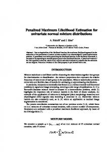
Examples and Comparisons sec:tion we illustr:a,te

processes as

...... , deviatl~s are

inn.owl.ticm proc:ess et

J(eJler,ated

sul)se,qm~nt

are set to 0

4

to nOI'ma.llty

recurs,ive equation

values are COJlll>'llted

CLU'-'V
- - - --

_

ooc-

. True'

~MLE C\I

0

j C\I I

~

..-;;;.........

'V I

0.02

0.04

0.08

0.16

0.0

0.32

0.1

0.3

0.2

Effective Bandwidth

Frequency

(c)

(d)

MA(4)

:

0.4

0.5

E 1',"

.'

. . ,#

/'

"

_ -17- -,'-// ,/

t/'

,t'

,selPA lEj·:.~.:·: : : : .:. .·.·.-,..: ·: ...J

C\I I

I'

True

__

. If':" .

""~.,,,

~LP

.

..,. 0.0

0.1

0.2

0.3

Frequency

Figure 2 (b)

(a)

0 T""

~

-

E

cx:>

2

~

c%

.s