Perceiving Motion While Moving

Journal of Experimental Psychology: Human Perception and Performance 2002, Vol. 28, No. 3, 731–747

Copyright 2002 by the American Psychological Association, Inc. 0096-1523/02/$5.00 DOI: 10.1037//0096-1523.28.3.731

Perceiving Motion While Moving: How Pairwise Nominal Invariants Make Optical Flow Cohere James E. Cutting and Wilson O. Readinger Cornell University Computer-generated sequences simulated observer movement toward 10 randomly placed poles, 1 moving and 9 stationary. When observers judged their direction of movement, or heading, they used 3 related invariants: The (a) convergence and (b) decelerating divergence of any 2 poles specified that heading was to the outside of the nearer pole, and the (c) crossover of 2 poles specified that heading was to the outside of the farther pole. With all poles stationary, the field of 45 pairwise movements yielded a coherent specification of heading. With 1 pole moving with respect to the others, however, the field could yield an incoherent heading solution. Such incoherence was readily detectable; similar pole motion leading to coherent flow, however, was less readily detectable.

Experiment 2. It too has received some experimental attention. The third purpose, which is unique to this pair of studies, was to account for the results of both from the same theoretical stance. That stance is considered subsequently, starting first with a description of optical flow in a stationary surround and then adding a moving object.

The movement of an observer through an environment of stationary objects creates a complex flux around him or her, called optical flow. Accurately registering this flux and acting on it underlies the everyday commerce and safety of all animals. This is particularly true for human beings. Technological means of conveyance have increased both speeds and risks. The tasks of finding our way through environments are several. Among these are (a) choosing a goal, (b) plotting a relatively direct route toward it, (c) avoiding stationary and moving objects along and near the path to it, and if it is a novel environment, (d) remembering landmarks sufficiently for a return. In this article, we focus on aspects of the second and third of these tasks— how pedestrians can be assured of being on a path to their goal while being alert to moving objects near their path. Following Gibson (1954), and going somewhat beyond him, we reserve the term movement for the position change of stationary objects relative to a translating observer. We use the term motion for the position change of independently translating objects, whether the observer is stationary or not. And finally, we use the terms displacements and flux when discussing both movement and motion at the same time, without distinguishing them. With this in mind, then, there were three purposes to the two experiments reported here. The first was to assess the effect of object motion on heading judgments during observer movement. This was the focus of Experiment 1, and it has received some attention in the experimental literature. The second purpose was to assess the detectability of object motion within movement, and this was done in

Piecemeal Characterization of Parallax in Optical Flow Three Types of Observer-Relative Movement and Four Classes of Object Pairs The array of flux around one as he or she moves is rich and can be parsed in many ways (e.g., Cutting, 1986; Gibson, 1966; Koenderink & van Doorn, 1975; Longuet-Higgins & Prazdny, 1980; Regan & Beverley, 1982; for reviews, see Lappe, Bremmer, & van den Berg, 1999; Warren, 1998). Recently, for purposes of heading determination in terrestrial travel, it has been useful to consider the relative horizontal displacements of pairs of objects, ignoring all other component vectors (Cutting, Alliprandini, & Wang, 2000; Cutting & Wang, 2000; Wang & Cutting, 1999b). Indeed, in a free-gaze heading detection task, Cutting et al. (2000) found that most fixations were at or near the horizon. Several classes of pairwise parallactic movements occur in the forward visual field: Objects converge or diverge. If the latter, the movements can be divided again: Some pairs decelerate apart, and some accelerate apart. All convergence in the forward field is acceleratory; all that in the rear field slows down. These three classes of pairwise relative movements and their consequences, are shown in Figure 1. Figure 1A shows the three types of movements for all other objects with respect to a given reference object and in front of a translating observer. In this case, the observer’s path is 20° to the left of the reference object. To hone in on his or her heading, a moving observer needs to register only two things—the relative horizontal movement and the ordinal depth of two objects (i.e., which object is nearer and which is farther away)—and then do this sequentially for several pairs of objects. With ordinal depth and relative movement known, several strong statements may be made concerning heading direction.

James E. Cutting and Wilson O. Readinger, Department of Psychology, Cornell University. Preliminary findings of the research reported herein were previously presented at a poster session during the annual meeting of the Association for Research in Vision and Ophthalmology, Fort Lauderdale, Florida (May 2002; see Readinger & Cutting, 2000). We thank Lois Lok-see Yue for help in testing the observers in Experiment 2, Frances Wang for discussion, and John Wann and an anonymous reviewer for comments on a draft. Correspondence concerning this article should be addressed to James E. Cutting, Department of Psychology, Uris Hall, Cornell University, Ithaca, New York 14853–7601. E-mail: [email protected] 731

732

CUTTING AND READINGER

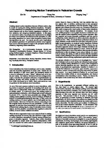
Figure 1. A: Layout around a moving observer and the observer-relative motions around a particular object 20° off his or her path to the right. All other objects in the forward field of view undergo one of three possible motions with respect to this object: They converge (white), they diverge and decelerate (black), or they diverge and accelerate (gray). B: Invariant relations among pairs of trees that specify heading direction. Diagonal lines represent lines of sight to two possible objects, one nearer and one farther. If a pair has crossed over in the field of view (left), and if observers can remember which objects were involved, heading is always to the outside of the farther object of the pair. If a pair converges in the field of view (middle) or decelerates apart (right), heading is always to the outside of the nearer member of the pair. C: A pair that decelerates apart. Heading direction is probabilistic, but most often to the outside of the farther member of the pair. The sequential relations sometimes found among these four relative motions are suggested in A. When the pedestrian is at Position 1, the reference object and the second object accelerate apart; at Position 2, they decelerate apart; at Position 3, they converge; and at Position 4, they will have crossed over.

First, a converging object pair specifies an invariant relation for the pair and the moving observer: The observer’s heading is always to the outside of the nearer member of the pair. This is true regardless of observer velocity or where in the field of view the pair might appear. There are no exceptions.1

Second, for pairs that decelerate apart, the same is true. One’s heading is always to the outside of the near member of the pair. But there is one caveat. Both objects must be within 45° of the heading direction. This constraint is not too limiting, considering that the data of Wagner, Baird, and Barbaresi (1981; see also Cutting, Wang, Flu¨ ckiger, & Baumberger, 1999) show that pedestrians look within this limit about 90% of the time. We call these two sources of information— convergent pairs and diverging decelerating pairs—pairwise nominal invariants about heading. That is, they name the side—left or right— of a given object, to which a moving observer’s heading must lie. Third (and different from the first two), pairs that accelerate apart offer no firm statement about heading without other information. There is no invariant relation. One can probabilistically state that heading is most often to the outside of the farther member of the pair— 69% of the time as calculated by Wang and Cutting (1999b). Thus, accelerating divergence is a heading heuristic and a reasonably good bet (Gilden & Proffitt, 1989). It is not an invariant, which necessitates complete specification of the state of affairs— or 100% probability. These three relations are shown schematically in Figures 1B and 1C, with lines of sight to near and far moving objects. The observer need not fixate anywhere in particular for these rules to hold. They are independent of gaze and thus a property of optical flow. Nonetheless, in a study of eye movements and fixations during simulated translation, Cutting et al. (2000) found that moving observers seek out and look at members of particular pairs—those that converge and decelerate apart. It would appear that these relative movements are (a) most informative to the pedestrian (as suggested in Figure 1) and (b) best detected on and near the fovea, where motion detection is best (Leibowitz, Johnson, & Isabelle, 1972). These relative movements are thus converted to retinal flow and have two important consequences. First, eye movements during pursuit fixation on one object subtract out its movement from optical flow, leaving it stationary in retinal flow. Second (and almost surely more important), this subtraction transforms the relative movements of all other objects to the fixation object into absolute retinal flux. In this manner, the nonfixated member of a converging pair will always move toward the fovea. In a similar manner, the nonfixated member of a decelerating and diverging pair will move increasingly more slowly away from the fovea. Finally, that in an accelerating diverging pair will sweep more rapidly away. These transformations, as accomplished by the pursuit eye movement system, should make at least some of the relative movements easier to register. Indeed, Cutting and Wang (2000) obtained results strongly suggesting that convergence of two objects is easy to see and use. However, they also found that decelerating divergence of two objects is considerably less salient and is likely to be detected best when the two are almost stationary with respect to one another (have little or no relative movement). Finally, they found that accelerating divergence of two objects seems basically to be a default category and that it psychologically corresponds to essentially all divergent displacement. 1

To the outside of the near member means within a 180° fan of that object for all convergences as measured from the near member and within a 90° fan for all accelerating convergences measured from the same point.

PERCEIVING MOTION WITHIN MOVEMENT

In addition (and new to the analysis presented in Figure 1), there are pairs that have crossed over in the field of view. If one can remember that two objects have converged and crossed over, heading will always be to the outside of the farther member of the pair. This too yields an invariant relation among objects, the moving observer, and his or her heading. It follows from the fact that converging items will, if the observer continues long enough on a straight path, always meet in the field of view; the nearer one will occlude the farther, and then the two will accelerate apart. Thus, what separates them from the latter category is only that one must remember having seen the crossover. This caveat is necessary: Whereas all crossover pairs accelerate apart, it is not the case that all pairs accelerating apart have crossed over. For example, any change of observer direction will change the orientation of the patterns as seen in Figure 1A and create a plethora of new pairs accelerating apart that never crossed over from the point of view of the observer. One can determine a natural history to these four sets of movements, at least for certain well-placed object pairs. Given a particular pair in a forward field of view, with the nearer one closer to the observer’s path, its set of movements may transform. If so, they will change in a particular order. In Figure 1A, consider again the reference object and, this time, also the second object slightly farther away and to the right. At the moment depicted, when the pedestrian is in Position 1, these two objects accelerate apart. By the time the observer has moved to Position 2, however, the pair decelerates apart. Moreover, by Position 3, the pair will converge, and by Position 4, they will have crossed over and again accelerate apart. Thus, this particular pair of objects would pass in stages through all four pairwise observer-relative movements shown in Figures 1B and 1C. The scheme outlined, and now elaborated, in Figure 1 has a more general alternative offered in the literature.

Parallax Field or Pairwise Constraints? Recently, Li and Warren (2000) found sets of results much like those of Cutting, Vishton, Flu¨ ckiger, Baumberger, and Gerndt (1997) and Cutting et al. (1999). That is, they found that feedback from eye movements was generally necessary for heading determination in a simulation in which observers passed through a dot field, but that such feedback was generally unnecessary when passing through an environment with information about how stationary objects are laid out in depth. Moreover, they attributed their results to the global parallax field of displacements in an account quite similar to that of Cutting et al. (1997, 1999) and Wang and Cutting (1999a, 1999b). The differences between Li and Warren’s (2000) approach and ours are less than they might first appear. Li and Warren focused on the whole field of parallax movements; we focus on a selected few that compose the larger field. We believe that not all of the field is equally informative and that observers seek out and use the invariant information there. Nonetheless, there is, in principle, no difference between these approaches. Indeed, an additional purpose of this study is to further increase the number of objects in the field of view of our observers, approaching a dense field, to demonstrate the statistical and conceptual continuity between them. Dense fields of objects in parallax have more invariants, and we continue to search for evidence that observers use these. Moreover, Li and Warren also focused on the importance of a few

733

reference objects in the parallactic field, and this is a theoretical nod in our direction. Movements around such objects are well captured by our piecemeal approach.

Moving Observers, Mobile Objects, and Heading Judgments There are a number of previous studies investigating the effect of object motion on heading judgments. Warren and Saunders (1995) and Royden and Hildreth (1996) both conducted experiments with simulated moving observers and object motion within a few degrees of their heading. Both used mobile objects and stationary surrounds consisting of fields of dots, with no overt segregation of the two prior to stimulus onset. And both sets of studies found that the motion of an object affected perceived heading direction, particularly when true heading was occluded. Certain details of their results conflicted, and discussion of this is deferred until our discussion of the first experiment, in which we provide a resolution. Cutting, Vishton, and Braren (1995) also conducted a set of studies with mobile objects and moving observers. However, their studies had a well-identified object (a simulated human walker strolling through the scene) and a differentiable stationary surround (a sparse forest of a dozen or more trees). They found no apparent effects of the presence of a mobile object on perceived heading direction when simulated fixation was on a stationary object, but they found generally striking interference in heading judgments when simulated fixation was on the mobile object.2 We assume that the results for all three studies—a general decline in heading performance in the presence of a scrutinized object in motion— have a similar cause. That is, the pairwise relations among the mobile object and the many stationary objects during observer translation are out of kilter with the optic flow of an observer through a stationary environment. These changes in information created systematic biases in perceived heading. Warren and Saunders (1995) modeled this bias by averaging all flow vectors: those of the mobile object and the moving surround. Whereas their model accounted nicely for their own results, it could not account for those of Royden and Hildreth (1996). Here, we take a different tack. We consider all pairwise relative movements and provide the general framework for an account of both studies, and we set the context for discussion of detecting moving objects, the topic of Experiment 2.

Experiment 1: Heading Judgments With and Without a Moving Object Method Stimuli. Stimulus sequences were generated on a Silicon Graphics Indy (Model R5000) at 34 frames/s. Viewers sat about 0.5 m from the screen, yielding a 30° wide display seen at a resolution of about 40 pixels/degree. Each sequence was 4 s in duration. It consisted of simulated observer

2

An exception to this latter effect occurred when the moving object traveled a path directly toward the observer—much like oncoming traffic along a sidewalk or roadway. Here, there was no interference; indeed, performance was even somewhat better than when all environmental objects were stationary.

734


translation (a dolly) at 1.23 eye heights/s (about 2 m/s for a pedestrian 1.75-m tall with eyes 1.6 m off the ground). Translation was generally toward a collection of 10 poles, with a small additional rotation (a pan) to keep the center of that collection in the center of the display. A schematic plan view rendering the layout is shown in Figure 2A, with an observer taking a path 3° to the left of the middle region of the poles. Poles were planted stochastically within 10 rectangular areas. Each area was 2.56 eye heights in depth, but the areas varied in width. Pairs of regions straddled the depth axis measured from the initial position of the observer. From farthest to nearest the observer, the five pairs of regions were 1.55, 1.30, 1.05, 0.80, and 0.55 eye heights in width, respectively. This arrangement forced a clustering of poles and simulated a locally dense region of objects as seen by the viewer. For various analyses, the poles were numbered from left to right according to their positions at the end of a trial, as shown in Figure 2C. Mean initial and final horizontal separations of Poles 0 and 9 were 5.8° and 9.2°, respectively. All poles remained visible during the course of every trial. All poles were 1.69 eye heights tall. Relative distance from the observer was indicated by three sources of information: (a) relative pole height, (b) relative pole width, and (c) height in the visual field (angular elevation) of the base of the poles. Intrinsic pole size was specified by the horizon, which intersected each pole at 59% of its height. The sky was light blue, the ground plane was brown, and the poles were dark gray. The horizon was true, not truncated at a given depth. The initial and final frames from a sample trial are shown in Figures 2D and 2C, respectively. On half the trials, 1 of the 10 poles translated linearly to a slight extent over a featureless ground plane.3 The other poles were stationary while the trial simulated observer movement toward all 10. The motion of the mobile pole was sideways (orthogonal to the depth axis in Figure 2A), at a constant environmental velocity of 0.031 eye heights/s. This motion is only about 5 cm/s for a 1.8-m pedestrian with an eye height of 1.6 m. The projection of this motion was added to (or subtracted from) the observer-relative movement of the pole were it stationary. Total environmental displacements during the trials, left or right, were 0.125 eye heights. Angular velocities varied with simulated distance of the pole from the observer. Mean image speed (horizontal absolute velocity) for stationary poles was 0.31 degrees/s (SD ⫽ 0.24 degrees/s; range ⫽ 0 –1.1 degrees/s). Mean image speeds for the poles in motion were 0.41 degrees/s (SD ⫽ 0.33 degrees/s). All means were a bit more than an order of magnitude above the foveal threshold for motion detection (about 0.025 degrees/s; Leibowitz et al., 1972). On a given trial, the mobile pole had the greatest image speed of all poles in 21% of all trials (chance ⫽ 10%). It had the least speed in 15% of all trials. Viewers were presented random sequences of 160 trials. Half of these had a mobile pole: 10 pole positions ⫻ 2 directions for the mobile pole (left and right) ⫻ 2 sides of approach (observer approaching the pole cluster with the majority of poles to the left or to the right) ⫻ 2 initial gaze– heading angles (1° and 3° from the center of the pole cluster). Final gaze– heading angles were 1.4° and 4.2°. Maximum simulated rotation rate was about 0.3 degrees/s. This rate is well below the 1 degrees/s at which eye muscle feedback might be needed for heading judgments (Royden et al., 1992). In addition and randomly intermixed, there were 80 other trials yoked to these, with identical initial pole positions but with no mobile pole. Prior to the test sequence, observers responded with feedback to a few practice trials with gaze– heading angles of 5° and 9°. No feedback was given during the course of the experiment. Observers and task. There were 15 members of the Cornell University community who participated in the task. All were naive to the purposes of the experiment at the time of their participation. Most volunteered for course credit; 4 were paid. Each participated singly and had normal or corrected-to-normal vision. Each was told to look wherever they liked during the course of the trial, but to try to locate the direction they were headed. At the end of the trial, a mouse-controlled red probe bar appeared on screen. It was located beyond the poles, near the horizon and at a distance of 39 eye heights. It was 2 eye heights tall, and could slide along

Figure 2. An example trial and its structure. A: A plan, scaled view of its layout, the locations of the observer, and the regions within which poles could have been randomly placed. D and C: Beginning and ending frames, respectively, of the 4-s sequence simulating observer movement along a path 3° to the left of the poles, and with a pan to the right to keep the center of the region of poles in view. The moving pole on this particular trial was Pole 8. Pole numbers and positions correspond in A, B, and C. B: 19 pairs of poles involved in heading invariants: 14 converging and 5 decelerating apart. Each arrow points in the specified heading direction; its stem connects the two poles involved in a particular invariant relation, and the base of the arrowhead delimits the edge of the response region allowed by the particular invariant pair. Eighteen of these invariants specify that heading is to the left; one pair involving Pole 8 yields a heading result incoherent with the rest, specifying that heading is to the right.

3 Longuet-Higgins and Prazdny (1980) considered the case of objects moving freely in a textured environment. In such cases, the occlusion and disocclusion of texture at leading and trailing edges of the base of the object serve as solid information about object movement. In our study, we did not display such information, because we were interested in relative motions, not occlusions and disocclusions.

PERCEIVING MOTION WITHIN MOVEMENT the ground plane. The viewers’ task was then to move the probe to the location they thought corresponded to their heading, and press the left mouse key. As they moved the mouse, the poles occluded the probe. If observers wished, they could repeat the trial by pressing the middle mouse key. The task took about 15–30 min to complete, depending on the number of repeated trials. Eye movements, simulated pursuit fixation, and their dissociation. Some concerns about our approach focus on methodology and the particular relations among the stimuli, the observers’ choice of fixation, and their eye movements. These concerns divide two ways. First, our displays simulate translation with pursuit fixation during the translation slightly off to the side. That is, the display combines the camera motions of a dolly and a very slight, horizontal pan (generally, less than 1 degree/s, and here, always less than 0.3 degrees/s). This general technique is common in the literature and had been used by Regan and Beverley (1982), Cutting (1986), Warren and Hannon (1988), and Royden, Banks, and Crowell (1992). With the observer’s gaze fixed at the center of the screen, this methodology dissociates retinal stimulation and feedback from eye muscles. Thus, if the simulated eye rotation is initially 1 degree/s to the right, real eye rotation is 0 degrees/s. The dissociation, then, is 1 degree/s. Fortunately, feedback is unnecessary at such modest rotation rates (Royden et al., 1992) and perhaps at even greater rates (Cutting et al., 1997, 1999; Li & Warren, 2000). Second, we allow the observer to scan the simulated pursuit–fixation display however he or she wishes (Cutting et al., 2000; Cutting & Wang, 2000). If the observer fixates anywhere other than at midscreen, sampling information over its surface during the trial sequence, the dissociation continues and its magnitude remains constant. In the example above, it would remain 1 degree/s. Thus, whether simulated and real rotations are 3.5 degrees/s and 2.5 degrees/s (to the right) or ⫺2.5 degrees/s and ⫺1.5 degree/s (to the left), the magnitude of the dissociation remains invariant. This has been important in computational models of heading, such as those of Longuet-Higgins and Prazdny (1980) and Rieger and Lawton (1985). The dissociation may appear unnatural—and it is certainly different from driving a car— but it is not unnatural. In sailing, one’s heading (the direction the boat is pointed) is almost always different than one’s course (the direction one is going). Skippers typically align part of the boat with a stationary distant object to hold course temporarily, but because heading and course are dissociated, this tactic causes the angle between them to change slowly, just as in our studies. Skippers also continually look around them, gathering information about their course and safety.

735

these analyses, however, were there any differences in side of approach of the observer to the pole cluster, Fs(1, 14) ⬍ 1, so we collapsed across them in further investigations. Nominal responses. In general, observers were quite accurate in their heading judgments on trials in which all poles were stationary. Mean nominal performance was 79% correct. There was a reliable effect of heading angle, F(1, 14) ⫽ 73, p ⬍ .01: Observers were 68% correct for trials with initial heading angles of 1° and 90% correct with initial angles of 3°, as shown in Figure 3A. More interesting, however, is that these performance levels are considerably higher than in previous studies. When pooling the results of Cutting and Wang (2000) and Cutting et al. (1999), for example, we found observer performance at trials with mean initial heading angles of 1° and 3° was only 60% and 72%, respectively. We attribute the superior performance here to the considerably increased number of invariant constraints imposed by 10 objects as opposed to 2 (Cutting & Wang, 2000) or even 7 (Cutting et al., 1999). Nominal performance on nonrigid trials was slightly but not significantly lower, F(1, 14) ⬍ 1: 58% and 86% on trials with gaze– heading angles of 1° and 3°, respectively, also shown in

Nominal Results, Absolute Results, and Preliminary Discussion We have found it useful to analyze heading responses three ways—nominally, absolutely, and categorically. Nominal responses are those that consider whether the viewer responded by positioning the probe to the correct side of the center of the screen (Cutting, 1986; Cutting et al., 1999). As noted earlier, the simulated fixation is at midscreen, and modest rotation of the environment occurs around it. Absolute responses are those measuring how far to the left or right of midscreen the probe was placed (Cutting et al., 1999). These measure the perceived relation of the line of gaze to the heading vector, which can be compared with the actual gaze– heading angle. Discussion of the absolute responses leads to an important interaction and a comparison with the literature. Finally, categorical responses are those measured within particular bounds dictated by pole locations and invariants (Cutting et al., 2000; Cutting & Wang, 2000; Wang & Cutting, 1999b). Discussion of the categorical responses leads to the idea of permissible response regions and an analysis of multiple invariants. These are deferred until discussion of Experiment 2. In none of

Figure 3. Main results for Experiment 1. A: Nominal performance for rigid and nonrigid trials at the two initial gaze– heading angles. B: Absolute response eccentricities for the same trials. Error bars indicate one standard error of the mean.

736


Figure 3A. There was no reliable interaction of rigidity and heading angle, F(1, 14) ⫽ 2.0, p ⬎ .15. Absolute responses. Mean absolute heading error for rigid arrays was 40 min of arc (0.66°), also considerably superior to previous studies (Cutting & Wang, 2000; Cutting et al., 1999). Nevertheless, it seems likely that this improvement was partly due to the exclusive use here of relatively small heading angles. Again, there was a strong effect of heading angle, F(1, 14) ⫽ 35.7, p ⬍ .01, typical in this type of research. Mean eccentricity of heading placements was 1.29° for the trials with an initial heading angle of 1° (final angle of 1.4°) and was 3.00° for trials with an initial angle of 3° (final angle of 4.2°). On trials with a mobile pole, absolute judgments were a bit more varied, but not statistically, F(1, 14) ⬍ 1, with a mean absolute error of 49 min of arc (0.82°). Heading placements were also not reliably different from those of rigid trials, F(1, 14) ⬍ 1: 0.85° and 3.31° for angles of 1° and 3°, respectively. In addition, there was no reliable interaction, F(1, 14) ⫽3.5, p ⬎ .08. These results are shown in Figure 3B. Interaction of motion direction and depth. Despite the overall similarity of results for rigid and nonrigid trials, there was systematic variation in heading placements for nonrigid trials, depending on which pole was in motion. Figure 4A aids in explaining this trend. In each of the five schematic plan views of the pole regions, the mobile pole is depicted as if residing in one of two paired cells receding in depth. It is also depicted as if always translating to the right. If such translation occurred for one of the nearest poles, it might contribute to the impression of increased counterclockwise rotation (in plan view) of the complete array of poles. Plan-view counterclockwise rotation corresponds to the projected retinal flow when one looks off to the right of one’s path (see also Kim, Turvey, & Growney, 1996). That is, all objects rotate around the fixated location, simulated here among poles farther back. Thus, the fruits of increased counterclockwise rotation on such trials might be that one’s judged heading is farther left than it would be from an identical stationary array. The opposite would occur when one of the farthest poles translates rightward. That is, such motion might contribute to the impression corresponding to a plan view of an array with more clockwise rotation. Plan-view clockwise rotation is the same as the retinal flow during pursuit fixation off to the left of one’s path. Thus, one’s judged heading might be farther right when distant poles translate to the right. With respect to these near and far anchors, poles residing in intermediate locations should yield intermediate results. And this interaction is exactly what we found, as shown in Figure 4B. Strongly consistent with this conceptualization of perceived heading differences was a linear trend across differences in yoked stimuli, which occurred on nonrigid trials when the mobile pole created a coherent array of invariants, F (1, 14) ⫽ 406, p ⬍ .01. The account just given is very much in tune with that of Perrone and Stone (1994, 1998), whose model pools different displacements at different depths. Our account is actually different but yields the same result. We discuss our account here in detail, because it is the same account that we use in considering the results of Experiment 2. Thus, instead of pooling flux at different depths, we consider simply the probability of a mobile pole generating new invariants compared with its stationary counterpart in its yoked comparison trial. A near pole translating to the right is likely to be coupled with a pole more distant from the observer.

Figure 4. A: Icons of the layout of poles in Experiment 1 and highlighted regions in which mobile poles resided, dividing the trials into five categories. The scaled length of the arrows corresponds to their projected motion; in simulated space, they were identical but at different depths. B: Results for differences in judged heading between stationary arrays and those with one pole in motion, plotted as a function of the relative depth of the mobile pole in the array and as if mobile pole motion were always to the left. Error bars indicate plus or minus one standard error of the mean. Also shown is the change in the inner boundary of the permissible response region as a function of the mobile pole. The parallel between the two functions lends support to our account that changes in heading are due to changes in boundaries of the response regions.

Whether the far pole crosses, converges with, or decelerates away from its nearer mate, the pair specifies a heading to the left. In a similar manner, a far pole translating to the right is more likely to be the more distant member of an invariant pair and to specify heading to the right. There is, therefore, a simple statistical prediction that mobile poles at different depths will result in opposite heading biases. We tested this idea by assessing differences in what we call the inner permissible boundary of the heading responses across all trials for each viewer. This boundary is marked by the location of the pole closest to the center of the screen, which dictates that all responses must be to its outside. Gaps to its outside that are away from the center of the screen generally lie within the permissible response region. The locations of this inner boundary were differ-


737

ent for trials with a mobile pole compared with their matched-pair stationary controls.4 These results are also shown in Figure 4B, plotted again as if pole motion were always to the right. Results show that the mean boundary shifts mirror the shifts in responses. We believe the former are the likely cause for the latter: When nearest poles were in motion, these boundaries shifted in the same direction and to about the same degree as responses, and when farthest poles were in motion, the boundaries shifted similarly. The parallel between the change in boundary and the change in responses lends credence to our account, which accrues in the analysis of previous results in the literature.

Comparison with the Literature and Resolution of Conflict Both Warren and Saunders (1995) and Royden and Hildreth (1996) investigated the perception of heading during simultaneous movement and motion. Both used dot-field stimuli without other depth information and stimuli simulating translation without rotation (a dolly without a pan). In both, the observer’s approach was roughly orthogonal to a wall of dots, and in the case of Royden and Hildreth, to two transparent walls. Mobile objects consisted of squares, also oriented orthogonally to the observer’s path. These mobile objects translated obliquely with respect to the observer in front of the planar background(s). Sometimes these squares were transparent, sometimes they were not; when they were not, they sometimes occluded the heading direction, or aim point, of the observer. Both sets of studies found that observers could locate their headings reasonably accurately, particularly when the mobile object did not occlude the aim point. Nonetheless, response biases occurred in each that were directly related to the direction of object motion. Most interesting, the results of Warren and Saunders (1995) and Royden and Hildreth (1996) were in opposite directions. In the former studies, the perceived heading was shifted in the direction opposite to the projected motion of the mobile object, whereas in the latter, the shift was in the same direction as the mobile object. Both sets of authors worked hard at reconciling differences, but no definitive account for both effects was found. Here, we present a new scheme to account for their differences, one that is also consistent with our theoretical stance. Figure 5A shows two schematic plan views, one of the layout of stimuli used by Warren and Saunders and the other of the stimuli used by Royden and Hildreth. In each case, the mobile objects are shown translating to the right, in the manner they would have in their respective studies. For didactic purposes, consider a vectorial decomposition of the object motion in the two cases. Both mobile objects had one component vector orthogonal to the observer’s approach to the wall (or walls) of stationary dots. Its direction was the major experimental variable in both sets of studies. Again, in Figure 5, this component is rightward, although it occurred equally often to the left in the studies. However, the moving object used by Warren and Saunders (1995) also moved toward the observer; that of Royden and Hildreth (1996) moved with the observer and at the same velocity, toward the dot walls. The projections of these motions at the observer’s eye are quite different. Heading biases opposite to object motion. As mentioned above, the stimuli of Warren and Saunders (1995) consisted of fields of dots. This is important because there was no information

Figure 5. An explanation to resolve the conflict between the results of Warren and Saunders (1995) and Royden and Hildreth (1996). Top: Plan views of the general stimulus situation in the two sets of studies. Middle: Motion of the object decomposed into two vectors. The moving object of Warren and Saunders translated toward the observer and away from the dot wall; that of Royden and Hildreth translated toward the dot walls at the same velocity as the observer. Bottom: The two conditions in Experiment 1 that these situations mimic.

about the relative depth of any pairs of dots. Thus, our system outlined in Figure 1B cannot generally apply. Nonetheless, a modification of it can apply. Wang and Cutting (1999a) showed that the presence of converging dots in a flow field of environmentally stationary dots eliminates the possibility that one’s heading can lie between them.5 One can see in Figure 1B, while ignoring depth, that this must be true. As suggested before, by 4 Only coherent trials were used in this analysis. Incoherence is assessed as follows: The heading constraints specified by all invariant pairs are first registered, then compared. If the leftmost boundary of the permissible response region for one pair occupies the same location or is to the right of the rightmost boundary of any other pair, then the trial is incoherent. If there were no left or right boundary on a given trial, the edge of the screen was used. All other trials are coherent, regardless of whether there is a mobile pole. 5 Convergence is measured along the horizontal meridian. If one considers any two dots that converge on any vertical slice through the flow field, then one’s instantaneous heading cannot lie between vertical lines passing through those two dots (Wang & Cutting, 1999a).

738


itself this depth-blind information is sufficiently robust for a heading algorithm based on it to perform as well as any in the literature. Applied to the Warren and Saunders (1995) stimuli, the dots of the moving object will generally move faster across the screen than those of the dot wall behind and near it. This means that object dots are likely to converge with wall dots, particularly those near the leading edge of the object. If members of both sets of dots are provisionally considered part of the same array, then the perceived heading should be displaced toward the trailing edge of the moving object— or, more pertinently, in the direction opposite to its movement. In Figure 5, this would be to the left. And this is exactly what Warren and Saunders found. This is most similar to the situation in the leftmost panel of Figure 4A, which is also shown in Figure 5. Heading biases in the same direction as object motion. Applied to Royden and Hildreth (1996), a different picture emerges. Although consisting of dots, their stimuli had some different attributes. The mobile object moved with the observer at the same velocity toward the dot walls and had a lateral component of motion. The dots composing the object did not expand, nor did they contract. Lack of expansion or contraction is optical information during observer translation for an object at functionally infinite depth.6 This object may not have been perceived as such in all situations explored by Royden and Hildreth, but there is at least the situation in all of their contexts of information conflict. Such conflicts typically yield compromising percepts (Cutting & Vishton, 1995), such as an object at intermediate, but not infinite, depth. If the mobile object contained information about infinite depth or simply depth beyond the first dot wall, then its rightward motion (as in Figure 5) would contribute to the perception of a plan-view clockwise rotation of the array. Such a situation is shown in the rightmost panels of Figure 4A and also in Figure 5. This would push the perceived aim point to the right of where it might ordinarily be perceived and in the direction of the object motion (and opposite to that of Warren & Saunders, 1995). That is, the more distant dots of the mobile object would converge with nearer wall dots and provide information for heading beyond the leading edge of the object. With such a depth interpretation, this is what the Hildreth (1992) model would predict, and this is what Royden and Hildreth (1996) found. Thus, using the general scheme proposed here, we can account for the discrepancy in results between the two studies as well as for the interaction between distance and motion direction reported in Figure 4B.

Categorical Responses and Discussion Gaps and permissible response regions. When the relative movements are considered between two stationary objects, there are three possible response categories: one between them and one on either side. We will call these gaps. They are bounded by the poles, or in the case of end poles, they are bounded by the pole and the edge of the display screen. Cutting and Wang (2000) analyzed heading responses in this manner for simulated movement through environments with two objects (three gaps), Cutting et al. (2000) analyzed them for four objects (five gaps), and Wang and Cutting (1999b) analyzed them for environments with as many as seven objects (eight gaps). With 10 poles, there are 11 gaps, creating a wider variety of possibilities. The set of invariants on a given trial could constrain responses to the left of any pole, to the right of any pole, or between almost

any pair of poles (except Pole Pairs 0 –1 and 8 –9). This creates 50 possibilities. Of these, 41 occurred during the experiment. Thus, it seemed most prudent to condense the results, to look for systematic patterns across these possibilities and to consider whether the observers’ responses fell between the constraining poles. In principle, these constraining poles create permissible response regions with different numbers of gaps. Consider a one-gap permissible response region, for example, between Poles 6 and 7. To achieve such a situation, Pole 5 might converge with Pole 6 (the closer of the two), and Pole 8 might have just crossed in front of Pole 7. Consider next a permissible response region with nine gaps. Pole 0 might converge with its nearer neighbor, Pole 1, constraining responses to all gaps to the right of Pole 1. Because no trial in the experiment had fewer than two invariant pairs, however, the upper limit for a permissible response region was eight gaps, and this limit was created with three invariant pairs. If, for example, Poles 0, 1, and 2 all converged (creating Pairs 0 –1, 0 –2, and 1–2), and if Pole 3 were the closest and Pole 2 the next closest, there are eight permissible response gaps to the right of Pole 2. Indeed, the range of permissible response gaps in the experiment fell between one and eight. Their relative occurrences are shown in Figure 6A and are divided two ways: those arrays allowing a response region that included the external gaps (those between end poles and the edge of the screen) and those confining responses to the interior of the array. Next consider performance as a function of the number of gaps in the permissible response region. These gaps are plotted in Figure 6B, separately for stimuli in which the regions include end gaps and for stimuli in which the regions do not. Clearly there is no difference, F(1, 14) ⬍ 1. In both cases, performance increased from about 60% to perfect performance as the number of permissible gaps increased from two to eight. This increase makes sense in that as more gaps become permissible, the increasingly wider region of the screen allows for more correct responses. To test for this increase, we sorted individual results into bins (permissible gap sizes of 1 and 2, 3–5, and 6 – 8) and computed their percentage correct placement of the probe within those bins. Results confirmed what can be seen in Figure 6B; the main effect was reliable, F(1, 14) ⫽ 10.23, p ⬍ .01, with means of 67%, 77%, and 92% correct. Also plotted in Figure 6B are the mean widths of the permissible areas in degrees of visual angle. The great difference in the widths of permissible response regions for stimuli allowing external gaps and those allowing only internal gaps, coupled with the similarity in their performance, suggests that the end gap plays no particular role in responses. Heading accuracy and the number of invariant pairs. Finally, consider the number of invariant pairs in given stimuli. These varied from 2 to 22. At the bottom of Figure 7 is the distribution of invariant pair numbers across all stimuli. We next plotted performance (correctly placing the probe within a permissible gap) 6 The lack of expansion or contraction could surely be construed as an object traveling at the same speed, but it need not be. If some module of the visual system does not seek segregation of movements (Warren & Saunders, 1995) but simply tries to make coherence of the array with no object motion in it, the only solution is that the dots on the moving object are at infinite distance.


739

invariants per trial. There may have been, but it will not necessarily show in this analysis. Although there may be many invariant pairs in a given trial, it is likely that only one or a few will govern the particular boundaries of the permissible region for heading responses. Consider the sample trial in Figure 2, ignoring the Pole Pair 7– 8. Eighteen of the invariant pairs specify that heading is to the left, but only Pair 0 –1 specifies that it is to the left outside; Pairs 2– 4, 2–7, 2– 8, and 2–9, for example, all specify only that it is to the left side of Pole 2. Thus, if one registered those 17 coherent invariant pairs, but not Pair 0 –1, one might place a heading response in the gap between Poles 1 and 2. This would adequately follow the bulk of the specifications, but for the array as a whole, it would be incorrect.

Overview Results of this study of heading judgments replicate and extend previous work. On trials in which all poles were stationary, heading responses were largely governed by the boundaries of permissible response regions, which in turn were specified by pairwise invariants (Cutting et al., 2000; Wang & Cutting, 1999b). Heading responses on trials with mobile poles were similar, but were shifted in the direction opposite mobile pole motion when it was near (replicating the results of Warren & Saunders, 1995) and were shifted in its same direction when it was far (replicating the results of Royden & Hildreth, 1996). The likely cause for all of these shifts was the change in the permissible response boundaries. We also found that for the generally fixed density of objects used in these studies, the wider the permissible response region, the more accurate were the observers’ categorical responses, and performance did not increase with the number of invariant pairs in the stimulus. Together these results suggest that finding one or a few invariants does not suffice. Observers must continue to seek Figure 6. A: Relative frequency of arrays allowing external gaps (those between the outermost pole and the side of the screen) and of those allowing only internal gaps (between poles). B: Categorical heading performance (top) for stationary-array stimuli in Experiment 1 as a function of the number of gaps permitted by invariant constraints. Mean widths (bottom) of the region of permissible responses for both stimulus types. Because the screen width was 30°, the right ordinate is scaled to the left ordinate, showing that arrays allowing external gaps had permissible regions of a little more than half the screen, whereas those allowing only internal gaps occupied more than a quarter of the screen.

as a function of the number of invariant pairs in the array. The results at the top of Figure 7 show a remarkably flat function, with a mean performance of 79% and a standard deviation of only 5%. The data for the functions at 2 and 21 invariant pairs were eliminated, because there were fewer than five observations for each, but performance was 100% for both. Because there were wide variations across viewers in the number of times each of these 21 stimuli occurred, we again sorted the individual responses into bins—this time of those to stimuli with less than 5 invariants per array, between 5 and 10, and more than 10. Mean performance within these bins was 81%, 76%, and 82%, respectively, with no main effect, F(2, 28) ⫽ 1.3, p ⬎ .25. It may seem odd that there was no redundancy gain (Garner, 1974), or improvement in performance, with increasing number of

Figure 7. Top: Categorical heading performance for stationary-array stimuli in Experiment 1 as a function of the number of invariant pairs in the stimuli. Bottom: Relative frequencies of each type of trial.


740

out their heading. To do so, they must scan the array of objects in search of invariants that constrain the permissible region of heading responses, and these are often slow to emerge. In an eye movement study, this is exactly what Cutting et al. (2000) found: Observers consistently sought out invariant pairs as opposed to heuristic pairs (objects accelerating apart), and dwelled on them longer, before making a response.

Detecting Motion Within Movement The second focus of this article is the prospect of detecting an object’s motion within optic flow. In all cases, we assumed the object is moving along the same plane as the observer. How might an observer detect motion within movement? Gibson (1950) outlined a scheme in which object motion stood out against the uniformity of an unmoving background, and movements created a background of change everywhere. Frost, Wylie, and Wang (1990) found neurological evidence for such segregation. The combination of motions and movements, however, can often make them difficult to separate (Probst, Brandt, & Degner, 1986). Below, we consider three ways they might be segregated and then a fourth that we develop. All motions are considered in only their horizontal component, because this would be the hardest to detect. First, in many circumstances, local optical velocity could be used to predict the difference between motion and movement (Brenner, 1991; Jain, Militzer, & Nagel, 1977; Wertheim, 1995). The data of Wagner et al. (1981) suggest that pedestrians look at stationary objects about 60% of the time. If we are fixated on a stationary object near our path, any object in motion is likely to be the object with fastest or slowest motion in the local field of view. This idea has been used with some success in the computational literature (see Hildreth, 1992, for a review). The data of Wagner et al. also suggest that the other 40% of the time we look at objects in motion. If one fixates the object in motion, the patterns of movement of stationary objects around it can be complex, but such movements are critical for detections of collisions and bypasses. Cutting et al. (1995) noted that when a pedestrian is on a collision course with a moving object, the flow of stationary objects around it was uniform in direction and with a magnitude the reciprocal of distance. When the mobile object would pass behind, near and far stationary objects generally moved in opposite directions; when the mobile object would pass in front, all objects moved in a uniform direction with nearly uniform flow. Second, binocular disparities may help segregate motion from movement (Kellman & Kaiser, 1995). Indeed, motion and stereo information have been shown to interact (Turner, Braunstein, & Andersen, 1997), particularly at and near threshold values for each (Tittle, Perotti, & Norman, 1997). However, stereoscopic information may not be useful in situations in which object motion is slight—the situation investigated here— or when the object in motion is farther away than about 30 m (Cutting & Vishton, 1995). Third, familiarity with environmental objects will go some way toward specifying what is in motion and what is not. Indeed, Cutting et al. (1995) specifically used this information in their study of collisions and bypasses. Cars, people, and animals can translate to new positions; trees, buildings, and rocks normally cannot. But of course, at any given moment, cars and other objects can either be translating or be stationary. Thus, familiarity cannot be the sole means by which motion within movement is detected.

Fourth (and the focus of this experiment), the array of invariants might yield patterns that would isolate a moving object. Here, we removed binocular disparities, familiarity, and, as much as possible, differences in image motion as variables that could aid in the detection of motion during movement. Again, we presented viewers an array of identical poles, one of which (albeit perhaps somewhat mysteriously) was mobile to a very modest degree. Our view is that the three invariants listed above should go a good way toward predicting whether such motions are detectable. That is, in a manner similar to Longuet-Higgins and Prazdny (1980), we can assess any assumption of stationarity of objects in an environment (a variant of the rigidity assumption) by measuring potential violations. In a dense field, an object in motion is likely to create pairwise relations with stationary objects that yield a heading direction (were all objects assumed to be stationary) that is inconsistent with the heading direction specified by pairs of stationary objects. Indeed, this is what we tested in our second study.

Experiment 2: Judgments of Object Motion While Moving Method Stimuli and task. Trials were patterned after those in Experiment 1, except that here, all trials had a mobile pole. In Experiment 1, the mobile pole always had a uniform amount of environmental motion—a mean velocity of 0.031 eye heights/s. Here, mean velocities for this pole were 0.031 eye heights/s (as before) and also less— 0.023 and 0.016. These correspond to 5, 3.75, and 2.5 cm/s. Corresponding mean image speeds for the mobile pole were 0.41, 0.37, and 0.33 degrees/s (SDs ⫽ 0.33, 0.30, and 0.25 degrees/s, respectively). We call these conditions those with most, middle, and least motion, respectively. Again, all means were a little more than an order of magnitude above the foveal threshold for motion detection (about 0.025 degrees/s; Leibowitz et al., 1972). On a given trial, the mobile pole had the greatest image speed of all poles in 21%, 16%, and 14% of all trials for conditions of most, middle, and least motion, respectively (chance ⫽ 10%). The mobile pole had the least speed in 15%, 13%, and 12% of all trials, respectively. At the end of each trial sequence, the last frame remained on the screen and the mouse-controlled cursor appeared. Observers were instructed to move the mouse freely left and right on the mouse pad. The horizontal extent of the screen (1,280 pixels) had been divided into deciles, left to right. Placement of the cursor within a decile changed the color of a pole from dark gray to bright red, highlighting it. By counting poles ordinally left to right, we assigned each a screen decile for such cursor placement. With this interface, observers could select the pole they thought was in motion during the trial. If they were satisfied that the pole of their choice was red, they clicked the left mouse button and the next trial began, with a 1-s announcement of its trial number. If observers were unsure of the translating pole, they could click the center mouse button and see the trial again. They were allowed to repeat any trial as often as they liked. Two types of responses were recorded—the pole chosen by the observer and, for selected analyses, the number of times the observer viewed each trial. Responses were recorded in computer files. Each observer participated individually, watching three randomly ordered sequences of 80 trials. These were factorial combinations of a mobile pole in the 10 different pole positions (planted randomly in regions as shown in Figure 2A) ⫻ 2 directions of motion (environmentally left or right) ⫻ 2 observer heading directions (to the left or to the right of the pole system’s center) ⫻ 2 initial gaze– heading angles (1° and 3°). Order of the three conditions was fixed in a downward staircase: Observers first watched the sequences with greatest motion of the mobile pole, then the

PERCEIVING MOTION WITHIN MOVEMENT middling, followed by the least (0.031, 0.023, and 0.016 eye heights/s, respectively). Observers. There were 15 different members of the Cornell University community who participated and were paid for their participation. Again, all were naive to the purposes of the study at the time of testing, had normal or corrected-to-normal vision, and were tested singly. Observers were told to try to find the pole that moved independently on each trial, looking anywhere they liked. Each observer received a few practice trials with feedback before beginning the first sequence. This familiarized each with the task and the interface. On such trials, the mobile pole moved 6 eye heights and, consequently, was extremely easy to detect. No feedback was given during the course of the experiment. With practice and debriefing, the experimental session lasted between 45 and 90 min, depending on the number of trials repeated. Multiple pairwise analyses for a sample trial. The most complex analyses in these studies concerned the stimuli, not the responses. Consider the trial shown in Figure 2. Again, its initial and final frames are shown in Figures 2D and 2C, respectively, along with a plan view of the layout of these poles in Figure 2A. Given 10 poles (n), there are 45 pairs of poles to consider, n ⫻ (n ⫺ 1)/2. On this sample trial, Pole 8 was in motion, the penultimate on the right. During the trial, it translated leftward by 0.125 eye heights as the observer moved forward 4.94 eye heights and to the left of the stationary poles by 3°. When comparing Figures 2C and 2D, notice that with the observer’s movement, this pole was actually displaced to the right. That is, its leftward motion is subtracted from its rightward movement, as if the pole were stationary. During this particular trial, no poles exchanged ordinal position, although crossovers were common in most trials. Now consider Figure 2B, showing all pairwise interrelations among the poles governed by invariants. Ignore for a moment Pole 8 and all its pairs. Nine other pairs of poles converged (2– 4, 3– 4, 3–7, 3–9, 5– 6, 5–7, 5–9, 6 –7, and 6 –9), and four pairs decelerated apart (0 –1, 2–7, 2–9, and 4 –9). Because the lower-numbered pole of each pair was closer to the observer, the direction of heading specified by these 13 invariant pairs is coherent— all point to the left. The leftmost pair (0 –1) specified that heading direction must be to the left of Pole 0.7 Finally, consider pairs involving the pole in motion—Pole 8. Five were consistent with the rest of the pairwise array, four converged (3– 8, 5– 8, 7– 8, and 8 –9), and one decelerated apart (2– 8). However, one pair (7– 8) was different: Because Pole 8 was closer to the observer than Pole 7 and because they converged, this pair (as if both were stationary) would specify that the observer’s heading direction was to the right. This specification is incoherent with the 18 other pairs from the rest of the array. Thus, we call this an incoherent trial. An array with completely consistent pairwise specifications is called a coherent trial. Our prediction is that because of this incoherence and because of the minority opinion it projects (1 vs. 18 pairs), Pole 8 should be relatively easy to detect as the pole in motion. A second prediction is that Pole 7 might be mistaken for the translating pole, because it too is implicated in the incoherence as well as being a member of other pairs that were coherent with the whole. Pole 9, also a neighbor of Pole 8, however, should not be mistaken for the mobile pole as often, because it is involved in no pairs incoherent with the majority. The heading directions specified by all pairs and the coherence of these directions for all 45 pole pairs were recorded on each trial. With 19 pairwise heading specifications in the sample trial shown in Figure 2, one might think it overly rich. Indeed, it is at the upper end of the distribution. Nonetheless, across all conditions, there was a mean of almost 12 pairwise heading constraints per trial. A mean of 2.5 of these came from crossovers, 6.3 from convergences, and 2.9 from decelerating divergences. No trial for any observer had fewer than two pairwise constraints. No trial had only decelerating divergences, shown elsewhere to be the weakest of these invariant sources (Cutting & Wang, 2000; Cutting et al., 1999; Wang & Cutting, 1999b). The moving pole was involved in 1.5 (13%) of these

741

specifications per trial. A mean of 0.4 of these came from crossovers, 0.9 from convergences, and 0.2 from decelerating divergences. About three quarters of the trials specified that heading was to the outside of the array (left or right). The other quarter specified that heading was interior to the array. These typically had several invariant pairs on each side indicating heading somewhere in the middle. They typically occurred on only trials with a 1° gaze– heading angle. Simulated observer translation was never directly toward the middle of the array. Also recorded was (a) whether any incorrect response was given to a pole that was a neighbor of the pole in motion or involved in any pairwise invariants, (b) the speed (absolute screen velocity) of the moving poles and the stationary poles, (c) the ordinal positions of the moving poles counting left to right, and (d) the ordinal depth of the poles. All of these variables are of interest in various analyses.

Results from Analyses of Multiple Pairwise Invariants Overall performance in detecting poles in motion was 51% correct (chance ⫽ 10%), and observers viewed each stimulus a mean of 1.81 times. Observers viewed trials on which they were correct a mean of 1.60 times, whereas they looked at trials on which they were incorrect 2.03 times, F(1, 14) ⫽ 11.2, p ⬍ .01. This demonstrates that viewers generally knew which trials were difficult. As expected, there was a main effect in mean performance for the extent of motion for the mobile pole, F(2, 28) ⫽ 67, p ⬍ .01, equal to 65%, 54%, and 35% for the most to least motion conditions, respectively. There was, however, no reliable difference in the number of views per condition (1.84, 1.76, and 1.83, respectively), F(1, 14) ⬍ 1. This probably reflects equal weights of opposing trends—increasing difficulty and decreasing diligence across the test session. More important, however, are the analyses showing performance as it varied contingent on the pairwise relations among poles. Detection of mobile pole motion was better at an initial gaze angle of 1° than at 3°, F(1, 14) ⫽ 108, p ⬍ .01, equal to 57% vs. 44%, respectively. This difference is likely due to the increased range of speeds of stationary poles as simulated rotation increases. Given that the range of mobile pole speeds was constant across conditions, these increased ranges would become less salient when embedded in greater speeds. Finally, there were no effects of direction of observer’s approach to the array of poles (left ⫽ 50%, right ⫽ 51%), of mobile pole motion to the left or to the right (50% vs. 51%), or of mobile pole motion toward the initial eye-fixation axis or away from it (51% vs. 50%): All Fs(1, 14) ⬍ 1. Coherent and incoherent patterns of flow. Our major prediction was that viewers would detect the mobile pole more often on incoherent than on coherent trials. Indeed, that is what we found. Because of the stochastic placement of poles on each trial, there were differing numbers of incoherent and coherent trials for each viewer. These averaged 33% and 67% (SDs ⫽ 3%) of all trials, respectively. Subsequent analyses were performed on the percentage performance on trials in each category across observers. Observers located the mobile pole on 56% of all trials when the array of pairwise invariants was incoherent and on only 47% of all trials 7

On other trials, coherence could be obtained with all heading specifications pointing toward a general location within the center of the array, allowing a response region, for example, between Poles 3 and 6. In this case, all invariant pairs involving Poles 0 –3 would point to the right and all involving Poles 6 –9 would point to the left.

742


when it was coherent, F(1, 14) ⫽ 15.6, p ⬍ .01; 12 of the 15 observers showed this effect. In addition, there was a reliable difference in the number of times observers chose to view the trials, with a mean of 1.71 for incoherent trials and 1.92 for coherent ones, F(1, 14) ⫽ 8.2, p ⬍ .02. A different 12 of 15 viewers showed this effect. Both effects strongly endorse our hypothesis about nominal invariants and the coherence of the optical array. Performance on incoherent and coherent trials in the three conditions is shown in Figure 8A. Confusion errors. In our scheme, every relative displacement was anchored to two objects. Because every trial had only one pole in motion, we predicted confusion would occur on incoherent trials. As noted earlier in the discussion of the sample trial in Figure 2, Pole 8 was in motion, but an observer might have also picked Pole 7, because it, too, was involved in the incoherence. Thus, we divided the errors on incoherent trials into several categories. The first subdivision was whether the error involved a pole neighboring that in motion or involved a nonneighbor. A neighbor error might suggest confusion of the type just discussed; other errors suggest random responding. Eight of the poles had two neighbors. Thus, 2 out of the other 9 poles (or 22%) were neighbors. The 2 end poles, on the other hand, had only 1 out of 9 poles as a neighbor (or 11%). The aggregated probability of a neighbor error is thus [8 ⫻ (2/9) ⫹ 2 ⫻ (1/9)]/10, or 20%.

Across all conditions, neighbor errors accounted for 27% of all mistaken responses. This rate is reliably greater than chance, t(14) ⫽ 6.1, p ⬍ .01. On incoherent trials, neighbor errors were more common. They occurred on 37% of all trials, whereas on coherent trials, they accounted for only 24% of errors, F(1, 14) ⫽ 21.4, p ⬍ .01. Fourteen of the 15 observers showed this trend. A tally of such neighbor errors, however, goes only part way toward accounting for the potential confusion raised in connection with Figure 2. That is, there, only one neighbor (Pole 7) is relevant; the other (Pole 9) is not. As it turns out, not all trials had incoherences as clean as that shown in Figure 2. Thus, we subdivided incoherent trials with neighbor errors into five groups (adding to 100%). The first group included those in which neither neighbor was part of such a constraint. Such errors seem likely to be random responses (2%). The second group included those involving mobile end poles, which have only one neighbor and thus for which no comparisons can be made (10%). The third group included those in which both neighbors were involved in pairwise heading constraints; therefore, no initial distinction can be made between them (46%). The fourth and fifth groups include those in which one neighbor was involved in a pairwise constraint with the pole in motion and one was not, which come in two kinds. The fourth group contains those in which the neighbor pole designated by the observer shared the constraint with the mobile pole

Figure 8. Performance in the three conditions of Experiment 2 in detecting 1 mobile pole among 10 stationary poles during simulated observer translation. Mean projected mobile pole speeds were 0.33, 0.37, and 0.41 degrees/s. Mean stationary pole speed was 0.31 degrees/s. A: Results as a function of whether the pole in motion created an incoherent array of heading invariants, as in Figure 2, or a coherent array of invariants. B: Results as a function of whether, after subtraction of rotation information, the mobile pole moves toward (or crosses) the translation vector or moves away from it. Error bars indicate one standard error of the mean.


(27%). The fifth group contains those for which it did not share the constraint (the other neighboring pole did; 14%). Across all viewers and errors, there were reliably more neighbor poles that shared an invariant with the pole in motion than those that did not (the fourth versus fifth category contrast), F(1,14) ⫽ 2.1, p ⬍ .05. More informative, however, is a breakdown of incoherent trials in which neighbor errors occurred and in which, as in the sample trial in Figure 2 for Pole 7, the neighbor was directly involved in the incoherence. This involves reconsideration of all trials in the second and fourth categories above, or 73% of all neighbor errors. Of this group, 50% of the responses concerned a neighbor pole that was in the incoherent pair; the remaining 23% did not. This difference was reliable, t(14) ⫽ 5.22, p ⬍ .01; 11 of 11 viewers yielded results in this direction, with 4 ties. We also take this effect as strong evidence in favor of our hypothesis. Nonetheless, perhaps our observers were not using our scheme of multiple pairwise invariants but instead followed a more traditional scheme that is correlated with it.

Alternative Hypotheses 1: Global and Other Local Aspects of Optical Flow Decomposition. One attractive idea that pervades the optical flow literature is that observers may decompose retinal flow into two components (Longuet-Higgins & Prazdny, 1980; see Warren, 1998, for a review). These components are (a) the rotational flow due to eye or head movements (simulated or real) when fixated on an object off one’s path and (b) the optical flow, which is the pattern of radial outflow (Gibson, 1966) due to observer translation. Any scheme of decomposition, if carried out, might reasonably make the motion-within-movement detection task easier for some trials. Consider the possible computational result of subtracting rotational flow. Within the residual radial flow, if there were a mobile pole moving toward the aim point or crossing it, that pole would likely be quite noticeable. It would be traveling in a direction opposite all its neighbors. We analyzed our stimuli and results for this possibility. However, after rotational flow was subtracted out, very few trials presented a mobile pole within optical flow whose image motion was toward or whose motion crossed the heading vector. Only 12% of all trials had such motion: 14%, 11%, and 10% for the three conditions with most to least motion, respectively. This is because we chose motions of the mobile pole that were slight. The low probability of such a trial also makes it unlikely that motion against the radial outflow could account for much variance in the data. Nonetheless, we tallied the percentage correct for each observer for trials in which the pole (a) crossed or moved toward the heading vector and (b) moved away from it. The results are shown in Figure 8B. There was no reliable difference between the two types of trials (those with mobile poles crossing or moving toward the heading vector when rotational flow was subtracted out and those with poles moving away), F(1, 14) ⬍ 1. Thus, the idea that observers might be decomposing retinal flow into its two components (rotational and optical flow) receives no support from these data, at least in the analysis of object motion toward and away from the aim point (see also Cutting, 1996; Cutting, Springer, Braren, & Johnson, 1992). Templates of flux and depth. Most approaches to the perceptual use of optical flow are unsuited to account for our results.

743

These typically rely on the pooling of flux within and across various regions of the visual field (Hildreth, 1992; Rieger & Lawton, 1985; Warren & Saunders, 1995; see Warren, 1998, for a review). That is, with an appeal to the notion of the large receptive fields of certain cortical cells, these schemes combine all displacements within a region to give a directional response of a given strength, which is then sent to a higher level decision mechanism. Such pooling discards information; within a given region, it does not consider discrepancies in flow between movement and motion. This, of course, can generally be a great strength, but it renders the models inapplicable to our situation. Nonetheless, the more sophisticated template model of Perrone and Stone (1994, 1998) pools flux within regions of space and separated in depth. This computational scheme works well in situations combining camera rotations and translations such as those used in this and previous studies. Such a scheme might provisionally mislocalize the mobile pole at the wrong depth and, over time, find that it is assigned different depths at different times. A higher level decision mechanism might then decide that this pole must be in motion and achieve the correct answer. We have no doubt that such a scheme, given a reasonable implementation, would generally succeed in detecting mobile pole motion. However, we fail to envision how it would differentially succeed in determining the mobile pole on coherent and incoherent trials and thus match the results of human observers. Nothing about the motion toward or away from the heading vector seems to make the task easier for people, whether measured in the image after rotation is subtracted out (Figure 8B) or measured simply in the environment in absolute terms. Local tau. It might seem plausible that mobile pole detection can be accomplished by some calculation related to time to contact, often called tau. That is, following Lee (1976), many have noted that measurement of various aspects of the image of an object in optical flow during linear translation at a constant velocity can specify the time until the moving individual will collide with or bypass that object (see, for example, Kaiser & Mowafy, 1993; Schiff & Oldak, 1990; Wann, Edgar, & Blair, 1993). Perhaps the mobile pole creates a different set of tau values than the stationary poles. We find three problems with this idea. First, the data in favor of the use of tau and its derivatives in experimental and real-life situations are not always particularly strong (Tresilian, 1991; Wann, 1996). Second, for this computation to work, all poles would have their separate instantaneous values of tau due to their different distances. To use discrepancies among these values, we would also need to calculate a depth map to show that there is a changing depth of the mobile poles. Depth maps are not something required in typical accounts of time to contact. Third, the combined depth-map and tau information would be useful only if the mobile pole moved toward or away from the moving observer. Instead, the mobile pole in this study moved laterally and would not change its local value of tau. Thus, tau values would not appear to be effective in this situation.

Alternative Hypotheses 2: Image Speed and Its Corollaries One may also worry that our results are due to another factor: Viewers may simply have been detecting speed (absolute screen

744


velocity) differences between mobile poles and stationary ones.8 This would be consistent with the motion-within-movement detection schemes of Jain et al. (1977), Brenner (1991), and Wertheim (1995). We believe that this factor may account for performance on some trials, but it cannot account for any general trend. Were speed a general factor, several other results would necessarily accrue. Consider first the speeds of mobile poles on trials in which they were correctly detected versus those in which they were not. One might expect that with greater speeds would come greater detectability. This was not the case. In fact, the mean speed of the pole in motion on correct trials was 0.33 degrees/s, whereas that on incorrect trials was 0.38 degrees/s, F(1, 14) ⫽ 18.8, p ⬍ .01, a result opposite to what one might expect. Why was this? Lateral position. Consider ordinal pole positions, left to right, as shown in Figures 9A and 9C. Poles with greatest speed had a strong tendency to occupy end or near-end positions in the array, moving to the outside during the course of the trial. This is shown in Figure 9A. Were these easiest to detect, performance should be best for end poles (0 and 9), perhaps somewhat better for their neighbors (1, 2, 7, and 8), and worse in between. In fact, mean overall performance was worst at the ends and better in the middle: 38% for Poles 0 and 9, 47% for Poles 1, 2, 7, and 8, and 62% for the three central poles, as seen in Figure 9C. The quadratic trend in the data was reliable, F(1, 14) ⫽ 439, p ⬍ .01, accounting for 42% of its variance. Again, it is in the direction opposite to what would be predicted on the basis of image speed alone. Our account for these results is that, perceptually, pairwise constraints are important on both sides of a mobile pole. These constraints do not exist for outlying poles, often do not exist for the ones next to them, but typically do exist for more central poles. To corroborate this idea, we modeled the quadratic trend with some nonorthogonal contrasts. In large-scale simulations of trials like those of this study, we found that 50% of all direct neighbors on either side of any pole, P ⫾ 1 (where P is the number of the pole, left to right, under provisional consideration) were involved in an invariant pair. We also found that 28% of all secondary neighbors, P ⫾ 2, were so involved. Other values were P ⫾ 3 ⫽ 15%, P ⫾ 4 ⫽ 8%, and P ⫾ 5 ⫽ 4%. By scaling these percentages to 1.0 for neighbors P ⫾ 1, we weighted the potential influence of secondary neighbors P ⫾ 2 as 0.55, P ⫾ 3 as 0.30, P ⫾ 4 as 0.15, and P ⫾ 5 as 0.07. Thus, in conditions P ⫾ 1, Pole 0 would receive a score of 1.0 (from its one neighbor, Pole 1), and Pole 5 would receive a score of 2.0 (from its two neighbors, Poles 4 and 6). Under conditions P ⫾ 2, Pole 0 would receive a score of 1.0 ⫹ 0.55 (from Poles 1 and 2) or 1.55, and Pole 5 would receive a score of 1.0 ⫹ 1.0 ⫹ 0.55 ⫹ 0.55 (from Poles 4, 6, 3, and 7, respectively) or 3.1, and so forth. The scores were then normalized (with a mean of 0) and used as predictor weights for a trend test. In the tests that follow, all modeled trends were reliable, Fs(1, 14) ⬎ 94, ps ⬍ .01, but we were more interested in the amount of variance accounted for, which would be the best fit approaching the 42% accounted for in the quadratic trend. If only nearest neighbors (P ⫾ 1) governed judgments, then performance in detecting the pole in motion should be equally good for Poles 1– 8 and falling off only for Poles 0 and 9, which have only one neighbor. This prediction, shown in the inset in Figure 9C, accounted for only 26% of the variance in the data. Consideration of nearest and next-nearest neighbors (P ⫾ 1 and

P ⫾ 2) yielded a better fit, accounting for 36% of the variance. Continuing to add the next-adjacent neighbors (P ⫾ 1–3, P ⫾ 1– 4, and P ⫾ 1–5) improved the fit a bit more—to 40%, 41.5%, and 41.5%, respectively. Further additions did not account for more variance. Thus, on the basis of this modeling, one cannot reject the idea that observers based their judgments on the relations among essentially all poles—Pole P and the 4 or 5 neighbors on either side, if present. Position in depth. Consider next the poles ordered in depth. Because of the geometry of the situation, poles nearer the observer had greater mean image speed, whether of movement alone or of movement plus motion. This is shown in Figure 9B. Thus, were speed a factor, performance on nearer poles in motion should be better than those farther away. Indeed, final speeds averaged three times greater (distances were one third as great) for poles in the nearest rectangular regions than for those in the farthest. Were performance at detecting mobile poles a function of the amount of added (or subtracted) motion, a decreasing function should be predicted. This trend clearly did not occur, as shown in Figure 9D. In fact, even with the inflated degrees of freedom of an omnibus error term, there was no main effect of depth, F(9, 126) ⬍ 1. We take this nonsignificant result as showing that it is the relative clustering of poles in depth, not their absolute depth, that governs the detection of the mobile pole. Because absolute depth is a neutral factor in pairwise relations, it is neutral with respect to any of the important results.

Performance Levels Above Chance Figure 8A shows two results. We have emphasized the difference in performance between trials with coherent and with incoherent pairwise arrays of invariants. Also clear, however, is that the performance is above chance in all three conditions of different motion extents. In particular, performance is reasonably good for detecting mobile pole motion of trials in which the array of pairwise invariants is coherent. Why? This would appear to go against our view. Our account is based on a categorization of object pairs. Relative but not absolute depth is entailed in this categorization— which object is near and which is far in each pair. Also, the relative movements (and sometimes positions) need to be registered— crossovers and convergences of pole pairs. Perhaps diverging decelerations among pole pairs are also used, but in a relatively dense field of 10 poles, this is not likely to be either salient or important information. A combination of all pairwise relative depths and relative movements yields a field of invariants, which, in this study, will be either coherent or incoherent. Were this field of invariants the only information available and used, then mobilepole detection performance should be at chance on all coherent trials. Obviously, it is not. 8 Image speed refers to the speed across the display monitor from the computed point of view, which was generally occupied by the observer, although without head restraint. The values reported do not concern possible eye movements and thus cannot be equated with retinal speed. However, because putative concerns about image speed are with respect to possible differences in speeds of mobile and stationary poles, we note that these differences would be registered on the retina regardless of where the observer was looking.


745

Figure 9. Analyses by lateral position and by depth in Experiment 2. Mean image speeds of the mobile and stationary poles arrayed ordinally left to right (A; 0–9) and mean image speeds arrayed ordinally in depth (B). Mobile pole detection performance by lateral position (C) and depth position (D). Error bars for selected data points indicate plus or minus one standard error of the mean. Inset in C are four modeling functions based on assumptions about the perceptual use of various neighbors for a given pole. The function starts with nearest neighbors (P ⫾ 1), then adds next-nearest neighbors (P ⫾ 2), weighted by the relative prevalence of their invariant-pair involvement with a given pole P, and continues with poles further adjacent and their weights (P ⫾ 3 and P ⫾ 4).

We make no claim that the field of invariants is the only information used in this situation. As noted earlier, we suspect some aspect of speed, perhaps in interaction with location, can aid observers. We have been unable to determine what this information might be. This situation is not completely satisfactory, but it is by no means unusual. Indeed, Cutting (1986, 1991) suggested that multiple sources of information are used for almost all per-

cepts. To advance knowledge in the field, researchers often have to isolate one source at a time.

Overview While viewing simulated linear translation with gaze off to the side, observers were asked to detect the presence of a mobile pole


746

among nine stationary poles. Results suggest they used multiple pairwise invariants, corroborating results of previous research using a very different task (Cutting et al., 2000; Cutting & Wang, 2000; Wang & Cutting, 1999b). The evidence for their use of these invariants includes (a) better detection performance when the stimulus yielded incoherent flow rather than coherent flow, (b) fewer repeated views of trials when the stimulus array was incoherent, (c) more confusion errors involving the neighbor of the mobile pole than other poles, and (d) yet more neighbor confusions when the neighbors were part of an invariant pair yielding incoherent flow. In addition, two general, alternative hypotheses were shown unlikely to account for the data. First, observers did not seem to decompose retinal flow into rotational and radial components. Were such decomposition performed, it should have been easier to detect the image motion of a mobile pole toward the heading vector. We found no evidence for such an effect. Second, although the optical speed of the mobile pole was generally greater than that for stationary poles, no analysis supported the perceptual use of pole speed: Nearer poles and end poles, although optically fastest, were not easier to detect when in motion.

General Discussion In discussing optical flow from observer movement Prazdny (1983, p. 240 [note]) suggested that, “strictly speaking, [the assumption of rigidity in the world] is not necessary; nonrigidity can be detected in the process of interpreting retinal velocities.” Indeed, for accurate perception of heading, we agree that one need not assume the rigidity of objects laid out in the environment; the results of Warren and Saunders (1995), Royden and Hildreth (1996), and the results of Experiments 1 and 2 here show this to be the case. Greater object speed, binocular disparities, or familiarity with mobile objects could often account for the detection and segregation of a mobile object from a stationary background. Nonetheless, speed, disparities, and familiarity can fail to deliver appropriate information about mobility. Speeds and disparities could be too slight, and familiarity will designate only the class of potentially mobile objects. It will not designate which object is actually in motion. In the context of a moving observer, we believe that the detection of a mobile object can be done another way. Our results show that during locomotion, an observer can detect an object in motion among the movements of stationary objects through consideration of the complex of pairwise movements of objects laid out around a moving observer. However, certain motions will be more easily detected than others, and the results of Experiment 2 here show that neither retinal nor environmental speed necessarily provide the clue. We suggest that when the array of invariants— crossovers, convergences, and decelerating divergences of selected pairs among all possible objects—yields a consistent pattern specifying the location of the aim point within a given region, a mobile object is not easily detected. On the other hand, when such an array does not yield a consistent specification of one’s heading, the mobile object generating the incoherence is more easily detected. Detecting incoherence does not mean that one already knows one’s heading; it means only that one has detected that there is inconsistent information about one’s heading. For us, the compelling aspect of this finding is that it provides independent support for the use of the invariants we have described for another task, the judgment of heading (Cutting et al., 2000; Cutting & Wang, 2000; Wang & Cutting, 1999b). We

presented evidence here that these invariants can be used for determining one’s heading, and they can be used to detect a mobile object. Few other current approaches to heading perception can account for these results. In particular, an approach that does not consider the relative depths of objects cannot account for the results of Experiment 1 shown in Figure 4, in which the mobile object alters one’s perceived heading as a function of its relative depth. In addition, no approach that relies on the pooling of displacements within a retinal area or pooling such flux at different areas and at different depths accounts for the results of Experiment 2, shown in Figure 8. These need a consideration of pairwise displacements of objects across different depths. Indeed, it is the pairwise coherence of the array of invariants that makes optical flow cohere for the pedestrian. Finally, consider a bit of phenomenology. In our experience, the viewer in a heading study often has some vague access to the informational bases on which the task is performed. In particular, at high speeds, the task seems cognitively penetrable (Pylyshyn, 1984); flow and flow direction are apparent, and even a radial expansion pattern can be seen (Gibson, 1966). However, the slower the translational velocity of the observer, the weaker that access appears to be, and we believe it is virtually nonexistent for pedestrians. During debriefing, our naive observers, such as those in Experiment 2, confessed no overt knowledge of anything like the invariants we have outlined, yet their judgments seemed governed by them. In a similar manner, the detection of motion from movement at the speeds of Experiment 1 seems to proceed without awareness of how the task is accomplished. The process seems one of sudden discovery. After successful search, one finds it is often instantly clear which is the moving pole. Nonetheless, it does not pop out among its neighbors (e.g., Treisman, 1986). One can gaze at a particular trial as many as five times (and for almost 20 s) before the discovery is made. Scrutiny (e.g., Julesz, 1980) and near-foveal registration are clearly needed. It feels, phenomenologically, quite like the search for a animal in a forest; one suddenly discovers a deer, but the deer was there all along, likely near-frozen in reciprocal gaze. In summary, we believe the heading task and the motion detection task are governed by the search for adequate information and likely the same information, but the process proceeds largely out of awareness.

References Brenner, E. (1991). Judging object motion during smooth pursuit eyemovements: The role of optic flow. Vision Research, 31, 1893–1902. Cutting, J. E. (1986). Perception with an eye for motion. Cambridge, MA: MIT Press. Cutting, J. E. (1991). Why our stimuli look as they do. In G. Lockhead & J. R. Pomerantz (Eds.), The perception of structure (pp. 41–52). Washington, DC: American Psychological Association. Cutting, J. E. (1996). Wayfinding from multiple sources of local information in retinal flow. Journal of Experimental Psychology: Human Perception and Performance, 22, 1299 –1313. Cutting, J. E., Alliprandini, P. M. Z., & Wang, R. F. (2000). Seeking one’s heading through eye movements. Psychonomic Bulletin & Review, 7, 490 – 498. Cutting, J. E., Springer, K., Braren, P. A., & Johnson, S. H. (1992). Wayfinding on foot from information in retinal, not optical, flow. Journal of Experimental Psychology: General, 121, 41–72, 129. Cutting, J. E., & Vishton, P. M. (1995). Perceiving layout and knowing distances. In W. Epstein & S. Rogers (Eds.), Perception of space and motion (pp. 68 –117). San Diego, CA: Academic Press.

PERCEIVING MOTION WITHIN MOVEMENT Cutting, J. E., Vishton, P. M., & Braren, P. A. (1995). How we avoid collisions with stationary and with moving obstacles. Psychological Review, 102, 627– 651. Cutting, J. E., Vishton, P. M., Flu¨ ckiger, M., Baumberger, B., & Gerndt, J. D. (1997). Heading and path information from retinal flow in naturalistic environments. Perception & Psychophysics, 59, 426 – 441. Cutting, J. E., & Wang, R. F. (2000). Heading judgments in minimal environments: The value of a heuristic when invariants are rare. Perception & Psychophysics, 62, 1146 –1159. Cutting, J. E., Wang, R. F., Flu¨ ckiger, M., & Baumberger, M. (1999). Human heading judgments and object-based motion information. Vision Research, 39, 1079 –1105. Frost, B. J., Wylie, D. R., & Wang, Y. C. (1990). The processing of object and self-motion in the tectofugal and accessory object pathway of birds. Vision Research, 30, 1677–1688. Garner, W. R. (1974). The processing of information and structure. Hillsdale, NJ: Erlbaum. Gibson, J. J. (1950). Perception of the visual world. Boston: Houghton Mifflin. Gibson, J. J. (1954). The visual perception of objective motion and subjective movement. Psychological Review, 61, 304 –314. Gibson, J. J. (1966). The senses considered as perceptual systems. Boston: Houghton Mifflin. Gilden, D. L., & Proffitt, D. R. (1989). Understanding collision dynamics. Journal of Experimental Psychology: Human Perception and Performance, 15, 372–383. Hildreth, E. C. (1992). Recovering heading for visually-guided navigation. Vision Research, 32, 1177–1192. Jain, R., Militzer, D., & Nagel, H. H. (1977). Separating non-stationary from stationary scene components of real world TV images. Proceedings of the Fifth International Joint Conference on Artificial Intelligence (pp. 425– 428). Cambridge, MA: International Joint Conference on Artificial Intelligence. Julesz, B. (1980). Figure and ground perception in briefly presented isodipole textures. In M. Kubovy & J. R. Pomerantz (Eds.), Perceptual organization (pp. 27–54). Hillsdale, NJ: Erlbaum. Kaiser, M. K., & Mowafy, L. (1993). Optical specification of time-topassage: Observers’ sensitivity to global tau. Journal of Experimental Psychology: Human Perception and Performance, 19, 1028 –1040. Kellman, P. J., & Kaiser, M. K. (1995). Extracting object motion during observer motion: Combining constraints from optic flow and binocular disparity. Journal of the Optical Society of America, 12(A), 623– 625. Kim, N.-G., Turvey, M. T., & Growney, R. (1996). Wayfinding and the sampling of optical flow by eye movements. Journal of Experimental Psychology: Human Perception and Performance, 22, 1314 –1319. Koenderink, J. J., & van Doorn, A. J. (1975). Invariant properties of the motion parallax field due to the movement of rigid bodies relative to an observer. Optica Acta, 22, 773–791. Lappe, M., Bremmer, F., & van den Berg, A. V. (1999). Perception of self-motion from visual flow. Current Trends in Cognitive Science, 3, 329–336. Lee, D. N. (1976). A theory of visual control of braking based on information about time-to-collision. Perception, 5, 437– 459. Leibowitz, H. W., Johnson, C. A., & Isabelle, E. (1972, September 29). Peripheral motion detection and refractive error. Science, 177, 307–347. Li, L., & Warren, W. H. (2000). Perception of heading during rotation: Sufficiency of dense motion parallax and reference objects. Vision Research, 40, 3873–3894. Longuet-Higgins, H. C., & Prazdny, K. (1980). The interpretation of a moving retinal image. Proceedings of the Royal Society of London, Series B, 208, 385–397. Perrone, J., & Stone, L. (1994). A model of self-motion estimation within primate visual cortex. Vision Research, 34, 1917–1938. Perrone, J., & Stone, L. (1998). Estimating the visual receptive field

747

properties of MST neurons with a template model of heading estimation. Journal of Neuroscience, 18, 5958 –5975. Prazdny, K. (1983). On the information in optical flows. Computer Vision, Graphics, and Image Processing, 22, 239 –259. Probst, T., Brandt, T., & Degner, D. (1986). Objective motion detection affected by concurrent self-motion: Psychophysics of a new phenomenon. Behavioral Brain Research, 22, 1–11. Pylyshyn, Z. (1984). Computation and cognition. Cambridge, MA: MIT Press. Readinger, W. O., & Cutting, J. E. (2000). Recognizing motion while moving: Heading invariants as indicators of nonrigid elements. In Association for Research in Vision and Ophthalmology program summary book (p. 169). Rockville, MD: Association for Research in Vision and Ophthalmology. Regan, D. M., & Beverley, K. I. (1982, January 8). How do we avoid confounding the direction we are looking with the direction we are going? Science, 215, 194 –196. Rieger, J. H., & Lawton, D. T. (1985). Processing differential image motion. Journal of the Optical Society of America, 2(A), 354 –360. Royden, C. S., Banks, M. S., & Crowell, J. A. (1992, December 10). The perception of heading during eye movements. Nature, 360, 583–585. Royden, C. S., & Hildreth, E. (1996). Human heading judgments in the presence of moving objects. Perception & Psychophysics, 58, 836 – 856. Schiff, W., & Oldak, R. (1990). Accuracy of judging time to arrival: Effects of modality, trajectory, and gender. Journal of Experimental Psychology: Human Perception and Performance, 16, 303–316. Tittle, J. S., Perotti, V. J., & Norman, J. F. (1997). The integration of binocular stereopsis and structure-from-motion in the discrimination of noisy surfaces. Journal of Experimental Psychology: Human Perception and Performance, 23, 1035–1049. Treisman, A. (1986). Features and objects in visual processing. Scientific American, 255(5), 114 –125. Tresilian, J. (1991). Empirical and theoretical issues in the perception of time to contact. Journal of Experimental Psychology: Human Perception and Performance, 17, 865– 876. Turner, J., Braunstein, M. L., & Andersen, G. J. (1997). Relationship between binocular disparity and motion parallax in surface detection. Perception & Psychophysics, 59, 370 –380. Wagner, M., Baird, J. C., & Barbaresi, W. (1981). The locus of environmental attention. Journal of Environmental Psychology, 1, 195–201. Wang, R. F., & Cutting, J. E. (1999a). A probabilistic model for recovering camera translation. Computer Graphics and Image Processing, 76, 205– 212. Wang, R. F., & Cutting, J. E. (1999b). Where we go with a little good information. Psychological Science, 10, 72–76. Wann, J. (1996). Anticipating arrival: Is the tau margin a specious theory? Journal of Experimental Psychology: Human Perception and Performance, 22, 1031–1048. Wann, J., Edgar, P., & Blair, D. (1993). Time-to-contact judgment in the locomotion of adults and preschool children. Journal of Experimental Psychology: Human Perception and Performance, 19, 1053–1065. Warren, W. H. (1998). The state of flow. In T. Watanabe (Ed.), High-level motion processing (pp. 315–358). Cambridge, MA: MIT Press. Warren, W. H., & Hannon, D. J. (1988, November 10). Direction of self-motion is perceived from optical flow. Nature, 336, 162–163. Warren, W. H., & Saunders, J. A. (1995). Perceived heading in the presence of moving objects. Perception, 24, 315–331. Wertheim, A. (1995). Motion perception during self-motion: The direct versus indirect controversy. Behavioral & Brain Sciences, 17, 293–355.

Received January 3, 2001 Revision received September 27, 2001 Accepted October 16, 2001 䡲