Perceptual Photometric Seamlessness in. Projection-Based Tiled Displays. Aditi Majumder. Department of Computer Science,University of California, Irvine and.
Perceptual Photometric Seamlessness in Projection-Based Tiled Displays Aditi Majumder Department of Computer Science,University of California, Irvine and Rick Stevens Department of Computer Science, University of Chicago/ Mathematics and Computer Science Division, Argonne National Laboratory
Arguably, the most vexing problem remaining for multi-projector displays is that of photometric (brightness) seamlessness within and across different projectors. Researchers have strived for strict photometric uniformity that achieves identical response at every pixel of the display. However, this goal typically results in displays with severely compressed dynamic range and poor image quality. In this paper, we show that strict photometric uniformity is not a requirement for achieving photometric seamlessness. We introduce a general goal for photometric seamlessness by defining it as an optimization problem balancing perceptual uniformity with display quality. Based on this goal, we present a new method to achieve perceptually seamless high quality displays. We first derive a model that describes the photometric response of projection-based displays. Then we estimate the model parameters and modify them using perception-driven criteria. Finally, we use the graphics hardware to reproject the image computed using the modified model parameters by manipulating only the projector inputs at interactive rates. Our method has been successfully demonstrated on three different practical display systems at Argonne National Laboratory, made of 2 × 2 array of four projectors, 2 × 3 array of six projectors and 3 × 5 array of fifteen projectors. Our approach is efficient, automatic and scalable – requiring only a digital camera and a photometer. To the best of our knowledge, this is the first approach and system that addresses the photometric variation problem from a perceptual stand point and generates truly seamless displays with high dynamic range. Categories and Subject Descriptors: I.3.3 [Computer Graphics]: Picture/Image Generation— display algorithms; I.4.0 [Image Processing and Computer Vision]: General—image displays; I.4.8 [Image Processing and Computer Vision]: Scene Analysis—color ; photometry; H.1.2 [Models and Principles]: User/Machine Systems—human factors General Terms: Graphics, displays, color Additional Key Words and Phrases: Projection-based displays, tiled displays, color calibration
Author’s address: Aditi Majumder, 444 Computer Science Building, University of California, Irvine, CA 92697. Author’s address: Rick Stevens, 9700 South Cass Avenue, Building 221, Argonne, IL 60439. Permission to make digital/hard copy of all or part of this material without fee for personal or classroom use provided that the copies are not made or distributed for profit or commercial advantage, the ACM copyright/server notice, the title of the publication, and its date appear, and notice is given that copying is by permission of the ACM, Inc. To copy otherwise, to republish, to post on servers, or to redistribute to lists requires prior specific permission and/or a fee. c 2001 ACM 1529-3785/2001/0700-0111 $5.00
ACM Transactions on Graphics, Vol. 2, No. 3, 09 2001, Pages 111–0??.
112
1.
·
Aditi Majumder et al.
INTRODUCTION
Large-area multi-projector displays offer an inexpensive way to display high-resolution life-size images. These displays are used extensively for large scale scientific visualizations and for virtual reality applications in defense, entertainment, simulation and training. Very high resolution displays made of 40 − 50 projectors are being built at the National Center for Supercomputing Applications at the University of Illinois at Urbana-Champaign and various U.S. national laboratories. In building large area displays there exists several issues such as driving architecture and data distribution [Samanta et al. 1999; Humphreys et al. 2000; Buck et al. 2000; Humphreys et al. 2001; Humphreys and Hanrahan 1999], but geometric misalignment and color variation are the most salient issues to be addressed to make multi-projector displays perceptually “seamless”. Several algorithms achieve geometrically undistorted and aligned displays [Raskar et al. 1998; Raskar et al. 1999; Yang et al. 2001; Hereld et al. 2002; Raskar 1999; Cruz-Neira et al. 1993; Chen et al. 2002]. But the color variation is still a significant obstacle. Color is a three dimensional quantity defined by one dimensional luminance (defining brightness) and two dimensional chrominance (defining hue and saturation). Thus, the color variation problem involves spatial variation in both luminance and chrominance. [Majumder and Stevens 2004; Majumder 2002] shows that most current tiled displays made of projectors of the same model show large spatial variation in luminance while the chrominance is almost constant spatially. Also, humans are at least an order of magnitude more sensitive to luminance variation than to chrominance variation [Chorley and Laylock 1981; Goldstein 2001; Valois and Valois 1990]. Thus, perceptually, the subproblem of photometric variation (luminance variation) is the most significant contributor to the color variation problem. [Majumder and Stevens 2004] classifies the spatial color variation in multi-projector displays in three different classes: the variation within a single projector (intraprojector variation), across different projectors (inter-projector variation) and in the overlap regions (overlap variation). Most existing methods [Pailthorpe et al. 2001; Stone 2001b; 2001a; Cazes et al. 1999; Majumder et al. 2000] do not address the spatial variation within a projector and assume that every pixel of a projector has identical color response. This assumption simplifies the color response reconstruction since the color response of each projector needs to be estimated at only one spatial location using a radiometer or a photometer. However, [Majumder and Stevens 2004; 2002; Stone 2001b; 2001a] show this to be an over-simplifying assumption. Even within a single projector, a photometric fall-off as large as 40 − 60% from the center of the display to the fringes is observed. Thus, methods that ignore this spatial variation cannot achieve seamless displays. Blending or feathering techniques address only the variation in the overlap regions and try to smooth color transitions across these regions. This can be achieved in software [Raskar et al. 1998], or by physical masks mounted at the projector boundaries [Li et al. 2000] or by optical masks inserted in the light path of the projector [Chen and Johnson 2001]. However, these methods do not estimate the variation in the overlap region and assume linear response projectors. This inaccuracy results in softening of the seams in the overlapping region, rather then removing them. [Nayar et al. 2003] addresses the problem of using a single projector on screens with imperfect reflectance ACM Transactions on Graphics, Vol. 2, No. 3, 09 2001.
Perceptual Photometric Seamlessness in Projection-Based Tiled Displays
·
113
(like a poster or a brick wall), and hence address only intra-projector variations. [Majumder and Stevens 2002; Majumder et al. 2003] present methods that attempt to estimate and correct intra, inter and overlap photometric variations. However, due to the goal of achieving strict photometric uniformity, the photometric response of every pixel in the display is matched with the response of the ‘worst’ possible pixel. Thus leads to poor image quality and low dynamic range (Figure 7). In this paper, we show that strict photometric uniformity is not required to achieve a photometrically seamless display where we cannot tell the number of projectors making up the display. Analysis of the spatial color variation in a stand-alone projector supports this realization. A stand-alone projector is not photometrically uniform, yet it is seamless (Figure 2). Hence, in this paper we demonstrate that a smoothly varying photometric response that exploits human perceptual limitations is sufficient to achieve seamlessness in a multi-projector display. Further, this less restrictive goal provides an extra leverage to increase the overall dynamic range thus producing a display of far superior quality. Main Contribution: Based on the above concept, following are the main contributions of this work. (1) We realize that all pixels need not have identical response to achieve a seamless display. Instead, a perceptual uniformity can be achieved by exploiting the limitation of human vision and this weaker constraint can be leveraged to increase the display quality. (2) We formalize such a goal of photometric seamlessness as an optimization problem that maximizes display quality while minimizing the noticeable photometric variations. (3) We design and implement a new practical method to solve this optimization problem and generate photometrically seamless high quality display. Our method is automatic, scalable and solves the intra, inter and overlap photometric variations in a unified manner. Further, this method is implemented using commodity graphics hardware to correct any imagery projected on a multi-projector display at interactive rates. In order to achieve the above results, we first derive a model to describe the photometric variation across multi-projector displays comprehensively (Section 2). Next, we formalize the problem of achieving photometric seamlessness as an optimization problem (Section 3). Finally, we present a method to achieve this photometric seamlessness (Section 4). 2.
THE PHOTOMETRIC VARIATION
In this section, we derive an equation to describe the photometric variation in Lambertian multi-projector displays. Table I provides a list of all the symbols and parameters used in this paper, their nomenclature and description. 2.1
Definitions
A planar multi-projector display is a display made of N projectors, projecting on a planar display screen. Each projector is denoted by Pj , 1 ≤ j ≤ N . Figure 1 shows a simple two-projector display wall. ACM Transactions on Graphics, Vol. 2, No. 3, 09 2001.
114
·
Symbols l il i (s, t) (u, v) G(s, t) Np (u, v) L(s, t, i) hl (il ) B(s, t) Wl (s, t)
Aditi Majumder et al. Nomenclature Channel Channel input Input Projector coordinates Display coordinates
Transfer function of channel l Black luminance function Maximum luminance function of channel l
L(u, v, i) Hl (il ) Wl (u, v)
B(u, v)
Common transfer function of channel l Maximum display luminance function of channel l Black display luminance function
L0 (u, v, i)
Wl0 (u, v) B0 (u, v) i0l Sl (u, v) Ol (u, v) (Sl , Ol ) Sl (s, t) Ol (s, t) (Sl , Ol ) λ
Smooth maximum display luminance function of channel l Smooth black display luminance function Modified channel input Display scaling map of channel l Display offset map of channel l Display smoothing maps of channel l Projector scaling map of channel l Projector offset map of channel l Projector smoothing maps Smoothing parameter
Description l ∈ {r, g, b} and denotes the red, green and blue channels. Input for channel l. The three channel input, (ir , ig , ib ). 2D coordinates of a projector. 2D coordinates of the multi-projector display. The projector geometric warp relating (s, t) with (u, v). Number of projectors overlapping at (u, v). Luminance projected at (s, t) of a projector for input i. The fraction of the maximum luminance of channel l projected for input il in a projector. The black offset at (s, t) of a projector. The maximum luminance projected from channel l at (s, t) of a projector. The luminance projected at (u, v) of a multi-projector display when Np (u, v) projectors are projecting input i. The spatially invariant input transfer function of channel l in a multi-projector display. The maximum luminance projected from channel l at (u, v) in a multi-projector display. The black offset at (u, v) of a multi-projector display. The luminance projected after modification at (u, v) in a multi-projector display when all Np (u, v) projectors are projecting input i . The maximum luminance projected from channel l of a multi-projector display at (u, v) after modification. The black offset at (u, v) of a multi-projector display after modification. The reprojected input for channel l. The attenuation at (u, v) for channel l in a multi-projector display to achieve the smooth display luminance functions. The offset at (u, v) for channel l in a multi-projector display to achieve the smooth display luminance functions The scaling and offset map of channel l in a multi-projector display. The attenuation at (s, t) for channel l of a single projector to achieve the smooth display luminance functions. The offset at (u, v) for channel l of a single projector to achieve the smooth display luminance functions. The scaling and the offset maps of a single projector. The parameter used during optimization for generating the smooth display luminance functions.
Table I. Legend of all symbols and parameters, in the order in which they appear in the paper. The parameters can be associated with a single projector or a multi-projector display. The difference has been emphasized by underlining the association. ACM Transactions on Graphics, Vol. 2, No. 3, 09 2001.
Perceptual Photometric Seamlessness in Projection-Based Tiled Displays
Fig. 1.
·
115
Projector and display coordinate space.
A unified display coordinate space is defined by u, v, and w axes, where u and v describe the display plane and w is perpendicular to it. The projector coordinates (sj , tj ) can be related to the display coordinates (u, v) by a geometric warp Gj , such that (u, v) = Gj (sj , tj )
(1)
Note that Gj also depends the internal and external geometric parameters of projector Pj including its focal length, position, and orientation in the display coordinate space. For all practical purposes, these geometric parameters do not change since the projectors and screen do not move relative to each other. Hence we define Gj as a function of the projector coordinates only. A projector has three channels, {r, g, b}. A channel is denoted by l ∈ {r, g, b} and the corresponding input by il ∈ {ir , ig , ib }, 0.0 ≤ il ≤ 1.0. 1 2.2
Describing the Variation
We define a function L(u, v, i) as the luminance projected at any display coordinate (u, v) for an input i = (ir , ig , ib ) to all the projectors projecting at (u, v). We derive L here from the extensive analysis of projection based displays presented in [Majumder and Stevens 2004; Majumder 2002]. Single Projector: Ideally, if the luminance from different channels of a projector are independent of each other, the luminance L(s, t, i) at projector coordinate (s, t) for input i is given by the addition of the luminances from the three channels. However, in practice, in addition to the light projected from the three channels, some extra leakage light is also projected at all times, commonly called the black offset. We represent this by a spatially varying function, B(s, t), called the black 1 This
considers only three primary systems. The DLP projectors that use a clear filter for projecting the grays behave like a four primary system. ACM Transactions on Graphics, Vol. 2, No. 3, 09 2001.
116
·
Aditi Majumder et al.
luminance function.
Fig. 2. The left plot shows the maximum luminance function for the green channel (Wg ) in green and the black luminance function (B) in red for a single projector display. The right picture shows the image seen by the viewer corresponding to Wg in the left plot. Note that even though this image looks seamless to our eye, the corresponding luminance plot on the left is not flat or uniform. The maximum luminance function, Wl (s, t), for channel l at projector coordinate (s, t), is defined as the maximum of the luminances projected by all inputs il . Note that, due to the presence of the black luminance function, B(s, t), the range of luminance that is actually contributed from the channel l is given by Wl (s, t)−B(s, t). Thus, for any other input il , the luminance contribution of channel l, Dl (s, t, il ), is a fraction of Wl (s, t) − B(s, t),
Fig. 3. This plot shows the zoomed in view of the black luminance function (B). Dl (s, t, il ) = hl (il )(Wl (s, t) − B(s, t))
(2)
where 0.0 ≤ hl (il ) ≤ 1.0. [Majumder 2002] shows that hl does not vary spatially. Hence, we express hl as a function of il only, and and call it the transfer function for channel l. Note that hl is similar to the gamma function in other displays. In projectors, this function cannot be expressed by a power function and hence we prefer to call it the transfer function. Thus, the luminance projected by a practical projector at projector coordinate (s, t) is given by the summation of the contributions from its three channels and ACM Transactions on Graphics, Vol. 2, No. 3, 09 2001.
Perceptual Photometric Seamlessness in Projection-Based Tiled Displays
·
117
the black luminance function as L(s, t, i) = Dr (s, t, ir ) + Dg (s, t, ig ) + Db (s, t, ig ) + B(s, t). Substituting Equation 2 in the above equation, X L(s, t, i) = hl (il )(Wl (s, t) − B(s, t)) + B(s, t)
(3)
l∈{r,g,b}
The maximum channel luminance functions (Wl ) and the black luminance function (B) are together called the projector luminance functions. Multi-Projector Display: Let NP denote the set of projectors overlapping at a display coordinate (u, v). The luminance, L(u, v, i) at (u, v) for input i in a multiprojector display is given by the addition of luminance Lj from every projector j in NP , X L(u, v, i) = Lj (sj , tj , i). (4) j∈NP
where (u, v) = Gj (sj , tj ), by Equation 1. 2 The variation in L with respect to (u, v) describes the photometric variation in a multi-projector display. 3.
PERCEPTUAL PHOTOMETRIC SEAMLESSNESS
The goal of photometric seamlessness is to generate a multi-projector display that looks like a single projector display, such that we cannot tell the number of projectors making up the display. It has been a common assumption that to achieve this, strict photometric uniformity, i.e. identical brightness response at every pixel of the display has to be achieved. Mathematically, a display is photometrically uniform if, for the same input i, the luminances at any two display coordinates (u1 , v1 ) and (u2 , v2 ), are equal, i.e. ∀i, L(u1 , v1 , i) = L(u2 , v2 , i).
(5)
Analyzing Equation 3, we can say that in single projector displays, if the transfer function (hl (il )) is spatially invariant, the luminance functions (Wl (s, t) and B(s, t)) should be spatially constant to achieve strict photometric uniformity. However, if we analyze the behavior of a single projector, we find that though the transfer function is indeed spatially invariant [Majumder 2002], the luminance functions of Wl and B are hardly flat, as shown in Figure 2 and 3. But the humans perceive the image projected by a single projector as uniform. Thus, we realize that strict photometric uniformity is not required for a seamless display; rather a smoothly varying response ensuring perceptual uniformity is sufficient. Formally, a display is perceptually uniform if, for the same input i, the luminances from any two display coordinates (u1 , v1 ) and (u2 , v2 ) differ within a certain threshold that cannot be detected by the human eye, i.e. ∀i, L(u1 , v1 , i) − L(u2 , v2 , i) ≤ ∆, 2 When
(6)
p is not a constant, G, Wl and B are also dependent on p. ACM Transactions on Graphics, Vol. 2, No. 3, 09 2001.
118
·
Aditi Majumder et al.
where ∆ is a function that can depend on various parameters like distance between (u1 , v1 ) and (u2 , v2 ), resolution of the display, distance of viewer, viewing angle, human perception limitations and sometimes even the task to be accomplished by the user. Further, note that strict photometric uniformity is a special case of this perceptual uniformity when ∆ = 0, ∀(u1 , v1 ), (u2 , v2 ). High dynamic range and brightness are essential for good image quality [Debevec and Malik 1997; Larson 2001]. Similarly, high lumens rating (high brightness) and low black offsets (high contrast) are essential for good display quality. However, the criterion of perceptual uniformity alone may not ensure a good display quality. For example, strict photometric uniformity, which implies perceptual uniformity, does not ensure good display quality since it forces the display quality to match the ‘worst’ pixel on the display leading to compression in dynamic range, as illustrated in Figure 7. But, the goal of perceptual uniformity (Equation 6) being less restrictive can provide the extra leverage to increase the overall display quality. So, we define the problem of achieving photometric seamlessness as an optimization problem where the goal is to achieve perceptual uniformity while maximizing the display quality. This optimization is a general concept and can have different formalizations based on two factors: the parameters on which ∆ of Equation 6 depends, and the way display quality is defined. We present one such formalization while presenting our algorithm in the Section 5. 4.
OUR ALGORITHM
In this section we present our algorithm to generate perceptually seamless high quality multi-projector displays. Our algorithm has three steps: 1. Reconstruction: First, the parameters of function L described in Section 2 are estimated using a photometer and a digital camera. 2. Modification: Next, these estimated parameters are modified by solving the optimization problem while taking perception into account. The hypothetical display thus defined by the modified parameters is both seamless and has high dynamic range. 3. Reprojection: Finally, this hypothetical display is realized using the practical display by factoring all the changes in the model parameters into any input image at interactive rates. In other words, the actual image projected using the hypothetical seamless display is the same as the modified image projected by the practical display. 4.1
Reconstruction
There are three projector parameters on which L in Equation 4 depend on: the transfer functions hl and the luminance functions Wl and B. In this step, we reconstruct these parameters for each projector. Transfer Function (hl ): Since hl (il ) is spatially constant [Majumder 2002], we use a point measurement device like a photometer to estimate it at one spatial coordinate for each projector. This slower measurement process (1 − 20 seconds per measurement) is justified since hl changes little temporally [Majumder 2002] and needs to be measured very infrequently. In our experiments, measuring hl once ACM Transactions on Graphics, Vol. 2, No. 3, 09 2001.
Perceptual Photometric Seamlessness in Projection-Based Tiled Displays
119
1.0 l M
h−1 l
Input
Normalized Luminance
1.0
·
hl
lm 0.0 lm
Input
l 1.0 M
0.0
Normalized Luminance
1.0
Fig. 4. The transfer function (left) and the inverse transfer function (left) for a single channel of a projector.
in 9 − 12 months was sufficient. However, a method proposed recently in [Raij et al. 2003] can be used to estimate hl using a camera. Here, we describe how we estimate hg . Other transfer functions, hr and hb , are estimated in an analogous manner. We define input iG = (0, ig , 0), 0.0 ≤ ig ≤ 1.0 as one where the green channel input is ig and the red and blue channel inputs are 0. We first measure the luminance response, L(s, t, iG ), for O(28 ) values of ig and sample the input space of channel g densely. Since this luminance response is measured at one spatial location, we omit the spatial coordinates and denote it as L(iG ) only. The measured luminance, L(iG ), includes the black offset and is not monotonic with respect to iG . So, we find the maximum input range iGm ≤ iG ≤ iGM within which L(iG ) is monotonic. iGm = (0, igm , 0) and iGM = (0, igM , 0) denote respectively the lower and the upper boundary of this range. hg is then estimated from Equation 3 as hg (ig ) =
L(iG ) − L(iGm ) . L(iGM ) − L(iGm )
(7)
hg thus estimated is a monotonic function with min∀ig hg (ig ) = hg (igm ) = 0 and max∀ig hg (ig ) = hg (igM ) = 1 (Figure 4). Luminance Functions (Wl , B): Wl and B are spatially varying functions. Hence, a digital camera is used to estimate them using techniques presented in [Majumder and Stevens 2002]. First, for a suitable position and the orientation of the camera looking at the entire display, we estimate the geometric warping function that transforms every projector pixel to the appropriate camera pixel. We use camera based geometric calibration methods [Hereld et al. 2002; Chen et al. 2002; Yang et al. 2001; Raskar 1999; Raskar et al. 1999] to estimate this transformation. Such methods also finds G, the geometric warp between the projector and display coordinate system. Then, for each luminance function, an appropriate test image is projected by the projector, captured by the camera and the luminance functions are estimated. Note that the images to estimate these functions must be taken ACM Transactions on Graphics, Vol. 2, No. 3, 09 2001.
120
·
Aditi Majumder et al.
Fig. 5. To compute the maximum luminance function for green channel of each projector, we need only four pictures. This reduction in number of images is achieved by turning on more than one non-overlapping projectors while capturing each image. Top: Pictures taken for a display made of a 2 × 2 array of 4 projectors. Bottom: The pictures taken for a display made of a 3 × 5 array of 15 projectors.
from the same position and orientation as the images for geometric calibration. The test images comprise of identical input at every projector coordinate. From Equation 3 we find that the input that has to be projected to estimate B is (irm , igm , ibm ), that is, the input that projects minimum luminance for each channel. Similarly, to estimate the maximum luminance function for the green channel, Wg , we have to project (irm , igM , ibm ), that is, the input that projects maximum luminance from the green channel and minimum luminance from the other two channels. The test images for estimating Wg of all the projectors are shown in Figure 5. Figure 2 shows Wg and B thus estimated for one of these projectors. The computation of test images for the estimation of Wr and Wb are done analogously. 4.2
Modification
The goal of the modification step is to define a hypothetical display from the given display that produces seamless image. To achieve our goal of making a multiprojector display look like a single projector display, we define parameters for multiprojector display analogous to the parameters hl , Wl and B for a single projector display. Perceptual factors are taken into account while defining these parameters. Unlike a single projector display where hl is spatially constant, different parts of the multi-projector display have different hl s since they are projected from different projectors. Further, due to the same reason, functions analogous to the luminance functions (Wl and B) of a single projector cannot be defined for a multi-projector display. So, to achieve our goal, following modifications are performed. 1. A perceptually appropriate common transfer function Hl is chosen that is spatially invariant throughout the multi-projector display. 2. Luminance functions Wl and B for the entire multi-projector display are identified. 3. Finally, these luminance functions are made perceptually uniform like that of a single projector display (Figure 2). 4.2.1 Choosing Common Transfer Function. We choose a common transfer function Hl for each channel l, that satisfies the three conditions: Hl (0) = 0, Hl (1) = 1 and Hl (il ) is monotonic. The transfer function hl of all the different projectors are then replaced by this common Hl to assure a spatially invariant transfer function ACM Transactions on Graphics, Vol. 2, No. 3, 09 2001.
Perceptual Photometric Seamlessness in Projection-Based Tiled Displays
·
121
across the whole multi-projector display. So, Equation 4 becomes ! L(u, v, i) =
X l
Hl (il )
X j
� Wlj (sj , tj ) − Bj (sj , tj )
+
X
Bj (sj , tj )
(8)
j
where Wlj and Bj are the luminance functions for projector Pj . We use Hl = i2l which is a commonly used to approximate the logarithmic response of the human eye to varying luminance. In previous methods [Majumder and Stevens 2002], Hl was chosen to be a linear function, Hl (il ) = il , and hence resulted in washed out images.
Fig. 6. Left Column: The estimated maximum display luminance function of green channel (Wg )for a 2 × 2 array of projectors (top). The estimated maximum display luminance function for green channel (Wg ) and the black display luminance function (B) of a 3 × 5 array of projectors (bottom). The high luminance regions in both correspond to the overlap regions across different projectors. Right Column: Smooth maximum display luminance function for green channel (Wg0 ) achieved by applying the constrained gradient based smoothing algorithm on the corresponding maximum display luminance function on the left column. Note that these are perceptually smooth even though they are not geometrically smooth.
ACM Transactions on Graphics, Vol. 2, No. 3, 09 2001.
·
122
4.2.2
Aditi Majumder et al.
Identifying the Display Luminance Functions. In Equation 8, using X Wl (u, v) = Wlj (sj , tj )
and B(u, v) =
X
Bj (sj , tj ),
with appropriate coordinate transformation between projector and display coordinate space, we get X L(u, v, i) = Hl (il ) (Wl (u, v) − B(u, v)) + B(u, v) (9) l∈{r,g,b}
Note that the above equation for the whole multi-projector display is exactly analogous to that of a single projector (Equation 3). Hence, we call Wl and B the maximum display luminance function for channel l and the black display luminance function respectively. Figure 6 shows Wg for a four projector display and Wg and B for a fifteen projector display. 4.2.3 Modifying the Display Luminance Functions. The multi-projector display defined by Equation 9, still does not look like a single projector display because unlike the single projector luminance functions (Figure 2), the analogous multiprojector luminance functions (Figure 6) have sharp discontinuities that result in perceivable seams in the display. However, perception studies show that humans are sensitive to significant luminance discontinuities but can tolerate smooth luminance variations [Chorley and Laylock 1981; Goldstein 2001; Valois and Valois 1990]. So, to make these functions perceptually uniform, we smooth Wl (u, v) and B(u, v) to generate Wl0 (u, v) and B 0 (u, v) respectively called the smooth display luminance functions. We formulate this smoothing as an optimization problem where we find a Wl0 (u, v) that minimizes the deviation from the original Wl (u, v) assuring high dynamic range and at the same time maximizes its smoothness assuring perceptual uniformity. The smoothing criteria is chosen based on quantitative measurement of the limitation of the human eye in perceiving smooth luminance variations. We present a constrained gradient based smoothing method to find the optimal solution to this problem. This smoothing is explained in details in Section 5. Figure 6 shows Wg0 (u, v) for a fifteen-projector display. The perceptually seamless luminance response of the display, L0 (u, v, i), thus generated, derived from Equation 9 is, X L0 (u, v, i) = Hl (il ) (Wl0 (u, v) − B 0 (u, v)) + B 0 (u, v) (10) l∈{r,g,b}
Wl0 (u, v) 0
When each of and B 0 (u, v) is smooth, and the transfer function Hl is spatially invariant, L (u, v, i)) is also smooth and satisfies Inequality 6. 4.3
Reprojection
In the previous section, we theoretically modified the display parameters to generate an hypothetical display that would project a seamless imagery. Now we have to ACM Transactions on Graphics, Vol. 2, No. 3, 09 2001.
Perceptual Photometric Seamlessness in Projection-Based Tiled Displays
·
123
make the practical display behave like the hypothetical display with these modified parameters. The projector hardware does not offer us precision control to modify Wl (u, v), B(u, v) and hl directly to create the hypothetical display. So, we achieve the effects of these modifications by changing only the input il at every projector coordinate. This step is called reprojection. In this section, we explain how this modification is achieved for any one projector of a multi-projector display at its coordinate (s, t). Since the modification is pixel-based, we have left out the (s, t) from all the equations in this subsection. For a given il , the actual response of the display is given by, X (hl (il )(Wl − B)) + B. l∈{r,g,b}
The goal of reprojection is to get the response X (Hl (il )(Wl0 − B 0 )) + B 0 l∈{r,g,b}
to simulate a modified perceptually seamless display. So, we modify the input il to i0l such that X X (Hl (il )(Wl0 − B 0 )) + B 0 = (hl (i0l )(Wl − B)) + B (11) l∈{r,g,b}
l∈{r,g,b}
It can be shown that the following
i0l
solves Equation 11.
i0l = h−1 l (Hl (il )Sl + Ol )
(12)
where h−1 is the inverse transfer function of a projector and can be computed l directly from hl as shown Figure 4, and Sl (u, v) and Ol (u, v) are called the display scaling map and display offset map respectively and are given by Sl (u, v) =
B 0 (u, v) − B(u, v) Wl0 (u, v) − B 0 (u, v) ; Ol (u, v) = Wl (u, v) − B(u, v) 3(Wl (u, v) − B(u, v))
(13)
Intuitively, the scaling map represents the pixel-wise attenuation factor needed to achieve the smooth maximum display luminance functions. The offset map represents the pixel-wise offset factor that is needed to correct for the varying black offset across the display. Together, they comprise what we call the display smoothing maps for each channel. From these display smoothing maps, the projector smoothing maps, Slj (sj , tj ) and Olj (sj , tj ) for channel l of projector Pj are cut out using the geometric warp Gj as follows, Slj (sj , tj ) = Sl (Gj (sj , tj )); Olj (sj , tj ) = Ol (Gj (sj , tj )).
(14)
Figure 9 shows the scaling maps thus generated for the whole display and one projector. Thus, any image projected by a projector can be corrected by applying the following three steps in succession to every channel input as illustrated in Figure 9. 1. First, the common transfer function is applied to the input image. 2. Then, the projector smoothing maps are applied. This involves pixelwise multiplication of the attenuation map and then addition of the the offset map. ACM Transactions on Graphics, Vol. 2, No. 3, 09 2001.
124
·
Aditi Majumder et al.
3. Finally, the inverse transfer function of the projector is applied to generate the corrected image. 5.
SMOOTHING DISPLAY LUMINANCE FUNCTIONS
In this section, we describe in details the method to generate W 0 and B 0 from W and B respectively. We approximate B 0 (u, v) as B 0 (u, v) = max B(u, v), ∀u,v
since the variation in B(u, v) is almost negligible when compared to Wl (u, v) (Figure 6). B 0 (u, v) thus defines the minimum luminance that can be achieved at all display coordinates. We use the constrained gradient based smoothing method to generate Wl0 (u, v) from Wl (u, v). Wl0 (u, v) is defined by the following optimization constraints. 1. Capability Constraint: This constraint of Wl0 ≤ Wl ensures that Wl0 never goes beyond the maximum luminance achievable by the display, Wl . In practice, with discrete sampling of these functions, W 0 [u][v] < W[u][v],
∀u, v.
2. Perceptual Uniformity Constraint: This constraint assures that Wl0 has a smooth variation imperceptible to humans. 1 ∂Wl0 ≤ × Wl0 ∂x λ ∂W 0
where λ is the smoothing parameter and ∂xl is the gradient of Wl0 along any direction x. Compare this inequality with Inequality 6. In the discrete domain, when the gradient is expressed as linear filter involving the eight neighbors (u0 , v 0 ) of a pixel (u, v), u0 ∈ {u − 1, u, u + 1} and v 0 ∈ {v − 1, v, v + 1}, this constraint is given by |W 0 [u][v]−W 0 [u0 ][v 0 ]|
√
|u−u0 |2 +|v−v 0 |2
≤ λ1 W 0 [u][v],
∀u, v, u0 , v 0 .
3. Display Quality Objective Function: The above two constraints can yield many feasible Wl0 . To maximize dynamic range, the integration of Wl0 has to be maximized. In discrete domain, this is expressed as PX−1 PY −1 0 maximize u=0 v=0 W [u][v]. where X and Y denote the height and width of the multi-projector display in number of pixels. We have designed a fast and efficient dynamic programming method that gives the optimal solution for this optimization in linear time with respect to the number of pixels in the display i.e. O(XY ). The time taken to compute this solution on Intel Pentium III 2.4GHz processor for displays with 9 million pixels is less than one second. The pseudocode for the algorithm is given in Appendix A. The solution to the above optimization problem smooths the luminance variation across the display. The general idea that smoothing the luminance response would achieve seamless results has been used effectively in the image processing domain in ACM Transactions on Graphics, Vol. 2, No. 3, 09 2001.
Perceptual Photometric Seamlessness in Projection-Based Tiled Displays
·
125
Fig. 7. Digital photographs of a fifteen projector tiled display (80 ×100 in size) before any correction (top), after constraint gradient based smoothing with smoothing parameter of λ = 400, (second from top) λ = 800 (third from top) and after photometric uniformity i.e. λ = ∞ (bottom). Note that the dynamic range of the display reduces as the smoothing parameter increases. At λ = ∞ is the special case of photometric uniformity where the display has a very low dynamic range. ACM Transactions on Graphics, Vol. 2, No. 3, 09 2001.
126
·
Aditi Majumder et al.
the past [Gonzalez and Woods 1992; Land 1964; Land and McCann 1971]. However, the luminance variation correction for multi-projector displays cannot be achieved just by smoothing. For example, a gradient or curvature based linear smoothing filter, which are popular operators in image processing applications, smooths the hills and fills the valleys. However, our constraints are such that while the hills can be smoothed, the troughs cannot be filled up since the response thus achieved will be beyond the display capability of the projectors. Hence, the desired smoothing for this particular application was formalized as an optimization problem. Finally, note that this method not only adjusts the variations in the overlap region but corrects for intra and inter projector variations also, without treating any one of them as a special case. This differentiates our method from any existing edge blending method that address overlap regions only. 5.1
Smoothing Parameter
The smoothing parameter λ is derived from the human contrast sensitivity function (CSF) [Valois and Valois 1990; Chorley and Laylock 1981]. Contrast threshold defines the minimum percentage change in luminance that can be detected by a human being at a particular spatial frequency. The human CSF is a plot of the contrast sensitivity (reciprocal of contrast threshold) with respect to spatial frequency (Figure 8). The CSF is bow shaped with maximum sensitivity at a frequency of 5 cycles per degree of angle subtended Fig. 8. The contrast sensitivity func- on the eye. In other words, a variation (CSF) of the human eye. The top tion of less than 1% in luminance will most curve is for grating with brightness be imperceptible to the humans for a (mean) of 5 foot Lamberts. As the bright- spatial grating of 5 cycles/degree. For ness of the grating decreases, the contrast other frequencies, a greater variation sensitivity decreases as shown by the lower can be tolerated. This fact is used to curves, for 0.5, 0.05, 0.005, and 0.005 derive the relative luminance that a hufoot Lamberts (courtsey [Valois and Val- man being can tolerate every pixel of ois 1990]). the display as follows. Let d be the perpendicular distance of the user from the display (can be estimated by the position of the camera used for calibration), r is the resolution of the display in pixels per unit distance and τ contrast threshold that humans can tolerate per degree of visual angle (1% at peak sensitivity). From this, the number of pixels subtended per degree of the human eye is given by dπr 180 . Since the peak sensitivity occurs at 5 cycles per degree of visual angle, number of display pixels per cycle of dπr the grating is given by 180×5 . Within the above pixels, a luminance variation of τ will go undetected by the human beings. Thus, λ=
dπr 900τ
ACM Transactions on Graphics, Vol. 2, No. 3, 09 2001.
(15)
Perceptual Photometric Seamlessness in Projection-Based Tiled Displays
·
127
For our fifteen projector display, r is about 30 pixels per inch. For an user about 6 feet away from the display, by substituting τ = 0.01 in Equation 15, we get a λ of about 800. Note that as the user moves farther away from the display λ goes up, i.e. the surface needs to be smoother and hence will have lower dynamic range. This also explains the variations being perceptible in some of our results in Figure 7, 10, 11, and 12, though they are imperceptible when seen in person on the large display. Since the results in the paper are highly scaled down images of the display, they simulate a situation where the user is infinitely far away from the display and hence infinite lambda is required to make all the luminance variations imperceptible. The smoothing parameter chosen for a large display is much smaller and hence is not suitable for small images on paper. RECONSTRUCTION Geometric Warps and Camera Images
MODIFICATION
REPROJECTION (offline)
Choose Common Transfer Function
Generate Display Smoothing Maps
REPROJECTION (online) Uncorrected Image
Reconstruct Projector Luminance Functions Apply Common Transfer Function Common Transfer Function
Display Scaling and Offset Maps
Add to Generate Display Luminance Functions
Generate Projector Smoothing Maps Apply Smoothing Map
Projector Luminance Functions
Photometric Measurements
Reconstruct Projector Transfer Functions
Display Luminance Functions
Projector Scaling and Offset Maps
Constrained Gradient Based Smoothing Method
Invert
Smooth Projector Luminance Functions
Projector Inverse Transfer Function
Projector Transfer Functions
OFFLINE CALIBRATION
Apply Projector Inverse Transfer Function
Corrected Image
ONLINE PER PROJECTOR CORRECTION
Fig. 9. This figure illustrates the complete algorithm. For the sake of simplicity we have not included the black luminance functions and the offset maps in this figure.
6.
IMPLEMENTATION
The algorithm pipeline is illustrated in Figure 9. Reconstruction, modification and part of the reprojection are done off-line. These comprise the calibration step. The output of this step are the projector smoothing maps, the projector inverse transfer functions and the common transfers function for each channel. These are then used in the per projector image correction step to correct using Equation 12 any image projected on the display. ACM Transactions on Graphics, Vol. 2, No. 3, 09 2001.
128
·
Aditi Majumder et al.
Fig. 10. Digital photographs of a display made of 2 × 4 array of eight projectors (40 × 80 in size) . This display was corrected using the scalable version of our algorithm. The luminance functions of the left and right half of this eight projector display (each made of 2 × 2 array of four projectors) were estimated from two different camera positions. They were then stitched together to create the display luminance functions. Top: Before correction. Bottom: After constrained gradient based luminance smoothing. Scalability: The limited resolution of the camera can affect the scalability of the reconstruction for very large displays (made of 40 − 50 projectors). So, we used techniques presented in [Majumder et al. 2003] to design a scalable version of the reconstruction method. We rotate and zoom the camera to estimate the luminance functions of different parts of the display from different views. These are then stitched together to create the luminance function of the whole display. The results of this scalable version of our algorithm is shown in Figure 10. The details of this method is available in [Majumder et al. 2003]. Real Time Implementation: We achieve the per-pixel image correction interactively in commodity graphics hardware using pixels shaders. In our real-time correction, the scene is first rendered to texture and then the luminance corrections are applied. Multi-texturing is used for applying the common transfer function and ACM Transactions on Graphics, Vol. 2, No. 3, 09 2001.
Perceptual Photometric Seamlessness in Projection-Based Tiled Displays
·
129
Fig. 11. Digital photographs of a display made of 3×5 array of fifteen projectors (10 feet wide and 8 feet high). Top: Before correction. Bottom: Perceptual photometric seamlessness after applying constrained gradient based luminance smoothing.
ACM Transactions on Graphics, Vol. 2, No. 3, 09 2001.
130
·
Aditi Majumder et al.
Fig. 12. Digital photographs of displays made of 2 × 2 and 2 × 3 array of four (1.50 × 2.50 in size) and six (30 × 40 in size) projectors of respectively. Left: Before correction. Right: After constrained gradient based luminance smoothing. Note that we are able to achieve perceptual seamlessness even for flat colors (top), the most critical test image for our algorithm. the smoothing maps. The inverse transfer function is applied using dependent 2D texture look-ups. This is followed by an image warp to correct the geometric misalignments. Choosing the common transfer function to be i2 , as opposed to i1.8 (as used in Macintosh) and i2.2 (as used in Windows) helps us to implement this step in the pixel shader using multi-texturing as a multiplication of the image by itself. 7.
RESULTS
We have applied our algorithm in practice to display walls of different sizes at Argonne National Laboratory. Figures 7, 11 and 12 show the digital photographs of our results on a 2 × 3 array of six projectors (4 feet wide and 3 feet high), 3 × 5 array of fifteen projectors(10 feet wide and 8 feet high), and a 2 × 2 (2.5 feet wide and 1.5 feet high) array of four projectors.
Fig. 13. The fifteen projector tiled display before blending (left), after software blending (middle), and after optical blending using physical mask (right). ACM Transactions on Graphics, Vol. 2, No. 3, 09 2001.
Perceptual Photometric Seamlessness in Projection-Based Tiled Displays
·
131
The most popular approach till date for color correction was to use software edge blending in the overlap regions, or hardware edge blending with custom-designed metal masks and mounts on the optical path of each projector. Both these methods were in vogue on the display walls at Argonne National Laboratory. The results of these solutions, illustrated in Figure 13, still show the seams. Since these solutions assume constant luminance function for each projector, their correction results in darker boundaries around projectors. Further, these solutions are rigid and expensive to maintain. The photometric uniformity method we developed to alleviate the problem, presented in [Majumder and Stevens 2004; 2002], results in severe compression in the dynamic range of the display. In addition, the transfer functions are not addressed correctly and hence the method leads to washed out images. Figure 7 compares the results of the new method presented in this paper with one that achieves photometric uniformity. Further, our luminance smoothing does not introduce additional chrominance seams. [Majumder 2003] shows that if the shape of the maximum luminance function across different channels are similar, chrominance seams are not possible. To assure similar shape of the modified luminance functions across different channels even after the application of our method, we apply the smoothing to the normalized luminance functions for each channel. Also, since a camera cannot provide us with absolute measurement of the luminance variations in the first place, this does not affect the accuracy of the method in any way. Further, Equation 4 assumes view-independent or Lambertian displays. Since our screens are non-Lambertian in practice, our correction is accurate from the position of the camera used for reconstructing the model parameters. However, our result looks seamless for a wide range of viewing angles and distances from the wall. We use Jenmar screen in a back projection system that have a gain of approximately 2.0. For this display, we see no artifacts if the Fig. 14. The correction applied to a non- view direction makes an angle Lambertian screen and viewed from a view direc- of about 20 − 90 degrees with tion that makes an angle of less than 20 degrees the plane of the screen. Only with the screen. for less than 20 degrees, the boundaries of the projectors are visible, but as smooth edges, to some extent like the result of an edge-blending method. Figure 14 shows the effect. Typically, the black offset, B, is less than 0.4% of the maximum display luminance function, Wl , and has negligible effect on the smoothing maps. We implemented an alternate version of our system assuming B = 0. Except for a slight increase in the dynamic range, the results were very similar to those produced by our impleACM Transactions on Graphics, Vol. 2, No. 3, 09 2001.
132
·
Aditi Majumder et al.
mentation without this assumption. We have run interactive 3D applications using our real-time implementation. First, the 3D model is rendered to a texture of the size of each projector image. This step is essential for any geometry and color corrections reduces the frame rate by about 25 − 40%. However, the luminance correction which is applied to this texture is independent of the model size and reduces the frame rate by a constant, about 10 − 20 frames per second. The details of the real-time implementation is available at [Binns et al. 2002]. 8.
CONCLUSION
We have demonstrated that smoothing the photometric response of the display based on a perceptual criteria (far less restrictive than strict photometric uniformity) is effective to achieve perceptual uniformity in multi-projector displays. We achieve such a smoothing by solving an optimization problem that minimizes the perceptible photometric variation and maximizes the dynamic range of the display. We presented an efficient, automatic and scalable algorithm that solves this optimization to generate photometrically seamless (but not uniform) high quality multi-projector displays. However, we believe that our work is just the first step towards solving the more general problem of color seamlessness in multi-projector displays. Though we do not deal with chrominance explicitly, if all projectors have identical red, green and blue chromaticity, setting the red, green and blue transfer functions to match across all projectors will balance the red, green and blue mixture to give a common white point and grayscale. This is the best that can be done without considering gamut mapping techniques. However, we can envision devising a 5D optimization method that considers the gamut of each projector while smoothing the 5D color response (one parameter for luminance, two parameters for chrominance and two parameters for spatial coordinates). Such a method will be able to address chrominance issues in practical displays where no two projectors usually have identical red, green and blue chromaticity. Further, to enable different defense applications, self-calibrating systems that can correct themselves in real-time from arbitrary images projected on the display need to be devised. Finally, we need to design a perceptual metric to evaluate the results of the color correction methods quantitatively. A. THE SMOOTHING ALGORITHM ∀(u, v), δ ← λ1
W 0 (u, v) ← W(u, v)
for u = 0 to X − 1 for v = 0 to Y − 1 √ W 0 (u, v) ← min(W 0 (u, v), (1 + 2δ)W 0 (u − 1, v − 1), (1 + δ)W 0 (u − 1, v), (1 + δ)W 0 (u, v − 1)) for u = X − 1 down to 0 for v = 0 to Y − 1 √ W 0 (u, v) ← min(W 0 (u, v), (1 + 2δ)W 0 (u + 1, v − 1), ACM Transactions on Graphics, Vol. 2, No. 3, 09 2001.
Perceptual Photometric Seamlessness in Projection-Based Tiled Displays
·
133
(1 + δ)W 0 (u + 1, v), (1 + δ)W 0 (u, v − 1)) for u = 0 to X − 1 for v = Y − 1 down to 0 √ W 0 (u, v) ← min(W 0 (u, v), (1 + 2δ)W 0 (u − 1, v + 1), (1 + δ)W 0 (u − 1, v), (1 + δ)W 0 (u, v + 1)) for u = X − 1 down to 0 for v = Y − 1 to 0 √ W 0 (u, v) ← min(W 0 (u, v), (1 + 2δ)W 0 (u + 1, v + 1), (1 + δ)W 0 (u + 1, v), (1 + δ)W 0 (u, v + 1)) B. ACKNOWLEDGEMENTS We thank Sandy Irani of Department of Computer Science in University of California, Irvine, for helping us to find an optimal dynamic programming solution to our optimization problem and proving its optimality. We thank David Jones, Matthew McCrory, and Michael E. Papka of Argonne National Laboratory for helping with the real-time implementation of our method on the multi-projector displays. We thank Mark Hereld of Argonne National Laboratory, Gopi Meenakshisundaram of Department of Computer Science at University of California Irvine, Herman Towles, Henry Fuchs, Greg Welch, Anselmo Lastra and Gary Bishop of Department of Computer Science, University of North Carolina at Chapel Hill, for several insightful discussions during the course of this work. REFERENCES Binns, J., Gill, G., Hereld, M., Jones, D., Judson, I., Leggett, T., Majumder, A., McCroy, M., Papka, M. E., and Stevens, R. 2002. Applying geometry and color correction to tiled display walls (poster). IEEE Visualization. Buck, I., Humphreys, G., and Hanrahan, P. 2000. Tracking graphics state for networked rendering. Proceedings of Eurographics/SIGGRAPH Workshop on Graphics Hardware, 87–95. Cazes, A., Braudaway, G., Christensen, J., Cordes, M., DeCain, D., Lien, A., Mintzer, F., and Wright, S. L. 1999. On the color calibration of liquid crystal displays. SPIE Conference on Display Metrology, 154–161. Chen, C. J. and Johnson, M. 2001. Fundamentals of scalable high resolution seamlessly tiled projection system. Proceedings of SPIE Projection Displays VII 4294, 67–74. Chen, H., Sukthankar, R., Wallace, G., and Li, K. 2002. Scalable alignment of large-format multi-projector displays using camera homography trees. Proceedings of IEEE Visualization, 339–346. Chorley, R. and Laylock, J. 1981. Human factor consideration for the interface between electro-optical display and the human visual system. In Displays. Vol. 4. Cruz-Neira, C., Sandin, D. J., and A.Defanti, T. 1993. Surround-screen projection-based virtual reality: The design and implementation of the CAVE. In Proceedings of ACM SIGGRAPH. 135–142. Debevec, P. E. and Malik, J. 1997. Recovering high dynamic range radiance maps from photographs. Proceedings of ACM SIGGRAPH , 369–378. Goldstein, E. B. 2001. Sensation and Perception. Wadsworth Publishing Company. Gonzalez, R. C. and Woods, R. E. 1992. Digital Image Processing. Addison Wesley. Hereld, M., Judson, I. R., and Stevens, R. 2002. Dottytoto: A measurement engine for aligning multi-projector display systems. Argonne National Laboratory preprint ANL/MCS-P958-0502 . Humphreys, G., Buck, I., Eldridge, M., and Hanrahan, P. 2000. Distributed rendering for scalable displays. Proceedings of IEEE Supercomputing. ACM Transactions on Graphics, Vol. 2, No. 3, 09 2001.
134
·
Aditi Majumder et al.
Humphreys, G., Eldridge, M., Buck, I., Stoll, G., Everett, M., and Hanrahan, P. 2001. Wiregl: A scalable graphics system for clusters. Proceedings of ACM SIGGRAPH , 129–140. Humphreys, G. and Hanrahan, P. 1999. A distributed graphics system for large tiled displays. In Proceedings of IEEE Visualization. 215–223. Land, E. 1964. The retinex. American Scientist 52, 2, 247–264. Land, E. and McCann, J. 1971. Lightness and retinex theory. Journal of Optical Society of America 61, 1, 1–11. Larson, G. W. 2001. Overcoming gamut and dynamic range limitation in digital images. SIGGRAPH Course Notes. Li, K., Chen, H., Chen, Y., Clark, D. W., Cook, P., Damianakis, S., Essl, G., Finkelstein, A., Funkhouser, T., Klein, A., Liu, Z., Praun, E., Samanta, R., Shedd, B., Singh, J. P., Tzanetakis, G., and Zheng, J. 2000. Early experiences and challenges in building and using a scalable display wall system. IEEE Computer Graphics and Applications 20(4), 671–680. Majumder, A. 2002. Properties of color variation across multi-projector displays. Proceedings of SID Eurodisplay, 807–810. Majumder, A. 2003. A practical framework to achieve perceptually seamless multi-projector displays, phd thesis. Tech. rep., University of North Carolina at Chapel Hill. Majumder, A., He, Z., Towles, H., and Welch, G. 2000. Achieving color uniformity across multi-projector displays. Proceedings of IEEE Visualization, 117–124. Majumder, A., Jones, D., McCrory, M., Papka, M. E., and Stevens, R. 2003. Using a camera to capture and correct spatial photometric variation in multi-projector displays. IEEE International Workshop on Projector-Camera Systems. Majumder, A. and Stevens, R. 2002. LAM: Luminance attenuation map for photometric uniformity in projection based displays. Proceedings of ACM Virtual Reality and Software Technology, 147–154. Majumder, A. and Stevens, R. 2004. Color nonuniformity in projection-based displays: Analysis and solutions. IEEE Transactions on Visualization and Computer Graphics 10, 2 (March/April), 177–188. Nayar, S. K., Peri, H., Grossberg, M. D., and Belhumeur, P. N. 2003. IEEE International Workshop on Projector-Camera Systems. Pailthorpe, B., Bordes, N., Bleha, W., Reinsch, S., and Moreland, J. 2001. High-resolution display with uniform illumination. Proceedings Asia Display IDW , 1295–1298. Raij, A., Gill, G., Majumder, A., Towles, H., and Fuchs, H. 2003. Pixelflex2: A comprehensive, automatic, casually-aligned multi-projector display. IEEE International Workshop on Projector-Camera Systems. Raskar, R. 1999. Immersive planar displays using roughly aligned projectors. In Proceedings of IEEE Virtual Reality 2000. 109–116. Raskar, R., Brown, M., Yang, R., Chen, W., Towles, H., Seales, B., and Fuchs, H. 1999. Multi projector displays using camera based registration. Proceedings of IEEE Visualization, 161–168. Raskar, R., Welch, G., Cutts, M., Lake, A., Stesin, L., and Fuchs, H. 1998. The office of the future: A unified approach to image based modeling and spatially immersive display. In Proceedings of ACM SIGGRAPH. 168–176. Samanta, R., Zheng, J., Funkhouse, T., Li, K., and Singh, J. P. 1999. Load balancing for multiprojector rendering systems. In SIGGRAPH/Eurographics Workshop on Graphics Hardware. 107–116. Stone, M. C. 2001a. Color and brightness appearance issues in tiled displays. IEEE Computer Graphics and Applications, 58–66. Stone, M. C. 2001b. Color balancing experimental projection displays. 9th IS&T/SID Color Imaging Conference, 342–347. Valois, R. L. D. and Valois, K. K. D. 1990. Spatial Vision. Oxford University Press. Yang, R., Gotz, D., Hensley, J., Towles, H., and Brown, M. S. 2001. Pixelflex: A reconfigurable multi-projector display system. Proceedings of IEEE Visualization, 167–174. ACM Transactions on Graphics, Vol. 2, No. 3, 09 2001.