Performance and Robustness Metrics for Adaptive Flight Control – Available Approaches Christian D. Heise1, Miguel Leitão2, and Florian Holzapfel3 Institute of Flight System Dynamics, Munich, Germany, 85748
A major obstacle for the certification of adaptive flight controllers is the lack of wellaccepted metrics that guarantee deterministic stability, robustness and performance characteristics when the adaptation is active. Since traditional robustness and performance metrics like phase and gain margin or damping coefficients are not applicable to adaptive controllers, new metrics that assess the robustness as well as the performance, especially of the transient dynamics, are required. For these metrics non-conservative and physically meaningful bounds have to be known. During the recent years numerous new metrics and techniques for the controller assessment have been proposed to address this gap. This paper seeks to provide an overview of these available approaches, which may be classified as analytical or simulation-based. In addition to reviewing available robustness and performance metrics with respect to their ability to reflect the behavior of adaptive controllers, the advantages and disadvantages of these classes will be considered. ‖∙‖ ‖∙‖ℒ ,
, ,
,
,Θ , ̅
"
,
# ,# ,# $, $ Γ &'∙( ), )̅ *, &+ ,, -, , , Θ∗ , Λ Θ ,Θ Θ ,0 1 , Θ ,0 1 Θ 2345/37 '8( 9 1
p-norm of a vector, = 1, … , ∞ ℒ -norm of a signal, = 1, … , ∞ Tracking Error Baseline Controller Gains Contribution of Angle of Attack, Pitch Rate, Elevator to the Pitch Rate Dynamics Load Factor Pilot Command / Reference Signal Input to the Simplified and the Full Plant Aircraft Velocity, Velocity Trim Condition Lyapunov Function Candidate State Vector of the Simplified and of the Full Plant State Vector of the Reference Model Contribution of Angle of Attack, Pitch Rate, Elevator to the Angle of Attack Dynamics Angle of Attack, Angle of Attack Trim Condition Learning Rate Deviation of the Quantity '∙( from its Equilibrium or Trim Condition Plant Modeling Error Elevator Deflection and Throttle Level State Pitch Angle, Pitch Rate and respective Trim Conditions True Matched Parametric Uncertainty and Unknown Control Effectiveness Estimates of the Ideal Parameters Ideal Adaptive Parameter of the Feedback and Feed-Forward Adaptation Parameter Error Minimum/Maximum Eigenvalue of the Square Matrix 8 Regressor Vector
Nomenclature
= = = = = = = = = = = = = = = = = = = = = = = = =
Ph.D. Candidate, Email:
[email protected], Student Member AIAA. Ph.D. Candidate, Email:
[email protected], Student Member AIAA. 3 Professor, Email:
[email protected], Senior Member AIAA. 1 American Institute of Aeronautics and Astronautics 2
I. Introduction
A
daptive controllers possess the appealing property of adjusting their behavior according to some output/statemeasurement. This does not only allow for increased system performance due to the use of better estimates of system parameters (like aerodynamic coefficients), but also enables the controller to maintain safe flight under adverse conditions such as aircraft damage (as long as physically feasible). A major obstacle for the deployment of adaptive controllers is however the lack of validation and verification methods. This problem derives from the fact that there are no well-accepted robustness and performance metrics that may be used in a certification process1. The need for new metrics arises out of two main reasons. First of all, the learning ability of an adaptive control system is a functionality that has not been present in classical control systems. While stability is typically established using Lyapunov’s direct method, it usually only guarantees boundedness of the adaptive parameters. For an unmodified Model Reference Adaptive Controller (MRAC), exponential convergence may be proven if the regressor satisfies a Persistent Excitation (PE) condition2,3. Furthermore, when robustness modifications such as :modification2 are employed, convergence to correct values may not be proven even with PE2. Although notable exceptions like Concurrent Learning exist4, in general there is a lack of metrics to assess whether reliable parameters have been learned and how fast the parameters converge5. Apart from learning convergence, metrics for learning robustness are of great interest5 since disturbances and unmatched uncertainties may hinder the learning process. Although metrics for fast and reliable parameter convergence would benefit the certification process, they are only of secondary relevance since it is the overall system performance which is the ultimate design goal of an adaptive controller6. The second and most important reason for the importance of new metrics hence derives from the fact that classical frequency-domain conditions for robustness (e.g. phase margin) or performance (e.g. damping) may not be applied. Therefore, metrics for the overall system robustness and performance are required. In addition to metrics that extend the concept of gain and phase margin to nonlinear systems, metrics to evaluate the performance of adaptive controllers under typical flight conditions are required. From a control design perspective, even under nominal flight conditions, an adaptive controller is facing matched and unmatched uncertainties as well as bounded disturbances. The availability of such metrics is also beneficial for the controller design as the selection of controller gains may be aided for example by the use of optimization tools7. Due to their highlighted importance, the present paper seeks to provide an overview of available robustness and performance metrics for adaptive control. While there are many metrics to evaluate a flight control system’s performance (e.g. the largest load factors), the present work focuses on metrics that are especially suited for the assessment of adaptive controllers. While in similar work the need for new metrics has been highlighted5 and some solutions and metrics were suggested5,8, none of these previous works provided a systematic review and classification of available approaches. Due to the existence of various adaptive control approaches and associated analysis techniques, whose use again admits metrics definition, this review mainly considers Model Reference Adaptive Control (including modifications such as :-/e-modification2, Concurrent Learning4, M-MRAC9 or Closedloop Reference Models, respectively) and ℒ; adaptive control10. Ultimately, metrics for adaptive control are to be used in a certification process and hence have to satisfy some basic properties. First of all, they have to be useable to specify requirements before actually developing the controller and to later on verify these requirements. Consequently, admissible values of the metrics have to be known beforehand. Secondly, the metrics should be physically meaningful and be understandable without excessive mathematical training5. Thirdly, generality of the metrics would be desirable since this essentially allows the objective comparison of different adaptive controllers. As the aim of this publication is an overview of available adaptive control metrics, metrics that do not fulfill all of these three basic requirements will also be presented. Within the following considerations, the metrics are classified according to the way of their computation and according to their purpose. Concerning their computation, analytical and simulation-based metrics are distinguished. While analytical metrics usually are the result of a Lyapunov-like or small-gain theorem based stability analysis, simulation-based metrics rely on the numerical solution of the differential equations governing the closed-loop adaptive control system. Analytical metrics usually yield very conservative, but guaranteed results. In contrast, the simulation-based computation of metrics yields non-conservative results, which are however only valid for the simulated conditions (i.e. simulated inputs, disturbances, uncertainties). For this reason, Monte-Carlo techniques have to be used to enhance the confidence in the obtained metrics. Concerning their purpose, robustness, performance, stability and learning metrics are distinguished. Robustness metrics assess the robustness to unmatched parametric, dynamic and exogenous uncertainties and disturbances. Performance metrics evaluate the nominal performance as well as the robust performance of the overall adaptive control system. Stability metrics are only required when performing simulations, since the stability of the simulated 2 American Institute of Aeronautics and Astronautics
system is usually not guaranteed in advance by a stability proof (for example when simulating an adaptive control system with time-delay.) Finally, learning metrics consider the adaptation itself and provide information about the quality of the learned adaptive parameters and the convergence properties of the adaptation. Since learning metrics like the guaranteed speed of convergence of Concurrent Learning or the covariance of Kalman Filter based adaptive control11 are very specific to the respective adaptive control architecture, learning metrics will not be considered subsequently. Strictly speaking, the classification into analytical and simulation-based metrics neglected a third class, namely online metrics. They differ from simulation-based metrics since for their computation no information on uncertainties like the true matched uncertainties is required, which is not available in-flight. Within the subsequent considerations, simulation-based and online metrics will however not be specifically distinguished since the focus is on metrics for control design and robustness assessment and online metrics may also be used in simulation environments anyway. This document has been structured into different sections as follows: In Section II, the basic structure of the control system is laid out, and for the sake of completeness a MRAC with :-modification will be derived. In Section III, available analytical metrics and ways of their computation will be presented, whereas Section IV deals with simulation-based metrics. For the purpose of illustration, these metrics will be applied to an adaptive tracking controller for a Boeing 747 aircraft in Section V. Finally, in Section VI conclusions will be provided.
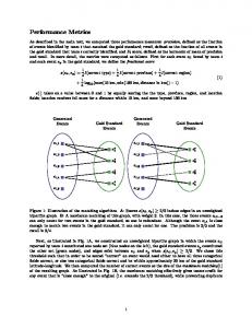
II. General System Structure This section introduces an exemplary adaptive flight control system, which will be later used to demonstrate the metrics introduced in the coming sections. The general system structure is depicted in Figure 1 and will be used for the computation of simulation-based metrics. Starting from this model, a simplified system representation for the adaptive control law design and the analytical metrics computation will be derived. The general system structure in Figure 1 comprises linear models of the aircraft motion, the structural modes, the actuators, the structural filters and the sensors. Furthermore, time delays due to delay
Structural Filter
EFG >
Transmission & Computers
C
A
Actuators
Structural Modes
Sensors
Plant
Figure 1. General System Structure
3 American Institute of Aeronautics and Astronautics
D
@̅
Aircraft
Structural Modes
̅
The aircraft in Figure 1 is given by a 4-by-4 linearized longitudinal state space model: & K K 8 K ̅ = L &, M = N ;; 8O; &$K &-K
& T 8;O &, P ⋅ L M S N ;; TO; 8OO &$ &R
&* T;O P⋅N P S @̅ '?( S )̅' , TOO UVW &&+ YZ X
̅
D , ?(,
(1)
where 84[ ∈ ]O^O , _, ` 1,2 and T4,[ ∈ ]O^; , _, ` 1,2. Modeling errors due to linearization and neglected dynamics, etc. are considered by the term )̅' , D , ?(. The structural modes of the aircraft are modeled as 2nd order transfer functions at the input and the output of the aircraft with the following structure: bD
c O S 2d; 9 c S 9 O , c O S 2dO 9 c S 9 O
(2)
where 9 is the natural frequency and the damping coefficients d; e dO determine the height of the peak. The actuators are represented by 2nd order lag elements, whereas the sensors dynamics are considered to be ideal. Numerical values of this plant model may be found in Section V. Subsequently, a linear Proportional Integral (PI) f tracking controller with additional pitch damper and an augmenting adaptive controller will be derived for the above aircraft structure. The control law for the elevator deflection B C is hence given by BC
where gh is the control signal computed by the baseline controller and 7i is the control signal deriving from the adaptive augmentation. In order to avoid the excitation of structural modes, 2nd order notch filters are used to filter the control signal B C . Their structure is equivalent to the modeling of structural modes in Eq. (2) with the only difference that for a notch filter damping coefficients d; j dO are used. For the computation of the control signals, both controllers use filtered measurements AB'?( k& B f '?( &-B'?(l+ of the pitch rate &-'?( and the load factor & f '?(. The filtering of &-'?( and & f '?( is performed by 2nd order notch filters and removes measurement errors due to the structural modes. The PI baseline control law shown in Figure 2 is assumed to be designed to fulfill certain robustness and handling quality requirements and is given by:
k where o l, and & 4 is the integrator state:
gh
gh
S
7i ,
&
&
4
p
& Bf
1
q ∙ @
6@T and PM > 45°), as well as acceptable flight/handling qualities14 for the shortperiod approximation, as seen in Figure 6. Notch filters that have the same structure as the structural mode model in Eq. (2) are used to account for structural modes. The damping coefficients d; and dO were chosen to provide a notch of −8 @T at the natural frequency of the structural mode. Load Factor nZ
2.2
nZ,CM D
nZ in [g ]
2
nZ,P lant
1.8 1.6 1.4 1.2 1 0.8 0
5
10
15
20
25
30
t in [ s]
Pitch Rate q 5
0
2 in [deg ]
q in [ deg s ]
3 2 1 0
10
-2
-4
-6
-1 -2
Elevator De.ection 2
2
4
0
5
10
15
20
25
-8
30
t in [ s] Control Antecipation Parameter CAP
1
0
5
10
15
20
Overshoot
CAP in [deg]
0
Level 1 10
10
-1
0.2
Excessive
2.5
2
1.5
Acceptable
Level 3
-2
0.3
0.4
0.5
0.6
0.7
0.8
0.9
1
30
3
Level 2 10
25
t in [s] Gibson Dropback Criterion GDC
1.1
1.2
1
0
0.5
1
1.5
2
2.5
Dropback
9SP
Figure 6. Baseline Controller Performance. Starting from the baseline controller designed for nominal conditions, an adaptive augmentation according to Section II is derived to account for matched uncertainties in , and . Each of the three quantities is assumed to be known within a 30% range around their nominal value. The parameters of the adaptation law (18) have then been chosen to provide increased system performance over the baseline controller when facing uncertainties in , and . In Figure 7, the performance of the baseline controller is compared to the adaptively augmented baseline controller, when simulating the structure of Figure 1. The maneuver consists of applying three step load factor commands of 2 t, 0.5 t and 1 t at ? 2 s, ? 17 s and ? 32 s, respectively. Subfigures a), c), e) show the performance for the nominal values of , and , while Subfigures b), d), f) show the aircraft response, when and are 30% above their nominal value and is 30% below its nominal value, which corresponds to a worst-case scenario in terms of controller performance. While in nominal conditions the performance of the baseline controller is satisfactory, it clearly degrades for larger uncertainties. By virtue of the adaptive augmentation, the degradation in performance may be attenuated. 18 American Institute of Aeronautics and Astronautics
A. Robustness Metrics The robustness of the derived adaptive control system is now analyzed using several of the analytical and simulation-based robustness metrics presented in Sections III.A and IV.A. First of all, the time-delay margin is estimated using the linearization method presented in Section III.A.1. To this extent, the adaptive control system Eqs. (10), (14), (18) is considered. Furthermore, it is assumed that the control effectiveness is known to be Λ 1, so that no feed-forward adaptation is required. Since the linearization Eq. (25) depends on the true matched uncertainty Θ ,0 1 , the values of and are varied within their uncertainty ranges and for each grid point, the step response of the closed-loop system according to Eqs. (10), (14), (18) to a step command of amplitude = 1 ∙ t is simulated to obtain the equilibrium of the adaptive control system. For each of the equilibria, the linearization is performed and a time-delay margin is estimated by determining the open-loop transfer function from the closed-loop linearization Eq. (25). Using the smallest of these values, a time-delay margin of τÕ,Ö×Ø ≈ 0.64 s was estimated. Simulation of the Eqs. (10), (14), (18) with this time-delay do however exhibit unstable behavior. This result comes as no surprise and highlights that the linearization method is indeed only able to analyze the robustness of the adaptive control in the vicinity of the equilibrium. Next, the time-delay margin of the adaptive control system for the full system structure given by Figure 1 is determined using simulations. Again, the values of , and are varied within their uncertainty ranges and for each grid point, the largest tolerable time-delay