remote sensing Article
Performance Assessment of Tailored Split-Window Coefficients for the Retrieval of Lake Surface Water Temperature from AVHRR Satellite Data Gian Lieberherr 1,2, * 1 2 3
*
ID
, Michael Riffler 3 and Stefan Wunderle 1,2
Institute of Geography, University of Bern, Hallerstrasse 12, CH-3012 Bern, Switzerland;
[email protected] Oeschger Centre for Climate Change Research, University of Bern, Falkenplatz 16, CH-3012 Bern, Switzerland GeoVille Information Systems and Data Processing GmbH, 6020 Innsbruck, Austria;
[email protected] Correspondance:
[email protected]; Tel.: +41-31-631-8554
Received: 18 October 2017; Accepted: 14 December 2017; Published: 20 December 2017
Abstract: Although lake surface water temperature (LSWT) is defined as an essential climate variable (ECV) within the global climate observing system (GCOS), current satellite-based retrieval techniques do not fulfill the GCOS accuracy requirements. The split-window (SW) retrieval method is well-established, and the split-window coefficients (SWC) are the key elements of its accuracy. Performances of SW depends on the degree of SWC customization with respect to its application, where accuracy increases when SWC is tailored for specific situations. In the literature, different SWC customization approaches have been investigated, however, no direct comparisons have been conducted among them. This paper presents the results of a sensitivity analysis to address this gap. We show that the performance of SWC is most sensitive to customizations for specific time-windows (Sensitivity Index SI of 0.85) or spatial extents (SI 0.27). Surprisingly, the study highlights that the use of separated SWC for daytime and night-time situations has limited impact (SI 0.10). The final validation with AVHRR satellite data showed that the subtle differences among different SWC customizations were not traceable to the final uncertainty of the LSWT product. Nevertheless, this study provides a basis to critically evaluate current assumptions regarding SWC generation by directly comparing the performance of multiple customization approaches for the first time. Keywords: LSWT; AVHRR; dual channel; split-window coefficients; thermal infrared; radiative transfer
1. Introduction 1.1. Accuracy of Satellite-Based Acquisition of Lake Water Temperature Measurements Lake surface water temperature (LSWT) has been identified by the global climate observing system (GCOS) as one of the essential climate variables (ECV) [1]. Consequently, there is ongoing interest to monitor this variable to detect long-term trends. Water temperature is not only an important ecological parameter in lacustrine eco-systems [2], it can also serve as a proxy for detection of local climate change [3]. Studies have revealed global warming trends for LSWT within different climate zones (e.g., [4,5]), and there is evidence that indications of climate change are sometimes even stronger within lake than in air temperature records (e.g., [6,7]). To further explore these trends on a continental or even a global scale, there is a need to generate accurate and homogeneous LSWT time series from different climatic regions. The World Meteorological Organisation (WMO) recommends that time series prepared for climate studies should ideally consist of data records that exceed 30 years. Traditionally, lake water temperature monitoring is based on in-situ measurements acquired from individual lakes. Thus, the availability of measurement data is often restricted to point-based locations, Remote Sens. 2017, 9, 1334; doi:10.3390/rs9121334
www.mdpi.com/journal/remotesensing
Remote Sens. 2017, 9, 1334
2 of 22
and limited to a specific duration. Moreover, a range of measurement methods have been applied to retrieve these in-situ records (e.g., based on the use of different instruments, defined measurement depths, etc.). This heterogeneity in terms of data coverage and retrieval methods hampers the detection of climate signals within individual lakes and even more notably when comparing climate signals associated with different lakes. Satellite-based temperature measurements overcome these limitations. The data is spatially and temporally homogeneous and is acquired with a consistent measurement method across the defined regions of interest. They can be used to create independent time-series datasets, to complement existing in-situ temperature records or to merge different datasets by serving as a relatively more robust and extensive baseline record. The advanced very high-resolution radiometer (AVHRR) sensors provide thermal infrared (TIR) data at two separate wavelengths, from NOAA-satellites since the early 1980s and from EUMSAT MetOp-satellites since 2002. Consequently, time series data that spans more than 30 years is available. The potential to generate extensive and temporally homogeneous time series provides motivation to further improve AVHRR data processing methods. However, the accuracy of LSWT retrieval from raw satellite data depends on many factors. Many sources along the processing chain contribute to the aggregated uncertainty associated with the final data product [8]. The retrieval method itself (accounting for atmospheric correction), hardware/sensor-related uncertainties, and uncertainties from different sources along the processing chain (cloud screening, geolocation, resampling, and calibration) are all known sources of contribution. Furthermore, the accuracy of LSWT retrieval from satellite data strongly depends on the characteristics of the target lake defined by its local properties (climate, latitude, altitude) and its morphology (depth, size, flow dynamics) [9,10]. Under optimal conditions and with careful post-processing, an accuracy of 90% cloud coverage over the NSC, an approximately 50% probability of >90% cloud coverage over the NSC, whereas around 15% over whereas around 15% over Greece. Temperature retrieval based on TIR radiation requires clear sky Greece. Temperature retrieval on TIRwith radiation sky observations. Sincethey clouds observations. Since clouds based are opaque respectrequires to TIR clear wavelengths, and therefore are are opaque with respect to TIR wavelengths, and therefore they are excluded from the matchup data. excluded from the matchup data.
Figure 1. The five areas where the sensitivity analysis was performed.
Figure 1. The five areas where the sensitivity analysis was performed.
Remote Sens. 2017, 9, 1334
5 of 22
Remote Sens. 2017, 9, 1334 Remote Sens. 2017, 9, 1334
5 of 22 5 of 22
The extends over over Norway Norway and andSweden Swedenininthe thewest, west,Finland Finlandininthe thecenter center and Russia The NSC NSC site site extends and Russia in The NSC site extends over Norway and Sweden in the west, Finland in the center and Russia in at in the east. The topography is rather flat and homogeneous for the majority of the region. However, the east. The topography is rather flat and homogeneous for the majority of the region. However, theat east. The topography isthe rather flat and mountains homogeneous for the of the region. However, atact the north-western edge the Norwegian mountains elevates to about 1500 m a.s.l.; these features the north-western edge Norwegian elevates tomajority about 1500 m a.s.l.; these features theact north-western edge the Norwegian mountains elevates to about 1500 m a.s.l.; these features act as an orographic barrier against prevailing westerly weather conditions. The region is generally as an orographic barrier against prevailing westerly weather conditions. The region is generally as colder an orographic against prevailing weather The region is generally and than other to and to influence of colder and dryer dryerbarrier than the the other regions regions due duewesterly to its its latitude latitude andconditions. to the the decreasing decreasing influence of the the Gulf Gulf colder and dryer than the other regions due to its latitude and to the decreasing influence of the Gulf Stream. Even though the total column of water vapor in the atmosphere is low and stable (Figure Stream. Even though the total column of water vapor in the atmosphere is low and stable (Figure 2), 2), Stream. Evenhas though therate total of water vapor in the atmosphere is low and stable (Figure 2), the aa high of cloud which significantly reduces number of satellite the region region has high rate ofcolumn cloud cover, cover, which significantly reducesthe the number of suitable suitable satellite theobservations region has a(Figure high rate 3). observations (Figure 3).of cloud cover, which significantly reduces the number of suitable satellite observations (Figure 3).
Figure 2. 2. Average Averageof ofthe the total total content content of of water water vapor vapor over over Europe Europefor forthe theperiod period2000–2012. 2000–2012. (ECMWF (ECMWF Figure Figure 2. Average of theset total content of water vapor over Europe for the period 2000–2012. (ECMWF ERA-INTERIM data [30]). ERA-INTERIM data set [30]). ERA-INTERIM data set [30]).
Figure 3. Cumulative density function (CDF) of cloud cover for the five regions. P (TCC) is the Figure 3. Cumulative function (CDF) of cloud (TCC) cover rate for the five regions. P (TCC) is the probability to occurdensity thatdensity a certain total cloud is (Data: ECMWF ERAFigure 3. Cumulative function (CDF)cover of cloud cover forexceeded. the five regions. P (TCC) is probability to occur that a certain total cloud cover (TCC) rate is exceeded. (Data: ECMWF ERAINTERIM [30] 2000–2012). the probability to occur that a certain total cloud cover (TCC) rate is exceeded. (Data: ECMWF INTERIM [30] 2000–2012). ERA-INTERIM [30] 2000–2012).
The SSC site extends over Norway, Sweden and Denmark, and parts of the Baltic Sea. The The SSC site extends over Norway, Sweden and Denmark, and the parts of the Baltic Sea. The topography is flat towards the south-east and mountainous towards north-west, with elevations The SSC site extends over Norway, Sweden and towards Denmark, and parts of theelevations Baltic Sea. topography is flat towards the south-east and mountainous the north-west, with reaching 2600 m a.s.l. The topographic features form an orographic barrier like that observed in the The topography is flat towards the south-east and mountainous towards the like north-west, with elevations reaching 2600 m a.s.l. The topographic features form an orographic barrier that observed in the NSC site, resulting in dryer conditions over Sweden. On the other hand, the notable influence of the NSC site, resulting in dryer conditions over Sweden. On the other hand, the notable influence of the
Remote Sens. 2017, 9, 1334
6 of 22
reaching 2600 m a.s.l. The topographic features form an orographic barrier like that observed in the NSC site, resulting in dryer conditions over Sweden. On the other hand, the notable influence of the Gulf Stream leads to a generally warmer and more humid climate over the whole region. The cloud cover rate is, as for NSC, high and consequently reduces the number of clear sky observations (Figure 3). The EEU site extends mainly over Poland, Hungary, Slovakia, Romania and Ukraine. The hilly and mountainous topography is dominated by the Carpathian ridge, and the highest elevations reach over 2600 m a.s.l. The continental climate is characterized by pronounced seasonal patterns, especially with respect to temperature differences. The atmosphere is generally drier and less influenced by short term weather dynamics induced by the moisture influx of the sea. The ALP site extends over Germany, France, Italy, Austria and Switzerland. The pronounced topography ranges from a few meters a.s.l. in the Po-Basin to over 4000 m a.s.l. in the Alps. The region is characterized by the alpine ridge, which acts as a strong orographic barrier that separates the north and the south into two distinct climatic regions. Whereas the north is generally colder and has a slightly more continental climate, the south is strongly influenced by the warm Mediterranean Sea and its important moisture influx to the atmosphere (Figure 2). The GRE site extends over the Balkans, southern Italy, Greece, Bulgaria and parts of the Mediterranean Sea. It is the most heterogeneous one of the five regions, not only in terms of topography but also in terms of land/water transition. The hilly yet mountainous topography on the main land reaches elevations of over 2900 m a.s.l. in the Olympus mountain range, and it includes parts of the Ionian Sea, the Aegean Sea and a large quantity of small islands. The warm Mediterranean climate provides a constant supply of water vapor from the sea, along with an increased storage capacity for water vapor in the atmosphere. The combined effect results in elevated absolute humidity rates (Figure 2), and relatively low cloud coverage over the GRE region (Figure 3). 2.2. Generation of Matchup Data To generate the matchup data, the fast radiative transfer model for TIROS operational vertical sounder (RTTOV) v.11 [31] was used. The model is known to be capable of producing highly accurate results efficiently. The RT-model was fed with atmospheric profile data extracted from the ECMWF ERA-INTERIM reanalysis data ([30]). The ERA-INTERIM dataset is a global atmospheric reanalysis dataset with spatial resolution of about 80 km grid cells and a temporal resolution of 6 h. The dataset was designed to be used in climate studies (i.e., long-term stability), and has a temporal extent that covers the entire period where AVHRR-2 and -3 data is available (i.e., 1979 to the present day). For this study, the atmospheric profiles and ground parameters were extracted for every grid cell within the five regions at a six-hour time step for a period of four years (2002–2005). This produced meteorological dataset with over 3.5 M atmospheric profiles and corresponding ground data. For each of these atmospheric profiles, the RT-model was run 40 times to include satellite view zenith angles (VZA) between 0◦ and 60◦ and surface temperatures between −5 ◦ C and 35 ◦ C. A total of over 142 M radiative transfer model runs were conducted to create the match-up database, with a distinct matchup pair being produced with the completion of each run. 2.3. Validation Data The final validation was performed for a four-year period (2004–2007), by comparing satellite-derived LSWT with in-situ measurements at Lake Constance and Lake Geneva. Pre-processed AVHRR data from NOAA-17 archived at the Remote Sensing Group of the University of Bern [32] was used for the validation. The derived LSWT product was compared to hourly in-situ measurements from Lake Geneva and Lake Constance for the whole test period. The measurements made at Lake Geneva were recorded at a location (46.458◦ N, 6.399◦ E) about 100 m from the shore and 1 m below the water surface. The measurements at Lake Constance were taken in the Lindau Harbor (47.544◦ N, 9.685◦ E), at a depth of 0.5 m.
Remote Sens. 2017, 9, 1334
7 of 22
3. Method 3.1. Sensitivity Analysis For the sensitivity analysis (SA), the ‘one-at-a-time’ or ‘local’ approach (e.g., [33]) was used such that only one input variable was modified at a time while the others remained constant at their baseline values. The initially modified input variable is then reset to its baseline value, and the same procedure is repeated for each of the other input variables. With this approach, any observed change in the output can be ascertained to the specific input variable that was modified in isolation. A quantitative comparison of the impacts of the input variables is possible as each variable is explored from the same starting point (baseline). To quantify the performance of the variables of interest with the SA, the intrinsic error of the SWC is used as performance indicator. The intrinsic error is equal to the regression error, which is the standard deviation (SD) between the matchup data and the mathematical model (Equation (1) parametrized with the SWC). Furthermore, a sensitivity index (SI) is computed for each parameter. The SI is defined as the difference between the largest and the smallest intrinsic error, scaled to the baseline value. For each SWC customization approach, a different sub-set of the matchup data base was chosen to regress the coefficients. The filter to select the matchup data used for the coefficients regression translates into the parameter space during which is explored during the SA. The SA is performed on the six parameters expected to be the most influential; the ranges of values associated with each parameter is summarized in Table 1. We also assume that all of the input variables are independent, and any correlations are considered to be negligible. While this assumption is not entirely true, the potential correlations are considered to be weak, and will not significantly affect the outcome of the SA. Table 1. Overview of the parameters and the associated range of values explored with the sensitivity analysis. Baseline values are bold. Parameter
Units
Time window Spatial radius VZA range Sfc Temperature TCWV Day/night separation
[days] [km] n bins n bins n bins true/false
1
2
4
7
14
30 50 1 1 1 false
90 90 2 2 2 true
180 125 4 4 4
360 200 10 10 10
720 300
400
550
The baselines for the time window and the spatial radius are chosen based on the results of a preliminary analysis, which was conducted, but excluded from this paper for the sake of brevity. The baseline for the view zenith angle was chosen based on values reported in the literature (see below), and the baseline values for the other variables is set to ‘all’. This effectively includes all realistic values without constraints. The spatial extent (radius R in km) is defined as the region where the same set of coefficients can be applied without substantial loss in accuracy. If such a region is circular, the size of the region can be expressed by its radius R (i.e., distance from the center to the edge of the circle). The SA explores different spatial extents within R = [0, 500] km. While the maximum radius of 500 km is associated to a rather small region, the preliminary analysis showed that errors stabilized for distances exceeding 1000 km. Consequently, Rmax was set to 550 km. The baseline value for the region size was fixed at R = 50 km, which was identified as a good trade-off from the results of the preliminary analysis. The time window is defined as the interval (in days) within which a set of coefficients remains valid without substantial loss in accuracy; it is dependent on the stability of the atmospheric conditions over time. Time window intervals between one day and two years were investigated. Based on the results of the preliminary analysis, a baseline value of 30 days was selected.
Remote Sens. 2017, 9, 1334
8 of 22
The view zenith angle (VZA) is an important factor that affects the accuracy of coefficients. It defines the length of the path a signal must travel through the atmosphere, and also the strength of the emitted signal (i.e., directional emissivity). These effects are supposed to be accounted for by the formulation of the retrieval method (i.e., the VZA dependent term in Equation (1)). However, a significant decrease in accuracy can be observed at larger VZAs around 45–60 degrees. The VZA parameter is represented by the number of equal sized bins with which the VZA range between 0 and 60 degrees is divided. Thus, three VZA bins means that we compute three sets of coefficients, one of each that is applicable for lower, medium, and high VZA, respectively. The VZA is not limited to a defined threshold; the whole range of available data from nadir to about 58 degrees is explored. The baseline is using only one bin, meaning that there is only one set of coefficients covering the whole range of VZA. The surface temperature (Tsfc) is the temperature of the emitting body. It determines the strength of the emitted signal at the earth’s surface and also influences the emissivity itself [34]. Similar to the VZA limit, the parameter represents the number of bins that is applied to split the range; the result is then applied to separate coefficients. The baseline is one Tsfc bin, which means that a single set of coefficients covers the whole range of Tsfc values. The water vapor content (total column of water vapor, TCWV) in the atmosphere absorbs electromagnetic radiation in the TIR. Consequently, its influence on the coefficients quality is of interest. Like for the VZA bins and the Tsfc bins, the parameter defines the number of distinct ranges into which the range of possible water vapor content values is divided. The baseline is one TCWV bin, meaning that there is only one set of coefficients covering the whole range of TCWV values. The time of the day is used to generate specific coefficients for day-time and night-time temperature retrieval. The ERA-INTRIM reanalysis dataset provides data four times a day at 0 h, 6 h, 12 h and 18 h. Two variations with and without the separation of day/night coefficients were set up in this study. Day and night-time is defined by the sun zenith angle, where five degrees over the horizon is defined as daytime and 5 degrees below the horizon is considered as night-time. The twilight period in between the two defined periods of time is excluded in this study. The variant without distinction between day and night was selected as the baseline. 3.2. Validation Based on the results from the sensitivity analysis, different sets of coefficients are generated and applied to a set of satellite data. Thus, for each set of SWC, a LSWT time-series is derived, and compared to the available in-situ data collected from Lake Geneva and Lake Constance. Both temporal and spatial matches were identified to compare the two types of measurements. From each satellite scene, the average of all pixel values within a 5 km radius around the in-situ measurement location is taken to calculate the satellite-based LSWT value. This value is then compared to the in-situ measurement with the closest time stamp to the satellite overpassing time, and within a 2 h temporal window. 3.3. Uncertainty Propagation Analysis The LSWT processing chain includes many sources of uncertainties. These uncertainties are propagated and aggregated in the final LSWT product. To estimate the influence and the relevance of the SWCs’ intrinsic uncertainty, a model that quantifies the amount of error that is propagated throughout the processing chain is needed. In this study, the uncertainty analysis is limited to the relationship between the total amount of uncertainty and the SWCs’ intrinsic uncertainty. Therefore, the error propagation model can be simplified by assuming that only the combination two sources contribute to the total uncertainty, namely the SWCs’ intrinsic uncertainty (σSWC ) and the auxiliary uncertainty (σaux ). The latter is a factor that combines the cumulative effect of all uncertainties in the processing chain, excluding the SWCs’ intrinsic uncertainty. To further simplify the problem, the two sources are assumed to independent from each other, and having a Gaussian uncertainty distribution.
Remote Sens. 2017, 9, 1334
9 of 22
A simple error propagation model can be applied under the aforementioned assumptions; the model is described by Equation (2) [35,36], and is applied to estimate the influence of the SWCs’ intrinsic uncertainty on the total uncertainty. σtot =
q
σSWC 2 + σaux 2
(2)
σtot Total uncertainty of the LSWT product; σSWC uncertainty issued from the SWCs regression; σaux uncertainty from all other sources expect from the SWCs. From the sensitivity analysis, the range of expected SWC intrinsic uncertainty values is known, and the total uncertainty is determined from the LSWT product. Hence, the influence of SWCs’ intrinsic uncertainty on the total uncertainty of any validated LSWT product can be determined. Likewise, this can also be determined for data derived from other sensors using the same retrieval method. 4. Results 4.1. Results of the Sensitivity Analysis 4.1.1. Region Size The effect of region size on the SWC depends on the study region. In general, the intrinsic error associated with the GRE site is the highest, followed by the error associated with the EEU, ALP sites, and lowest in the SSC and NSC sites (Figure 4). This observation is expected, as regions with higher temperatures are supposed to have more dynamic atmospheric conditions, which are linked to higher SWC uncertainties. However, the sensitivity of SWC to region size is strongest in NSC (Sensitivity Index, SI of 0.51), followed by the ALP (0.40), and GRE (0.31). SWC sensitivity to region size is limited in both the EEU (0.05) and SSC (0.06) sites; the results are summarized in Table 2. Table 2. Overview of the intrinsic errors (in degrees of K) for each region, with respect to variable radius values. The sensitivity index (SI) is defined as the difference between the largest and the smallest intrinsic error, scaled to the baseline value (i.e., radius of 50 km). SI (-)
ALP SSC NSC EEU GRE AVG
0.40 0.06 0.51 0.05 0.31 0.27
Intrinsic Error (K) with Changing Radius 550 km
400 km
300 km
200 km
125 km
90 km
50 km
0.150 0.105 0.088 0.168 0.201 0.143
0.148 0.104 0.083 0.167 0.199 0.140
0.140 0.101 0.079 0.167 0.193 0.136
0.131 0.101 0.075 0.168 0.180 0.131
0.124 0.101 0.069 0.168 0.165 0.125
0.120 0.100 0.067 0.167 0.162 0.123
0.108 0.099 0.058 0.160 0.154 0.116
For regions with intrinsic errors that were identified to be more sensitive to changes in radius values (NSC, ALP, GRE), a strong increase in intrinsic error for lower radii up to about 200 or 300 km is observed; after this range of values, the intrinsic error tends to stabilize (Figure 4). For the EEU region, the increase in the sensitivity of intrinsic errors to changes in radius values occurs between 50 km to 90 km, then stabilizes for larger region sizes. For the SSC region, the intrinsic error remains stable over the whole range of tested radius values.
Remote Sens. 2017, 9, 1334
10 of 22
Remote Sens. 2017, 9, 1334
10 of 22
Remote Sens. 2017, 9, 1334
10 of 22
Figure 4. For each of the five regions: Evolution of the SWC’s intrinsic error, when increasing the
Figure 4. For each of the five regions: Evolution of the SWC’s intrinsic error, when increasing the spatial radius (distance from the region’s center) where the SWC are considered to be valid. spatial radius (distance the regions: region’sEvolution center) where SWCintrinsic are considered to be valid. the Figure 4. For each offrom the five of thethe SWC’s error, when increasing
4.1.2.spatial Time radius Window Size from the region’s center) where the SWC are considered to be valid. (distance
4.1.2. Time Window Size
For all regions, SWC are very sensitive to the time window size. In Table 3, it can be observed 4.1.2. Time Window Size that SI for theSWC regions 0.77 intoEEU to window 1.00 in NSC. For the all regions, arevary veryfrom sensitive the up time size. In Table 3, it can be observed that For all regions, SWC are very sensitive to the time window the SI for the regions vary from 0.77 in EEU up to 1.00 in NSC. size. In Table 3, it can be observed Table 3. Overview of vary the Intrinsic errors (in degree K) for each region and time window. The that the SI for the regions from 0.77 in EEU up to 1.00 in NSC. sensitivity index (SI) is defined as the difference between the largest and the smallest intrinsic error,
Table 3. Overview of the Intrinsic errors (in degree K) for each region and time window. The sensitivity scaled baselineofvalue 30-day time(in window). Table to 3. the Overview the (i.e., Intrinsic errors degree K) for each region and time window. The index (SI) is defined as the difference between the largest and the smallest intrinsic error, scaled to the sensitivity index (SI) is defined as the difference between the largest and the smallest intrinsic error, SI (-)(i.e., 30-day time window). Intrinsic Error (K) with Changing Time-Window baseline value scaled to the baseline (i.e., 30-day time 90-day window).30-day 720-day value 360-day 180-day
ALP SSC NSC ALP EEU ALP SSC GRE SSC NSC AVG NSC EEU
0.80 SI (-) SI (-) 0.87 1.00 0.80 0.77 0.80 0.87 0.78 0.87 1.00 0.85 1.00 0.77
0.129 0.119 720-day 720-day 0.080 0.129 0.178 0.129 0.119 0.175 0.119 0.080 0.136 0.080 0.178
0.125 0.115 360-day 360-day 0.079 0.125 0.178 0.125 0.115 0.173 0.115 0.079 0.134 0.079 0.178
14-day 7-day 4-day 0.124 0.119 0.108 0.096 0.086 0.075 Intrinsic Changing Time-Window IntrinsicError Error(K) (K)with with Changing Time-Window 0.114 0.109 0.099 0.090 0.076 0.067 180-day 90-day 30-day 14-day 7-day 4-day 180-day 90-day 30-day 14-day 7-day 4-day 0.077 0.070 0.058 0.052 0.048 0.037 0.124 0.119 0.108 0.096 0.086 0.075 0.179 0.177 0.160 0.141 0.118 0.092 0.124 0.119 0.108 0.096 0.086 0.075 0.114 0.109 0.099 0.090 0.076 0.067 0.174 0.167 0.154 0.141 0.121 0.100 0.114 0.077 0.109 0.070 0.099 0.058 0.090 0.052 0.076 0.048 0.067 0.037 0.134 0.129 0.116 0.104 0.090 0.074 0.077 0.179 0.070 0.177 0.058 0.160 0.052 0.141 0.048 0.118 0.037 0.092
2-day 0.061 0.042 2-day 2-day 0.029 0.061 0.062 0.061 0.042 0.073 0.042 0.029 0.054 0.029 0.062
1-day 0.043 0.033 1-day 1-day 0.022 0.043 0.056 0.043 0.033 0.055 0.033 0.022 0.042 0.022 0.056
EEU 0.178 0.178 0.179 0.062 0.055 0.056 GRE 0.77 0.78 0.175 0.173 0.174 0.177 0.167 0.160 0.154 0.141 0.141 0.118 0.121 0.092 0.073 The main component of the intrinsic error accumulates within the first0.100 two weeks GRE 0.175 0.173 0.174 0.073(Figure 0.0555), AVG 0.78 0.85 0.136 0.134 0.134 0.167 0.129 0.154 0.116 0.141 0.104 0.121 0.090 0.100 0.074 0.054 0.042 where intrinsic0.134 error increases from of 0.042 K (1 day)) to 0.1040.054 K (14 days). AVG the average 0.85 0.136 0.134 0.129 an average 0.116 0.104 0.090 0.074 0.042
Persistent weather remain over Europe days(Figure up to two The main synoptic component of thesystems intrinsictypically error accumulates within thefrom first several two weeks 5), weeks. Those short-term changes in the atmosphere accountoffor main where the average intrinsic error increases from an average 0.042 K sources (1 day))of toSWC 0.104uncertainties. K (14 days). The main component of the intrinsic error accumulates within the first two weeks (Figure 5), Persistent synoptic weather systems typically remain over Europe from several days up to two where the average intrinsic error increases from an average of 0.042 K (1 day)) to 0.104 K (14 days). weeks. Those short-term changes in the atmosphere account for main sources of SWC uncertainties.
Figure 5. For each of the five regions: Evolution of the SWC’s intrinsic error, when increasing the timewindow within which the SWC are considered to be valid. Figure 5. For each of the five regions: Evolution of the SWC’s intrinsic error, when increasing the time-
Figure 5. Forwithin each which of thethe five regions: Evolution of valid. the SWC’s intrinsic error, when increasing the window SWC are considered to be time-window within which the SWC are considered to be valid.
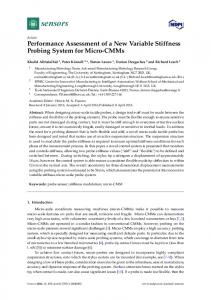
source of uncertainty. The change in uncertainty appears to plateau when the time window size increases beyond approximately one year (Figure 5). A 721-day time window is associated with almost the same amount of intrinsic error (0.136 K) as a 180-day time window size (0.134 K). The shortest time window that was investigated in the study corresponds to one full day; the Remote Sens. 2017, 9, 1334 11 of 22 effects of day/night cycle were not captured as a result. 4.1.3.Persistent View Zenith Angleweather (VZA) systems typically remain over Europe from several days up to two synoptic weeks. Those short-term changes in the atmosphere account for main sources of SWC uncertainties. We expected a rather stable behavior to be associated with changing the VZA parameter, since Another significant increase in uncertainties can be observed when the time window increases it is integrated in the retrieval method (Equation (1)). In particular, the method was designed to from 30 to 180 days, which corresponds to increases from 0.116 K to 0.134 K on average. Based on this handle the whole range of possible VZA values with the same set of coefficients. However, upon observation, the seasonal variability in the atmosphere seems to be significant and an important source further inspection of the individual intrinsic errors associated with each resultant subrange after of uncertainty. splitting the full range of VZA values into 10 bins (Figure 6), it is evident that for VZA of more than The change in uncertainty appears to plateau when the time window size increases beyond 35 to 45 degrees, the intrinsic error increases significantly over all of the investigated regions. approximately one year (Figure 5). A 721-day time window is associated with almost the same amount Figure 7 highlights only a slight increase in the overall accuracy with respect to how the VZA of intrinsic error (0.136 K) as a 180-day time window size (0.134 K). range is divided into several small sub-ranges with own coefficients. Strong sensitivity to changes in The shortest time window that was investigated in the study corresponds to one full day; the VZA is detected in the ALP site with an SI of 0.2 and the uncertainty is reduced from 0.108 K to the effects of day/night cycle were not captured as a result. 0.086 K (Table 4). In the NSC (SI 0.15), SSC (SI 0.12), and GRE (SI 0.07) sites, the reduction in uncertainty is already very low, whereas there is no significant improvement observed over the EEU 4.1.3. View Zenith Angle (VZA) (SI 0.02) site. We expected rather that stablethis behavior to be changing the VZA parameter, sincebe it It should bea noted increase is associated unrelated with to any confounding effects that may is integrated the retrieval method (EquationWhile (1)). In particular, the method waswhen designed to handle attributed toinpixel overlapping or blurring. this explanation is relevant working with the whole range of possible VZA values with the same set of coefficients. However, upon pixels from real satellite images, it is not applicable with respect to simulated pixels. The latter further remain inspection of the individual intrinsic errors with each resultant subrange splitting the perfect individual dots for the full range of associated VZA values. Consequently, this increaseafter in uncertainty at full range of VZA values into 10 bins (Figure 6), it is evident that for VZA of more than 35 to 45 degrees, larger VZA values is related to other mechanisms not considered in the split-window equation the intrinsic error increases significantly over all of the investigated regions. (Equation (1)).
Figure 6. 6. Intrinsic error error from from each each of of the the 10 individually individually tailored tailored SWC SWC of of the the variant variant with with 10 10 VZA VZA bins bins Figure variant. On On the the x-axis x-axis have have the the VZA VZA values values of of the the bin bin centers. centers. variant.
Figure 7 highlights only a slight increase in the overall accuracy with respect to how the VZA range is divided into several small sub-ranges with own coefficients. Strong sensitivity to changes in the VZA is detected in the ALP site with an SI of 0.2 and the uncertainty is reduced from 0.108 K to 0.086 K (Table 4). In the NSC (SI 0.15), SSC (SI 0.12), and GRE (SI 0.07) sites, the reduction in uncertainty is already very low, whereas there is no significant improvement observed over the EEU (SI 0.02) site. It should be noted that this increase is unrelated to any confounding effects that may be attributed to pixel overlapping or blurring. While this explanation is relevant when working with pixels from real satellite images, it is not applicable with respect to simulated pixels. The latter remain perfect individual dots for the full range of VZA values. Consequently, this increase in uncertainty at larger VZA values is related to other mechanisms not considered in the split-window equation (Equation (1)).
Remote Sens. 2017, 9, 1334
12 of 22
Remote Sens. 2017, 9, 1334
12 of 22
Remote Sens. 2017, 9, 1334
12 of 22
Figure 7. For each of the five regions: Evolution of the SWC’s intrinsic error, when increasing the
Figure 7. For each of the five regions: Evolution of the SWC’s intrinsic error, when increasing the number of VZA bins, for which individually tailored coefficients are generated. number of VZA which tailored coefficients are generated. Figure 7. Forbins, each for of the fiveindividually regions: Evolution of the SWC’s intrinsic error, when increasing the Table 4.of Overview of for thewhich Intrinsic errors (in degree for each region and explored number of VZA number VZA bins, individually tailoredK)coefficients are generated. The sensitivity (SI) errors is defined as the difference between and number the smallest of theindex Intrinsic (in degree K) for each regionthe andlargest explored of VZA Tablebins. 4. Overview Table 4. Overview of the Intrinsic errors (in degree K) for each region and explored number of VZA intrinsic error, scaled to the baseline value (i.e., 1 bin). bins. The sensitivity index (SI) is defined as the difference between the largest and the smallest intrinsic Thetosensitivity index (SI) is defined the difference between the largest and the smallest error,bins. scaled the baseline value 1 bin).asError SI (-)(i.e.,Intrinsic (K) with Changing VZA Bins
intrinsic error, scaled to the baseline value (i.e., 1 bin). 1 bin 2 bins 4 bins 10 bins (-) Intrinsic Error with Changing VZA Bins ALP SI 0.20 0.108 0.096 0.089 0.086 SI (-) Intrinsic Error (K)(K) with Changing VZA Bins
SSC 0.12 1 bin 10.099 bin NSC 0.20 0.15 0.058 ALP 0.108 ALP 0.20 0.108 EEU 0.12 0.02 0.160 0.12 0.099 SSCSSC 0.099 GRE 0.15 0.07 0.154 NSC 0.15 0.058 NSC 0.058 AVG 0.02 0.11 0.116 EEU 0.160 EEU 0.02 0.160 GRE 0.154 GRE 0.07 0.07 0.154 4.1.4. Total ColumnAVG of Water Vapor (TCWV) 0.116 AVG 0.11 0.11 0.116
2 bins 40.090 4 bins 20.094 bins bins 0.053 0.051 0.096 0.089 0.096 0.089 0.160 0.094 0.0900.090 0.094 0.159 0.149 0.053 0.0510.051 0.053 0.145 0.110 0.160 0.107 0.160 0.1590.159 0.149 0.1450.145 0.149 0.110 0.1070.107 0.110
0.087 10 bins 10 bins 0.049 0.0860.086 0.157 0.0870.087 0.142 0.0490.049 0.104 0.1570.157 0.1420.142 0.1040.104
8 and Table 5 show that dividing the water vapor range into subranges with tailored 4.1.4. Figure Total Column of Water Vapor (TCWV)
4.1.4.coefficients Total Column Watereffect Vapor has aofsimilar in (TCWV) all regions. The sensitivity is the highest in the EEU site (SI 0.19), and Figure it is8also the largest absolute of error ranging from aboutwith 0.16–0.13 K. 8 associated and Table 5 show that dividing thereduction water range into subranges tailored Figure and Table 5 with show that dividing the water vapor vapor range into subranges with tailored On the contrary, the lowest sensitivity (SI 0.13)The andsensitivity the lowest is absolute reduction ofEEU errorsite from about coefficients has a similar effect in all regions. the highest in the (SI 0.19), coefficients has a similar effect in all regions. The sensitivity is the highest in the EEU site (SI 0.19), and it 0.06–0.05 K isassociated observed with over the NSC site, where the moisture content and the overall intrinsic error and it is also largest absolute reduction of error ranging from about 0.16–0.13 K. is also associated with the largest absolute reduction of error ranging from about 0.16–0.13 K. On the is also the lowest. On the contrary, the lowest sensitivity (SI 0.13) and the lowest absolute reduction of error from about contrary, the lowest sensitivity (SI 0.13) and the lowest absolute reduction of error from about 0.06–0.05 K 0.06–0.05 K is observed over the NSC site, where the moisture content and the overall intrinsic error is observed over the NSC site, where the moisture content and the overall intrinsic error is also the lowest. is also the lowest.
Figure 8. For each of the five regions: Evolution of the SWC’s intrinsic error, when increasing the number of TCWV bins for which individually tailored coefficients are generated.
Figure 8. For each of the five regions: Evolution of the SWC’s intrinsic error, when increasing the
Figure 8. For each of the five regions: Evolution of the SWC’s intrinsic error, when increasing the number of TCWV bins for which individually tailored coefficients are generated. number of TCWV bins for which individually tailored coefficients are generated.
Remote Sens. 2017, 9, 1334
13 of 22
Remote Sens. 2017, 9, 1334
13 of 22
Table 5. Overview of the Intrinsic errors (in degree K) for each region and explored number of TCWV bins. The sensitivityofindex (SI) is defined difference the largest and thenumber smallestofintrinsic Table 5. Overview the Intrinsic errors as (inthe degree K) forbetween each region and explored TCWV error, scaled to the baseline value (1 bin). bins. The sensitivity index (SI) is defined as the difference between the largest and the smallest
intrinsic error, scaled to the baseline value (1 bin). SI (-) Intrinsic Error (K) with Changing TCWV Bin SI (-) Intrinsic Error (K) with Changing TCWV Bin 1 bin 2 bins 4 bins 10 bins 1 bin 2 bins 4 bins 10 bins ALP 0.17 0.108 0.105 0.099 0.090 ALP 0.17 0.108 0.105 0.099 0.090 SSC 0.16 0.099 0.097 0.091 0.083 SSC 0.16 0.099 0.097 0.091 0.083 NSC 0.13 0.058 0.058 0.057 0.051 NSC 0.13 0.058 0.058 0.057 EEU 0.19 0.160 0.155 0.145 0.0510.131 EEU 0.19 0.160 0.1550.148 0.1450.142 0.1310.127 GRE 0.18 0.154 GRE 0.18 0.154 0.1480.113 0.1420.107 0.1270.096 AVG 0.16 0.116 AVG 0.16 0.116 0.113 0.107 0.096
The sensitivity is directly related to the realistic extents of the TCWV ranges occurring in the respective regions. regions. In In this this study, study,the theTCWV TCWVrange rangeofofeach eachregion regionis is subdivided into a fixed number subdivided into a fixed number of of bins. In the case of the NSC region, which is characterized by a low TCWC maxima, this results in bins. In the case of the NSC region, which is characterized by a low TCWC maxima, this narrower and more homogeneous bins that have limited impact on the the overall overall accuracy. accuracy. In In contrast, contrast, the subdivision of wider regional extents of possible moisture values into smaller subranges for other locations/ locations/sites sitesenhances enhancesthe theperformance. performance. Temperature 4.1.5. Surface Temperature Similar to the results of the investigation with with TCWV, we observe that dividing the Tsfc range into subranges has a similar effect for all regions (Figure 9). In terms of absolute change in intrinsic error, the strongest reduction is observed in the EEU site, ranging from 0.160 K to 0.134 K, while the lowest reduction is observed in the NSC site, ranging from 0.058 K to 0.049 K. In terms of SI, all the site (SI (SI 0.12), 0.12), regions have a similar sensitivity to Tsfc (EEU SI 0.17 to SSC SI 0.15), excepting the GRE site which is associated with a considerably lower sensitivity (Table 6). The observation over the latter may which is associated with a considerably lower sensitivity (Table 6). The observation over the latter be related to thetoelevated TCWV rates around the warm Mediterranean Sea, which corresponds to the may be related the elevated TCWV rates around the warm Mediterranean Sea, which corresponds high uncertainty relatedrelated to the potential effects of Tsfc bins. However, the exact cause this to thegeneral high general uncertainty to the potential effects of Tsfc bins. However, the exactfor cause remains unknown. for this remains unknown.
Figure 9. For each of the five regions: Evolution of the SWC’s intrinsic error, when increasing the Figure 9. For each of the five regions: Evolution of the SWC’s intrinsic error, when increasing the number of surface temperature bins, for which individually tailored coefficients are generated. number of surface temperature bins, for which individually tailored coefficients are generated.
Remote Sens. 2017, 9, 1334
14 of 22
Table 6. Overview of the Intrinsic errors (in degree K) for each region and explored number of surface temperature bins. The sensitivity index (SI) is defined as the difference between the largest and the smallest intrinsic error, scaled to the baseline value (1 bin). SI (-)
ALP SSC NSC EEU GRE AVG
0.16 0.15 0.16 0.17 0.12 0.15
Intrinsic Error (K) with Changing Tsfc Bins 1 bin
2 bins
4 bins
10 bins
0.108 0.099 0.058 0.160 0.154 0.116
0.101 0.093 0.055 0.150 0.147 0.109
0.097 0.089 0.052 0.144 0.143 0.105
0.090 0.084 0.049 0.134 0.135 0.099
4.1.6. Time of the Day The effect of using separated daytime and night-time SWC, instead of a general SWC, is rather low across all regions. The sensitivity is highest in the ALP and EEU sites, both with an SI of 0.11, and lowest in the GRE and SSC sites, both with an SI of 0.08 (Table 7). The highest absolute reduction in intrinsic error is to be found in the EEU region (0.160 K to 0.143 K), whereas the lowest absolute reduction is to be found in the NSC region (0.058–0.052 K). Table 7. Overview of the Intrinsic errors (in degree K) for each region and for the scenarios with and without separated day and night-time coefficients. The sensitivity index (SI) is defined as the difference between the largest and the smallest intrinsic error, scaled to the baseline value (without day/night separation). SI (-)
ALP SSC NSC EEU GRE AVG
0.11 0.08 0.10 0.11 0.08 0.10
Intrinsic Error (K) Day/Night Separation No
Yes
0.108 0.099 0.058 0.160 0.154 0.116
0.096 0.091 0.052 0.143 0.142 0.105
This result was unexpected and in contradiction to other studies (e.g., [13,19]). A possible explanation for this may be attributed to the application of a skin-to-bulk conversion that is implicit to the SWC in the other studies. In this study, only the atmospheric attenuation between the earth’s surface and the top of atmosphere was considered to generate the SWC. The study highlights this difference; while differentiating between day- and night-time situations makes sense for skin-to-bulk conversion, but it has a negligible effect on the correction of atmospheric attenuation of TIR radiation. 4.1.7. Overview Per Region When comparing the impact of the different tested parameters, the order of importance differs slightly from region to region (Figure 10). However, in all regions, the SWC are most sensitive to the time window size (average SI of 0.85). Thus, overall uncertainty can be notably minimized with the reduction of the time window size. The region size was identified to be the second most important parameter, associated with an average SI of 0.27. However, the sensitivity to the spatial extent of a region depends strongly on the region’s characteristics (e.g., topography and climatic zones). For the regions of SSC (SI 0.06) and EEU (0.05), the size of the region has almost no significance on the SWCs’ performance, whereas for the regions of NSC (SI 0.51) and ALP (SI 0.40), this parameter has a very significant effect.
Remote 2017, 9, 1334 Remote Sens.Sens. 2017, 9, 1334
15 of1522of 22
(a) NSC
(b) SSC
(c) ALP
(d) EEU
(e) GRE Figure 10. Comparison of the impact of each parameter for Northern Scandinavia (a), Southern Figure 10. Comparison of the impact of each parameter for Northern Scandinavia (a), Southern Scandinavia (b),(b), Eastern Europe Greece (e). (e).The Thered redhorizontal horizontal line represents Scandinavia Eastern Europe(c), (c),Alps Alps(d) (d) and and Greece line represents the the baseline, the grey vertical bars represent the intrinsic error range of each parameter. The explored baseline, the grey vertical bars represent the intrinsic error range of each parameter. The explored values of the parameters are crosses. values of the parameters areindicated indicatedby by the the black black crosses.
TheTailored region SWC size was identifiedoftoVZA, be the second important parameter, associated with an to subranges TCWC andmost Tsfc perform slightly better than coefficients average SI of 0.27. However, the sensitivity to the spatial extent of a region depends strongly covering the whole range of these parameters. Nevertheless, the sensitivity of SWC to VZA (averageon SI the region’s topography climatic zones).moderate For the regions of SSC (SI 0.06)effects and EEU 0.11), characteristics TCWV (SI 0.16)(e.g., and Tsfc (SI 0.15) isand generally relatively compared to observed (0.05), the size of the region has almost no significance on the SWCs’ performance, whereas for the of the time window and the spatial region sizes. regions of NSC (SI 0.51) and ALP (SI 0.40), this parameter has a very significant effect. Tailored SWC to subranges of VZA, TCWC and Tsfc perform slightly better than coefficients covering the whole range of these parameters. Nevertheless, the sensitivity of SWC to VZA (average SI 0.11), TCWV (SI 0.16) and Tsfc (SI 0.15) is generally relatively moderate compared to observed effects of the time window and the spatial region sizes.
Remote Sens. 2017, 9, 1334
16 of 22
The lowest sensitivity was observed for the separation into day and night coefficients (average SI 0.10). The variability between averaged day- and night-time atmospheres is less than the variability of the atmosphere in space and time. In the end, there is still a detectable improvement in all regions when differentiating between day- and night-time situations, but the effect is almost insignificant compared to the effects of the other parameters. 4.2. Validation of SWC with In-Situ Data Different sets of SWC were used to generate LSWT time series from NOAA-17 data. The SWC are subject to changes in the following parameters: time window sizes of 14, 30, and an infinite number of days (inf.), spatial extents of 50, 200, and 400 km, once with and once without day night separation (dn1 and dn0). Each of these coefficients are applied to the same set of satellite data, and validation is performed with the same in-situ data. The intrinsic error from these validation coefficients are shown in Table 8. The intrinsic errors are comparable to those observed during the sensitivity analysis for the ALP region. The lowest intrinsic error is observed for the most customized coefficients (14 days, 50 km and dn1), whereas the highest intrinsic error is observed for the most universal coefficients (inf., 400 km, dn0). Table 8. Intrinsic error of the SWC which were used for validation at Lake Geneva (EPFL) and at Lake Constance (Lindau). The values in the table represent the amount of BIAS ± SD. The columns contain the values for each station and for the three radii (50 km, 200 km, and 400 km) used to generate the SWCs. The lines contain the three time-window sizes (14 days, 30 days, and infinite) used to generate of the SWCs, once without (dn0) and once with (dn1) individual day and night coefficients.
Time Window (days)
dn0
dn1
14 30 inf. 14 30 inf.
EPFL, Lake Geneva
Lindau, Lake Constance
Radius (km)
Radius (km)
50
200
400
50
200
400
0.01 ± 0.09 0.01 ± 0.10 0.00 ± 0.12 0.01 ± 0.08 0.01 ± 0.09 0.00 ± 0.12
0.01 ± 0.12 0.01 ± 0.13 0.01 ± 0.15 0.01 ± 0.11 0.01 ± 0.12 0.00 ± 0.15
0.01 ± 0.13 0.00 ± 0.14 0.00 ± 0.16 0.01 ± 0.13 0.01 ± 0.14 0.00 ± 0.16
0.01 ± 0.08 0.00 ± 0.09 0.01 ± 0.10 0.00 ± 0.07 0.01 ± 0.07 0.01 ± 0.10
0.01 ± 0.11 0.01 ± 0.12 0.01 ± 0.14 0.01 ± 0.11 0.01 ± 0.11 0.00 ± 0.14
0.01 ± 0.13 0.00 ± 0.13 0.00 ± 0.16 0.01 ± 0.12 0.00 ± 0.13 0.00 ± 0.15
Examining the performance of the coefficients generated from the validation with in-situ data (Table 9), the spread (variance) is observed to be approximately one order of magnitude higher than the intrinsic error of the coefficients. For Lake Geneva, the best results in terms of bias is associated with coefficients with a higher level of specialization (EPFL: 30 days, 50 km, dn1), whereas the variance is the lowest for longer time-windows and without individual day and night coefficients (EPFL: inf., dn0). At Lake Constance, the lowest bias is associated with coefficients with a lowest level of specialization (Lindau: inf., 400 km, dn0), whereas differences in the variance are not significant. However, the variance is found to be generally lower for sets of coefficients without individual day and night coefficients (Lindau, dn0). 4.3. Uncertainty Propagation Analysis The total uncertainty of a LSWT product was estimated using the error propagation model described in Equation (2). The application is based on the validation results described in the previous chapter with SWC uncertainties of σSWC = [0.07 K, 0.16 K] (Table 8). The choice of SWC has an influence of about 0.5% to 0.7% compared to the total uncertainty (σtot = [1.24 K, 1.49 K] Table 9).
Remote Sens. 2017, 9, 1334
17 of 22
Table 9. LSWT validation against in-situ data from Lake Geneva (EPFL) and from Lake Constance (Lindau). The values in the table represent the BIAS ± SD of the LSWT product. The columns contain the values for each station and for the three radii (50 km, 200 km, and 400 km) used to generate the Remote Sens. 2017, 9, 1334 17 of 22 SWC’s. The lines contain the three time-window sizes (14 days, 30 days, and infinite) used to generate the SWC’s, once without (dn0) and once with (dn1) individual day and night coefficients. 30 −0.10 ± 1.27 −0.14 ± 1.29 −0.17 ± 1.29 0.36 ± 1.36 0.27 ± 1.38 0.23 ± 1.38 inf.
0.21 ± 1.37 0.15 ± 1.36 Lindau, Lake Constance 0.36 ± 1.42 0.30 ± 1.41 Radius (km) 30 0.57 ± 1.47 50 0.36 ± 1.43 2000.30 ± 1.41 400 1.28 − −0.12 ± 1.26 ± 1.46 0.33 ± 1.42 14 inf. −−0.04 0.10 ±± 1.28 0.12±±1.28 1.29 −0.20 −0.16 ± 1.29 0.510.37 ± 1.37 0.28 ± 0.26 1.39 ± 1.410.25 ± 1.38 30 − 0.10 ± 1.27 − 0.14 ± 1.29 − 0.17 ± 1.29 0.36 ± 1.36 0.27 ± 1.38 0.23 ± 1.38 dn0 Time inf. −0.18 ± 1.24 −0.23 ± 1.24 −0.26 ± 1.24 0.31 ± 1.36 0.21 ± 1.37 0.15 ± 1.36 4.3. Uncertainty Propagation Analysis Window 14 −0.02 ± 1.32 −0.07 ± 1.31 −0.14 ± 1.29 0.56 ± 1.49 0.36 ± 1.42 0.30 ± 1.41 (days) 30 0.01 ± 1.31 ± 1.30 was −0.14 ± 1.29 0.57 ± 1.47 0.36 ± 1.43 0.30 ± 1.41 dn1uncertainty The total of a LSWT−0.07 product estimated using the error propagation model inf. −0.04 ± 1.28 −0.12 ± 1.28 −0.20 ± 1.26 0.51 ± 1.46 0.33 ± 1.42 0.26 ± 1.41 dn1
14
−0.18 ± 1.24 −0.23 ± 1.24 −0.26 ± 1.24 EPFL, Lake Geneva −0.02 ± 1.32 −0.07 ± 1.31 −0.14 ± 1.29 Radius (km) 0.0150± 1.31 −0.07200 ± 1.30 −0.14 ±400 1.29
0.31 ± 1.36
0.56 ± 1.49
described in Equation (2). The application is based on the validation results described in the previous chapter with SWC uncertainties of σ = [0.07 K, 0.16 K] (Table 8). The choice of SWC has an To generalize the results, the model was applied to two extreme cases to evaluate the intrinsic [1.24 K, influence of about 0.5% to 0.7% compared to the total uncertainty (σ = 1.49 K] Table 9). uncertainty associated with SWCs revealed during the sensitivity analysis (σ = K and SWC the0.05 To generalize the results, the model was applied to two extreme cases to evaluate intrinsic σSWC = 0.2 K), and for a range auxiliary uncertainties (σaux = [0.0 K, 2.0 K]).( σ uncertainty associated with of SWCs revealed during the sensitivity analysis = 0.05 K and 11,and theforcurves total uncertainty with σSWC = 0.05 K and σIn Figure = 0.2 K), a rangerepresenting of auxiliary uncertainties (σ =computed [0.0 K, 2.0 K]). 11, the towards curves representing uncertainty computedincreases. with σ The = 0.05 K and σSWC =In0.2Figure K converge each other total as auxiliary uncertainty gray curves σ = 0.2 K converge towards each other as auxiliary uncertainty increases. The gray curves illustrated in Figures 11 and 12 represent the influence of the SWC’s accuracy on the total uncertainty in Figures 11 and 12 represent the influence of the SWC’s accuracy on the total uncertainty (1 −illustrated σtot 0.05 K /σ tot 0.2 K ); the percentage of potential uncertainty reduction when using SWC with (1 = −σ /σ . of of potential uncertainty reduction when using SWC with );σthe percentage σSWC 0.05 .K instead SWC = 0.2 K is given. σBased = 0.05 K instead of σ = 0.2 K is given. on this observation, the influence of SWC can be considered to be negligible for total Based on this observation, the influence of SWC can be considered to be negligible for total uncertainties above 0.8 K (5%). uncertainties above 0.8 K (5%). The The increasing uncertainty steepens with respect to the introduction of important influences at 0.45 K increasing uncertainty steepens with respect to the introduction of important influences at 0.45 K (9.7%) or even at 0.3 K (23.6%). (9.7%) or even at 0.3 K (23.6%). Validation results from other studies in Figure Figure12) 12)are arealso alsoincluded included to provide Validation results from other studies(i.e., (i.e.,red redtriangles triangles in to provide an estimate andand a point of of reference of SWCs’ SWCs’accuracy accuracyonon the aggregated an estimate a point referencetotocompare comparethe the influence influence of the aggregated uncertainty of LSWT products from different sensors. It should be emphasized that the influence uncertainty of LSWT products from different sensors. It should be emphasized that the influence of of SWC values areare estimated based model.The Thereal real SWC influence SWC values estimated basedonona asimplified simplifiederror error propagation propagation model. SWC influence depends on the composition and the nature of auxiliary uncertainties, which are onlyare considered depends on exact the exact composition and the nature of auxiliary uncertainties, which only with a black box approach withconsidered a black box approach in this study. in this study.
1.4
σtot [K]
1.2
σ_swc = 0.05 K σ_swc = 0.2 K SWC influence
80% 70% 60%
1.0
50%
0.8
40%
0.6
30%
0.4
20%
0.2
10%
SWC influence [%]
1.6
0%
0.0 0.0 0.2 0.4 0.6 0.8 1.0 1.2 1.4 1.6 σ aux [K]
Figure 11. Estimated total uncertainty with increasing auxiliary uncertainty of the LSWT product,
Figure 11. Estimated total uncertainty with increasing auxiliary uncertainty of the LSWT product, when produced with SWC at σ = 0.05 K (blue) and σ = 0.2 K (red). The gray line (percentage when produced with SWC at σSWC = 0.05 K (blue) and σSWC = 0.2 K (red). The gray line (percentage on second y-axis) represents the influence of SWCs on the accuracy of the LSWT product (difference on second y-axis) represents the influence of SWCs on the accuracy of the LSWT product (difference between the two lines divided by the red line). between the two lines divided by the red line).
Remote Sens. 2017, 9, 1334
18 of 22
Remote Sens. 2017, 9, 1334
18 of 22
30% SWC influence validation results
SWC influence [%]
25% 20% 15% 10% 5% 0% 0.2
0.6
1.0
1.4
1.8
2.2
2.6
3.0
LSWT product uncertainty (σtot) [K]
Figure 12. 12. The gray line influenceof ofSWCs SWCson onthe the accuracy of LSWT products Figure The gray linerepresents representsthe theestimated estimated influence accuracy of LSWT products (same as in 11,11, but plotted Thered redtriangles triangles represent (same as Figure in Figure but plottedagainst againstthe the total total uncertainty). uncertainty). The represent the the estimated influence of SWCs for different validated LSWT products in literature. (i [11]; ii [29]; iii [37]; estimated influence of SWCs for different validated LSWT products in literature. (i [11]; ii [29]; iii [37]; iv [12]; v [38]; vi [13]; [18]; viii[20]). [20]). iv [12]; v [38]; vi [13]; viivii [18]; viii
5. Discussion 5. Discussion sensitivity analysisrevealed revealedthat that the the most most sensitive influences thethe SWC’s TheThe sensitivity analysis sensitiveparameter parameterthat that influences SWC’s intrinsic uncertainty is the size of the time window during which coefficients are valid. The largest intrinsic uncertainty is the size of the time window during which coefficients are valid. The largest accumulation of intrinsic error was observed with the increase of the time window size from one day accumulation of intrinsic error was observed with the increase of the time window size from one to around two weeks. Thus, a major part of the SWC’s uncertainty is related to synoptic scale weather day to around two weeks. Thus, a major part of the SWC’s uncertainty is related to synoptic scale variability. However, the regression of coefficients with time window sizes below two weeks leads weather variability. However, theSWC regression of coefficients with time window sizes below twoThe weeks to strong variations within the over time, and their long-term consistency is questionable. leads to strong variations within the SWC anderror theirislong-term is questionable. second important source of increase in over SWC time, intrinsic observedconsistency when the time window Thechanges secondfrom important source of increase in SWC intrinsic error is observed when the window monthly to yearly time periods. This indicates that the seasonal atmospherictime variability changes from monthly to yearly time periods. This indicates the increases seasonal to atmospheric variability may be another important source of uncertainty in SWC. Withthat further time window sizes maybeyond be another important source of uncertainty infurther. SWC. With further the increases to time window one year, the performance did not decrease This supports assumption made by Hulley et al. 2011 [13],the which claims thatdid if each possible atmospheric configuration at aassumption specific sizes beyond one year, performance not decrease further. This supports the location is covered one year period, thethat coefficients valid for the whole defined study at made by Hulley et al.within 2011a[13], which claims if each are possible atmospheric configuration period.location is covered within a one year period, the coefficients are valid for the whole defined a specific The local SWCs tend to perform better than generalized ones when considering the effect of study period. variations spatialtend extent. the difference is not as distinct expected, particularly with of The localinSWCs to However, perform better than generalized ones as when considering the effect regards to the results of lake-specific LSWT retrievals from the literature [11,13,19,37]. The impact of variations in spatial extent. However, the difference is not as distinct as expected, particularly with the spatial extent depends strongly on the topography, land cover variability, especially the regards to the results of lake-specific LSWT retrievals from the literature [11,13,19,37]. The impact of differences between land and sea surfaces nearby, and the climatic characteristics of the region. In the spatial extent depends strongly on the topography, land cover variability, especially the differences topographically more homogeneous areas such as the EEU or SSC regions, the spatial extent of the between and sea surfaces and to thethe climatic characteristics of the region. In topographically SWC’sland applicability is of low nearby, significance SWC performance. Even SWCs applicable for spatial more homogeneous areas such as the EEU or SSC regions, the spatial extent of the SWC’s applicability extents above 500 km perform similarly to very local SWC (