General Disclaimer. One or more of the Following Statements may affect this Document. This document has been reproduced from the best copy furnished by ...
General Disclaimer One or more of the Following Statements may affect this Document
This document has been reproduced from the best copy furnished by the organizational source. It is being released in the interest of making available as much information as possible.
This document may contain data, which exceeds the sheet parameters. It was furnished in this condition by the organizational source and is the best copy available.
This document may contain tone-on-tone or color graphs, charts and/or pictures, which have been reproduced in black and white.
This document is paginated as submitted by the original source.
Portions of this document are not fully legible due to the historical nature of some of the material. However, it is the best reproduction available from the original submission.
Produced by the NASA Center for Aerospace Information (CASI)
No"
X-691-77-37 PREPRINT
a
x PERFORMANCE CHARACTERISTICS OF A THREE-AXIS SUPERCONDUCTINr, ROCK MAGNETOMETER 1.77-21440
?E3FORMINC..' (NISA — ah -1-7130 ,4) ..^.HAae1LZEPiSTI^j CF A '*H:.33—AKIS SU p E p CO'3PU::ZbG POCK lkGNE:0"1318F (N.kS,') . ` t 1+IL 25 p HC a C2 /Mf A01
Unclas G3/3:) 2jj43
r
BARRY R. LIENERT
FEBRUARY 1977
GODDARD SPACE FLIGHT CENTER GREENBELT, MARYLAND, 1377 NASA S1, FAC;UiY n'{ INPUT BRANCH
or
PERFORMANCE CHARACTERISTICS OF A THREE-AXIS SUPERCONDUCTING ROCK MAGNETOMETER
*Barry R. Lienert
1
*Astrochemistry Branch NASA/Goddard Space Flight Center Greenbelt, Maryland
ABSTRACT A series of measurements have been carried out with the purpose of quantitatively determining the characteristics of a commercial 6.8 cm access superconducting rock magnetometer located in the magnetic properties laboratory at the Goddard Space Flight Center. The measurements have shown that although a considerable improvement in measurement speed and signal to noise ratios can be obtained using such an instrument, a number of precautions are necessary to obtain accuracies comparable with more conventional magnetometers. These include careful calibration of the sensor outputs, optimum positioning of the sample within the detection region and quantitatively establishing the degree of crosscoupliog between the detector coils.
In order to examine
the uniformity of response for each detector, the responses have been mapped as a function of position, using a small dipole. The response variations were found to be less than 5% within an optimal l y positioned cylinder 2.5 cm in diameter and 4 cm in length. With the application of suitable correction terms, the magnetization of a 2.5 cm diameter core sample can be determined to an angular accuracy of better than half a degree, using a single i nsertion of the sample. For smaller diameter access magnetometers, spatial variation of the coil response characteristics will be more significant requiring repeated measurements of inhomogeneous samples in different orientations to average out the resulting errors.
i FM
INTRODUCTION
Superconducting rock magnetometers have, in the last few years, come from being something of a scientific curiosity, to a standard instrument used in
paleomagnetic and rock magnetic research.
The reason for this is their capability of measuring weakly magnetized rocks, such as oceanic sediments, very rapidly. Their principles of operation and various applications have been described by Goree and Fuller (1976). Although large quantities of data have now been obtai,)ed using this type of magnetometer, no detailed assessment of its operational characteristics has so far been published. Very little information has been provided by the manufacturers on such important details as alignment accuracy of the detector coils and the spatial uniformity of their response characteristics. In this paper I shall describe a series of tests run on an instrument in operation at NASA/Goddard Space Flight Center. This instrument is of similar design to almost all the superconducting ma g netometers presently in use.
k
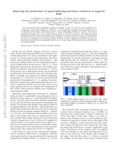
DESCRIPTION OF THE INSTRUMENT Figure 1 is a schematic showing the position of the single loop sense coils relative to the sample access, which in this instrument has a diameter of 6.8cm. The coils and sensors are surrounded by a superconducting lead shield which has the capability of "freezing in" the field in which it is allowed to cool below the shield transition temperature. It is clear from Figure 1 that only the vertical axis coil is of the true Helmholtz design, the two horizontal coils having a rectangular shape which in turn is curved around the dewar wall. Additional shielding is used above and below the detector coils to ensure the sample moment only couples with the coils within a limited region. In this way a zero reading can be taken with the sample only a small distance away from the detection region. The outputs of each coil sensor are calibrated by the manufacturers who use a small solenoid whose equivalent moment is known. Since each coil measures the total (remanent plus induced) moment, along each axis, it is necessary to make remanent moment measurements in a low field. How large a field can he tolerated depends on the magnetic characteristics of the samples being measured. In practice, a field smaller than 20 nT is usually found to be satisfactory. In this study, the maximum magnetic field within the detection region was less than 10 nT. The field gradients were less than 1 nT/cm (1 nT = 10 -5 gauss = 1 gamma).
2
RESPONSE OF THE DETECTOR COILS
The spatial variation of the output of each of the three axes was checked using a small (lmm diameter) sample, which was given a saturation moment along one of its axes. Profiles of output versus vertical position were then obtained for each of the twelve horizontal positions shown in Figure 2. These profiles are shown in Figure 3• The sample was oriented so that its moment was along the axis being tested in each case. The figures adjacent to each profile represent, the value of the output (ir. arbitrary units) at the mid point of each profile. The results indicate that the region within which the response is uniform to within a few percent is fairly limited. The vertical axis defines the minimum volume of uniform response, which is a cylinder approximately 4 cm long and 2.5 cm in diameter, within which the variation in output is less than 5%. The horizontal axes responses are similarly uniform within a larger volume - a cylinder about 6 cm long and 3 cm in diameter. Although these volumes include the standard 2.5 cm diameter cores used in most paleomagnetic studies, it must be emphasized that these results are for a 6.8 cm access instrument. For the more common 3.8 cm access instrument,the volume of uniform response would be correspondingly smaller,and almost certainly less than the standard core volume. The amount of error that this would cause in a single measurement would depend on the degree of inhomogeneity in the sample being measured. However, it is clear that significant errors could be introduced in this fashion.
3
I
CALIBRATION PROCEDURES: Absolute Calibrations were made using a small (0.476 cm diameter) 5 turn coil. The equivalent dipole moment of this coil was taken as M = nIA/10 emu where A is the area of the coil in cm2 , n is the number of turns and I 4S the current in amperes. The coil was positioned at the mid -point of the vertical response profile shown in Figure 3 (Z) and the current varied by an amount -4 corresponding to 10 emu (1.12 mA). The calibration potentiometers in the magnetometer electronics were then adjusted tn give corresponding -4 changes in the magnetometer readouts of 10 emu,with the coil oriented along each axis in turn. The calibrations agreed to within a few percent with those performed by the manufacturers with the exception of the X sensor,which had recently been replaced and not subsequently recalibrated. Goree and Fuller (1976) have reported significant non-linearities in the output of their instrument. Linearity was therefore checked on the x10 range by plotting magnetometer output versus coil current, a with the coil. The results indicated that linearity was better than 0.5% for all three axes. The experiment was also repeated for the X100 range with similar results.
4
^ r
AXIS ORIENTATIONS The effective orientation of each axis was checked using a sample with most of its moment directed along a single axis. The direction of the major moment was then positioned at ten degree intervals in a plane at right angles to the axis being tested. In this way, cross-coupling effects show up as a variation in the output of the axis being tested, which should remain constant if the axes are truly orthogonal. The results are shown in Figure 4 (a), (b), and (c). They indicate small amounts (about 1%) of cross coupling between all three axes. Since the variations are approximately sinusoidal, it should be possible to correct for these effects using cross coupling coefficients whose values are known. If the true values of the three orthogonal components in the sample are X, Y, Z and the observed values X l , Y 1 , Z 1 , then X 1 = X + CyxY + CzXZ
(1)
Y 1 = Y + C xy X + C zy Z
(2)
Z1 = Z i C xz X + CyzZ
(3)
The cross-coupling terms C, xy , C Xz ... can be estimated from the plots in Figure 4. However, a more convenient way to estimate them is to measure a calibration sample in different orientations. The calculations are considerably simplified if the calibration sample has most of its moment along one axis,as each cross-coupling term can then be estimated independently. Two measurements are then required for each cross coupling term. For example, to obtain C yx , the major moment of the sample is oriented along the Y axis, and the value
I 5
^ V
X 1 measured. The Y and Z components are then inverted by rotating the sample 180 0 about its X axis and a second value of X 1 obtained.
It then follows 4rom equation (1) that the difference between the first and second values of X 1 will be 2C yx Y, provided the last term,
C Zx Z, is assumed negligible in both instances. If Y 1 is assumed equal to Y, the coefficient Cyx can then be obtained. A more complete determination of the coefficients can be made using appropriate measurements on any sample at all. However, this will clearly involve inversion of a matrix which the above method avoids. Shown in Table 1 are the results of measurements of a calibration
sample with its cubical sample holder oriented in all possible (24) positions relative to the magnetometer measuring axes. This data can be used to obtain four independent estimates of each cross coupling term by suitably combining the data in the manner already described.
The average values of the cross-coupling terms so obtained also appear in Table 1. The additional terms Cxx , Cyy , and C Zz are calibration normalisation terms. These were calculated by averaging
all the measurements of the main component of magnetization for each axis, then normalising the results to the average value for the Z axis. In this way, calibration errors between the three axes
are corrected for. The results of applying the corrections according to equations ( 1), (2), and ( 3) appear in Table 2. It is apparent
that the scatter in the results has been reduced from almost 2 0 to less than 0.20 . Tables 3 and 4 show the results of similar measurements on a 2.5 cm diameter core of fine-grained basalt. Again, a considerable reduction in the scatter of the results is evident.
6
I
_ J
This reduction in scatter can be more easily seen in Figure b, which shows plots of inclination versus declination before and after correction for cross-coupling for the basalt sample. The slightly larger scatter of the corrected results in Table 4 (about 0.5 0 ) is probably due to
the larger size of this sample compared to the original calibration sample, whi0 was only — 2 mm in diameter and 2 mm in length. The directional variation may therefore be due to small inhomogeneities in the rock sample causing differences in the coil responses as outlined in the previous section. One interesting feature of the cross coupling coefficients shown in Table 1 is that, for example, C xy is not the same as Cyx .
This
implies that the coupling cannot simply be attributed to misalignment of the coils, for this would clearly imply that these two terms should be equal. Some of the coupling is probably between the wires leading up to each coil and the other coils. This would explain the no-icommutative behavior of the coupling terms.
I
7
NOISE MEASUREMENTS Shown in Figure 5 are output traces recorded over a 5 minute period using the lhz bandwidth filter. The traces also show deflections recorded for insertion of samples having the indicated moments. The short term noise varies from about 2x10 -8 emu r.m.s. for the x axis to 1x10 8 emu r.m.s. for the Z axis. The lon g term drift ran ges from 5x10⁻⁹ emu/min for the Z axis to 2x10 -8 emu/min for the Y axis. The larger drift in the horizontal sensor outputs seemed to be related to less effective shielding in the horizontal directions. It was found experimentally that a magnet producing 10 gauss at the sense coils caused a change of 10 -5 emu in the outputs of the horizontal sensors. This implied that field changes of 0.01 gauss, which are fairly common in urban evnironments* can cause observable noise in these magnetometers outputs. The vertical shielding factor is much greater - the 10 gauss magnet produced no observable change in the output of the vertical sensor.
8
V
.M
DISCUSSION Superconducting magnetometers of this type are clearly useful instruments for measuring weak magnetization in paleomagnetic samples. Although their spatial response characteristics are clearly more uniform than those of either spinner magnetometer coils or fluxgates, significant variations are nevertheless present. To eliminate the effect of these, measurements need to be performed with samples in different orientations and the results averaged as has been done with spinner magnetometer data. It has been shown that with suitable precautions, a ore-inch diameter core can be measured with a single insertion to an angular accuracy of better than 0.5 0 . However, with a 3.8 cm access instrument, the angular
error could be much greater.
9
REFERENCES Goree, W. S. and Fuller, M., "Magnetometers using RF driven SQUIDS and their applications in rock magnetism and paleomagnetism" Rev. Geophys. Sp. Phys. v. 14, No. 4, pp. 591-608, 1976.
10
s
TABLES
Table 1 - Measurements of _ alibration sample in different orientations. Also shown are the cross coupling terms calculated from this set of measurements using the methods described in the text. Table 2 - Corrected calibration sample measurements. Note the large reduction in scatter compared to Table 1. Table 3 - Measurements similar to those in Table 1, for a 2.5 cm diameter core of fine grained basalt. Table 4 - Corrected results for the basalt core.
FIGURE CAPTIONS Figure 1 - Sense coil geometry for a two-axis system. Figure 2 - Horizontal positions of response profiles. The numbers in the circles correspond to the numbers on the left hand side of each of the profiles in Figure 3. Figure 3 - Response of each axis to a sample as a function of vertical position in each of the positions defined in Figure 2. The numbers at the center of each profile are the output moment values (arbitrary units) at the optimum position defined by the vertical responses. (See text) Figure 4 - Cross coupling response for: (a) the X axis, (b) the Y axis and (c) the Z axis. The upper two curves in each case are the variations in output of two of the axes when the sample is rotated about the third axis. The lower curve is the variation in the response of this third axis, which for no cross coupling, should be zero. Figure 5 - Noise measurements made over 5 to 7 minute periods (not synchronously) for each axis. Also shown is the effect of inserting the small moments indicated, into the sense region. Figure 6 - Plots of inclination, versus declination for the basalt core as measured in all 24 orientations, before and after correction for cross-coupling effects.
:~
14
O 41
O
O
a
O +
J Cl 0 4 41 ^
00wr1Nr-40m
t^000OlOOM
C;C O4 0
f! Od^l+01 0
N
ae
..
I,0A 4J
c3
q
m
H co
Of
m ^
O
14 O
1
+-) O
Ata
1
r1000^i'd^0! OO qOC 0 C C;
^
0>V4
^d
0w
as
O
m a 0
rIrIrIrIrIMmrImmrIrIrIrIH rIriri e-4r4r4ri1-4r1
0 0 0 0 0 0 0 0 0 0 0 O O O O O O O O O O O O O
^+
rI
0
00 t` On t- 00 00 00 OD 00 00 t- h 00 t- 00 t- 00 00 00 00 00 00 t- tc+'1 M M M M M M M M M M M m M M M C V) M M M M M M M
1
^ 0)
a 4-)
0NNt ,-vwtoMv0)r-4Nt^-0wm(D 0 Cq 0 mto0 r100"400rINMMM C V) a000NODr-1 t- r4r404NN. -4 t- t-
IV
q
+)
gg5'qq4`?qqqqqqqqqqqqqqqqq wwagwpllgwwwwrqlqwNwlqwwwwwwaalq
Q
rl
1
E
N
O i^
Iv CI W
rI000gOr10a
.0
w
w >C
A
^
13
M to O t0 h O t^ ti to N O 01 cA N N N 00 rA eM M^^ t0 O
A
(AOOOrII^I^rII^MI^[^tOr-^Q^Or10Cflrf00riCOt^l^ t0 t0 t0 t` ti t0 00 t0 CO N N t0 t: t0 t0 t^ t: t0 00 t0 tO t: t: t0 OD 00 00 00 00 00 00 W 00 OO 00 00 00 00 M OO W W OO OO 00 M 00 M
0)
aY
00 00 00 00 00 00 00 00 00 00 00 00 00000 00 00 00 00 00 00 0O 0O 0O tiOd^0000d^Nt0ON C0 t` NO rir-I ON ri Ot^d^'d^
N Ot^Ol^d^rtCOrlptA00t^M000fl[^CONrIrlOtf)l`t0 p
M
p
MrINON O ^MOMq^r; N
i
I
O
i'
1
q
t: e)m
1
tr• O
OD O O O O O O r1
ri
h
p
O O O O O O O O O O O O O O O O O O O O O O O O ^ ^ t OO ti N 000 ^ 000 C00 ^ O ^ O M ^ C00 « ^ M 000 ^ N ^ ^ M ^+ OOOOOMNMNNMd ^MC^0000N V r Hr-frINM p p NNNri ) I1 O MMMM 1 O I I NN C;MMce)m
1 I 1 1
000000000000000000000000
000000000000000000000000
N eM t• O d^ O0 r+ r-i M 00 N 00 t` d' M l^ O O d' [^ N ^ ti N yC r+ 000 rI rI NOd^N Or-IritOe -ItOrIriNM ►f^Oerrl
M O MI
O
gM0 r O MM 1 rIN 0 ;INMM 1
1
C grlN
n
'r4 > N N N N U U U
as
fa
A rl
cis
U w 0 In
C O CO r! O
. O
t- v t- t00 O m O
C; O O
41
0 O
rn
cO
n
n
a
U
U
U
(D
x
1
er M N p 00 Q^ O O
m O O C; q It
11 x
U
it
K U U^
O ri
A
cO E
O
•^ O
O
r-I r-I
r-I
Ir
1= t0
0) •^
ra r-i H rl r-1 ri i-I r-I r-I ri r•1 rl rl ri r♦ r-1 r-I r i r-I H -4 r-I r-1
g 4 q, gq 444444 qq 4444 qq 444° q 0 0 000 000 000 00Otiti00Oti NNt- to - 00 000 00 0 00 ti00 0 00 0t 0 0 0 00 ti^tiNNti[^NtiNNN[^Nt`h^t` tiN[^[^N[^• m CO) m MMt+9MMMMMc+9MMMm ce)mMMMMMM O O O O O O O O O O O O O O O O O O O O O O O O wwwwwwwwwwwwwwwwwwwwwwww
_
In
w
;4
r4
:1 ^ O
•rI
:3
s~ O
0
+^ d
O
O x Q
0> -H iJ
bO Q
0^
Cd ca
1
i
r•I
o) a)
o
Q ;4
E-4
O
^
k
y
1
I
(1)
r-I w
I~ ou
02
^„^
tc^ pp Md^000000MO1^r-Ir-I^t'3tDN[^N d^C ^. tn(^O u7 d^ u^ d^d 'trMMd+d^OCfl^d^d^d^ (o cAtA epe MMeMd^ e e e e o e e • e • e s s e
•
o
o
o
•
o
•
a
1^i
Q
•R
r.
O
o
O O O O O O O O O O O O O O O O O O O O O O O O li
Q
c0 v m m w m O d' M I^ M r-I OO h O O GO M ^[i N N O ^l M r • I MNNN 000 r-1 0 r - 1r-I Nri 1-I NN OO 000NNN o • • • e e e • • 0 e e • 0 0 • 0 e e 0 0 D . OtiLOht`t`+ >•,
>>
U U U • M t` d + ri N d+ O O d' t` O M M O 0! O O h h O0 rI ^t ! p CO M O t^ N [^ l^ r-I r-^ CO CD O ^A O r-I mv0TN0m00Nvt-v00r-I0t-061000r-I [^M[rM1^000OMt^MO00Dt^M00Mt^t^0ON00Mt^00 . o • . 0 0 0 0 0 e 0 0 e O e D . . 0 0 0 0 0 0 p p p 1 rl I M 0 M 1 Cj M 'H O r^l s^ r•^ ri M O M 1mm 1 p C1 00 0 M to r I ri
-
'^'
I
..O 0) ^V C
(
O
U N >D
N W
H
1
1
1
.Q tK
E-+
M
v
p
^ a^ D
I
00
o
a
O
I
'
N
"1
>G 5C
O.
°
4
I
II >+ >C
U U U
AO
N x
^,
_Aj
N N N N N N N N N N N N N N N N N N N N N N N N g 4 gqqq 4 q 4444 qq 444 q 4444 q 4
•
4J
wwwwwwwwwwwwwwwwwwwwwwww
^
:q t^MC^lCMlOoC^OCf00t^r^IMcD^0^NOp00r^-IOpNMMpMN dt el' dt M ef' d t O dl dt elt v v o o O to d t e11 O O to O O
co
O^C^C^C^O^CAd^4^00^0A0AC^0^0^C^CfO^C^O^OA OAC^d!
N A
O O O O O O O O O O O 0 0 0 0 0 0 0 0 0 0 0 0 0 A
14 o m o vCflr I--I
o
•
CldtOltt> IM C^Nd^N^^^OeN^Oid^G^ON ^Mt^C • • e o • • • e • • e s w • e e • • e •
C; 0;
0; C; d d^^ dC^d^C C; r 4
dd
N r-I NNNNNNr-1NNNNNNr-INNNNNNNN
be
O
O
w w
O
A
r4 t-t-00t-d e l-WVMH MWN 0 t-mf-40McflNLOcfl Lr) w.• v 00omo(7)•• C4 04 00 m 0 t- C 14 CD m0 r-I t-MGot-0 e o o e • o e• o s •••• ••• s to v14OmtovOtnL t dt^tOOOOdteM 4L4V OOOMOOOOOOOOOOOOOtnOOO to LO r-I rI r^I ri r-i H H r-I r-I r-I r-I r-I r-I r-I r-I r-I r-I ri r1 r-1 H r-I r-I r-I
O0 O0 O0 O0 O0 O0 O0 OQp OO OO OO OO Opp O0 O0 O0 O0 O0 O0 O0 O0 O0 O0 O0 OMOCp N^00 tt^MNNCp1!'1 rlOO p Op COMOOONO
41 ;4 O U U O I N
O
N M00MnO0MONO Cfl [^draOM 00 0CAMO ^t OOQ^ 0 0 o e e • e • • • s ♦ o e o • . s e • • o e • MMMMOOt^M00M00MMMMMM001^M00M00MM
O ^ +^
OO OO OO Opp O O O O O O O O O O O O O O O O O O O O O O O O O O O O O O O O O O O O O O O WN00 to Oa0dt OM0000d + N Od'NO OtD CflriCO
co
1 1
I
1 1
1
I I
1
i l l
s~ O 1~ s♦O ^
D+ O O m m N M t- t- t- t- "I N r1 O O rl M v t- w t- t- M M
0000 t: t-o MO t+9MMMme M, me wo W, W* wo MM* M* M* +M MO mo M
I I I I I
I
I
I I 1 1 1
0 0 0 0 0 0 0 0 0 0 0 0 0 0 0 0 0 0 0 0 0 0 0 0 9C
t-tD000CD0to mCO'IC0C CD NF-4Innpr01000(3)ttM 0)LOCN CflrI00MtCC^raMON000C 1nONt^I^OMO^r •-10 M M tM M m M 00 M OF M I I 1
00
00 tM M Mm M M 00 M I I I I I
00
M 00 00 I I I
'C 0) U Q) fti V `a M O ri
A
al
E
N N N N N N N N N N N N N N N N N N N N N N N N
gg4qqq44q44q4qq4444qqqq4 wwwwwwwwwwwwwwwwwwwwwwwaa hV^eNd^l^r-IC^I^[^C1^o0eMM000^MU^N ^cIMODCf
•-I toMt-000v v 000"0DMM oN00MC mmm d^ M M N M d t d t LA 'd^ M e!^ M eN d^ dt d^ eM d t M to dt ^ M d^ Q^ O O O Qs Qs Of O
Q1
D! 01 01
Qs
01 0! 0 07 O 0 Q1 O eA 01 D!
0 0 0 0 0 0 0 0 0 0 0 0 0 0 0 0 0 0 0 0 0 0 0 0 M
ON OcC^-INOd^OtOl^Od^CC^^Nd^M00^OMt^d^
0
N N N ra ON O N NO NONON ON O N O N NONON0N0N0N0 N0 N0 N0 N0 0 N
rQ L^
O CD r-I C1 M Q^ N d^ O O r1 M N M tD to N h N
r-1
O r`I
Lo t`
CD d^ dt
Q1
E to
OOP-4r4 r-I N t^P-ONt^000N ^AN^-IOOtCI^GO^eNONMQ^OCO
ca d rel
LO Lo Lo M kf) r-I r4 r-4 r-I r-4
to to r •t H
LO to LM to to to 1"
M
to
r"I
1" I P4 r`I H
4
H
to O M
to to to LO Lo to r`1 ri r-I r-I i" I r-f r-I r'4 ra H
^Md^00^r-IOOr-INPiM^OI^OIMOMO^L^C^OM t`^N M O ei' r-I P'1 to Lo 00 O M M 01 00 t7^ O p 00 CD M d^ .-1 to CD O e-1 O Op ^ O O O ^ ,^ LA N tG O ^ O l^ N CO [^ r^ 0^ O c0 0! r-1 O N Mt^Mt-M0)V 0MCDt-t-Mt-Mt-00NP-1MMt-00 o
•
•
.
.
.
.
.
.
.
.
.
o
.
•
1
1
•
•
e
M M M M N N M OD M ti M M M M M M 00 OQ M 00 M [^ M M I
'^.,
I
1
I
11
1
L
1
1
1
^'NCA^+ ONr'tOCDCDd^eMd^0000NCflMOMOM00r^ O d 1 OD 00 N M t` t` CD CD N N O C1 O O N M t` ti t- t- N M
t: t` tz t: M M M M M M M M 00 t: t-* O0 M M fM M4 C M cM M
i
I
I
I
I
I
1
1
1
1
RI
to fy
O
W
W
l^r-^r-I tt^d+ NONMQ1CfMMMeNOOd^Mt^d + r-t 00 r-1 C's eM M O 0 00 r1 M N eM e-1 M rl N O 00 O 00 00 MOM CD t1) I
to
1
r^l O to tU .O
O C) O fi
O
^C
r-4 0OwvMOo r-1 " M r4 NCNN ra vto N"rimOO ww00t-Ov t- Ot- ON t-v"00MwN0 vvcv) v m t- (D v CY) 00 0 " tD 0 14 " P-4 wNt-tDCDMCflN00M
t^NCD 44r t.OM 0m0mt^Mt^cnw CDmm0m 0 0 M M M M M M t- M i M 00 t` M M M M M M t` M OO M ti 00 1
1
1
I
1
1
1
1
1
1
1
v d^ O r-1
Ac0 E
Sensor Output ------
Superconducting Sensor
CEED Field Tronsfer Coil
elmholtz eometry ickup Coils
Fig. I SENSE COIL GEOMETRY (TWO-AXIS SYSTEM)
r
I
xcm oo,^
E 0 co
0
o
a
o q
r
i__
► to
X5
C4 OD LLB
Y Awl&
1 2 3 4 s 6 T 6 9 10 12
1 2 3 4 5 6 7 e 9 10 it 12
DISTANCE FROM BOTTOM OF MAGNETOMETER ACCESS(CM)
Fig. 3
1
^
^^
ZRRS
sx
^^^^
74
Q q 'R
N
- M g e ^t
v
00
^
I
R• R R s s 3^;^
Iw..a .1
d!
Z
I
A
O r O
b
0
x es !V
0 r 1
un oc
w
N!
N
h
y
x
0
w_
0 cD
LO
•
Z
O
H
••
w
in a ~
••
• •
O V
LO 2
U
• •• ••
cr
1
•
O
•
00
00
v
.o w
• •• W W ^ L •
• Z O o
••
r) Q LO Z_
• •
J
U
W
V ZD
0
• •
v
• t
v
N
o O
N
NOIIVNI-lZ)NI
0 Q^