the system is able to dynamically adapt itself to input data and external events. For example ... adapt itself to the external events that happen in the scene can outperform the ... acquisition or processing for recovery of degraded images. Atmospheric ..... Based Readback Signal Generator For Hard-Drive Read. Channel ...
Improving Performance and Quality thru Hardware Reconfiguration: Potentials and Adaptive Object Tracking Case Study Soheil Ghiasi, Hyun J. Moon, Majid Sarrafzadeh Computer Science Department University of California, Los Angeles {soheil, hjmoon, majid}@cs.ucla.edu Abstract Reconfigurable hardware devices are envisioned as the proper platform to implement multimedia applications, providing both real time performance and dynamic adaptability for the application. In this paper, we discuss the issues involved in using reconfigurable hardware devices for multimedia applications. The ideas and approach are then applied to a collaborative object tracking system that has been built as part of our work. We justify the need for dynamic adaptation of the system through examples. Experimental results on a set of scenes advocate the fact that our dynamically adaptive system works effectively for different scenes and scenario of events, and it outperforms traditional pure software or hardware implementations.
1. Introduction Many multimedia applications perform intensive computations, yet they have to cope with severe performance constraints. Pure software implementations of these applications on constrained embedded processors do not exhibit satisfactory performance. Therefore, such applications demand hardware implementation to exhibit real-time performance. Dedicated hardware solutions exploit the intrinsic parallelism of multimedia applications and execute many operations in parallel, which leads to substantial improvements in application runtime. Many researchers have used hardware implementations to speed up the application runtime [1, 2, 10, 16]. Another characteristic of multimedia applications is their sensitivity to input data stream. Usually, there are several different methods to process the input data, while each method is effective/optimized for a particular input data pattern. Therefore, the application’s quality can be greatly enhanced if the system is able to dynamically adapt itself to input data and external events. For example, tracking an object is a basic vision functionality that is utilized by many high-level applications such as traffic control and intruder monitoring systems. Commonly used trackers employ a number of vision algorithms for tracking a moving object. Each algorithm can be parameterized/is designed to perform with higher quality for a particular working condition such as a particular lighting condition, object shape, distance or resolution. Therefore, a tracking system that can dynamically adapt itself to the external events that happen in the scene can
outperform the corresponding static implementation in terms of tracking quality [8]. While dedicated hardware implementations successfully tackle the problem of real time performance constraint, they are not flexible enough to address the dynamic adaptability issue of the system. Traditional hardware implementations are not alterable at runtime and therefore, the application’s quality cannot be improved by exploiting a particular characteristic of the input data. The aforementioned arguments introduce the reconfigurable fabrics as an efficient solution for implementing multimedia applications. Reconfigurable hardware units not only demonstrate real time performance by exploiting the intrinsic parallelism of multimedia applications, but they also provide the required dynamic flexibility and adaptability for the system. Both of these objectives cannot be achieved by traditional pure software or hardware implementations on constrained embedded processors. Reconfigurable hardware devices are often coupled with a general-purpose processor that controls its parameterizations and reconfigurations [3]. Efficient partitioning of a given application onto a reconfigurable fabric and its coupled processor has been subject to extensive research in the past and present. Currently, there is no widely accepted methodology for implementing an arbitrary application on such a platform. Therefore, an effective automated approach that is applicable to many multimedia applications is of great importance. However, before presenting such a general methodology, we focus on a case study (a collaborative object tracking system) to motivate the need for dynamic adaptability and verify its performance and quality improvements over a pure software and hardware implementation respectively. We proceed to describe two image-processing algorithms that are used in many tracking-based multimedia applications, namely feature selection and image restoration, in Section 2. In addition, the effect of external events and environmental changes on these algorithms and hence, the need for system adaptability are explained in that section. Section 3 presents our experimental platform, which is the used to verify the ideas and approach presented in this paper. Section 4 discusses the challenges involved in implementation of the tracking algorithms. Section 5 presents the experimental results that verify the effectiveness of the dynamic adaptable system in practice. Finally, section 6 outlines the conclusions and some future directions.
2. Vision Algorithms and Their Sensitivity to Input Data In this section, we present two algorithms that are required for enhancing the image quality and tracking the motions, i.e., image restoration and feature selection. First, we outline the algorithms’ underlying idea and functionality. Then, we describe their sensitivity to the changes in the scene.
2.1 Feature Selection KLT tracking scheme [5, 6, 7], which is widely used in object tracking applications, is carried out in two stages. In the first stage, called feature selection, proper points in the images are selected. These points are passed on to the second stage, called feature tracking, in order to find their location in the consequent images. Feature selection algorithm consists of carefully choosing the points in the image, which can be easily tracked throughout a series of images. Corner points of an object, where intensity changes noticeably, are considered as good feature points with good trackablity. The feature selection algorithm computes a complex function, F, for each pixel and compares its result with a fixed threshold value, λ. Function F assumes a square window around each pixel and performs its computations using the intensity values of pixels inside the window. If the value of F for a pixel is larger than λ, that pixel is declared as a feature point; otherwise, it is not a feature point. Function F solely depends on the intensity of the pixels inside the window and does not change with time or other parameters. Therefore, the number of selected features reduces with the increase of λ and vice versa. Hence, points that are selected with higher values of λ are considered as better features. Note that such features are also selected with small values of λ. These points are usually easier to track in consequent images. They exhibit significant intensity variation compared to their neighboring pixels. Figure 1 demonstrates the output of the feature selection on a selected region of a sample image. The feature tracking stage of the KLT tracking method strives to locate the selected features in the next frame. This is performed with the assumption that the two consecutive images differ only by a small displacement factor. The tracked features will be tracked again in the future upcoming frames. Therefore, the displacement, motion direction, velocity and other information about the motion can be inferred. The latency of feature tracking stage is directly proportional to the number of selected features and hence, a large number of features makes tracking to slow down. On the other hand, a small number of features is not sufficient for high quality tracking, since tracking might ‘lose’ some features as the object moves. Therefore, the number of selected features should be within a specific range in order to maintain a balanced trade off between tracking quality and performance. However, many changes in the scene such as lighting or distance variations alter the intensity of the pixels. Therefore, a fixedimplementation of feature selection algorithm cannot control the number of selected features. This issue can be handled by software implementation, however feature selection software realizations run quite slow on most of constrained embedded processors. Reconfigurable hardware devices seem to be the only proper platform for implementing this (and similar) algorithm (s) for multimedia applications.
Figure 1. Feature selection algorithm performed on a sample image. Selected features are denoted by small dark squares.
2.2 Image Restoration Image restoration is a commonly used algorithm in image acquisition or processing for recovery of degraded images. Atmospheric turbulence, defocusing or motion of objects can be reasons of degradation. Restoration process recovers lost information of images by such degradation [13, 17, ]. The following degradation model holds in a large number of applications [13]:
y (i, j ) = d (i, j ) * *x(i, j )
where x(i, j) and y(i, j) denote the original and observed degraded image respectively. d(i, j) represents the impulse response of the degradation system, and ** stands for twodimensional (2D) discrete linear convolution. The goal of image restoration is to estimate x(i, j) given y(i, j) and d(i, j), however one of the main difficulties in performing an ideal image restoration is that the degradation model is not completely known. In other words, d(i, j) is not exactly defined/known at the receiver. Therefore, it might not be able to completely reconstruct the image. Image restoration is often implemented as a filter that is applied onto captured images. Noise signal injected into the image usually exhibits quick variations and hence, is considered high frequency signal. Therefore, common realizations of noiseremoval filters implement a low-pass filter, which allows the image signal to pass and filters out the high-frequency noise. A low-pass filter has no effect on low frequency image data (pixels with small variations compared to neighboring pixels) and removes the high frequency elements of the signal. As a result, the sharp edges of an image passed through a low-pass filter become blurred while the solid textures remain intact. On the other hand, blurred and defocused images have to be passed through a high pass filter in order to be restored. The high pass filter restores such images by sharpening and/or preserving their edges. Therefore, based on the captured image deficiency (noise or unfocused lens and blurred edges) different filters should be applied to restore the image. Dynamically adaptable implementations of the filters should be able to enable/disable the filter or alter its coefficients at runtime.
3. Case Study: Adaptive Object Tracking System In this section, we present a collaborative object tracking system that has been implemented in our lab [11]. The idea of dynamic system adaptation to external events is practiced in this system as a case study. The advantages of this approach and comparisons with non-adaptive systems are presented in experimental result section. The framework for our system is comprised of two IQeye3 cameras provided by IQinVision [4], pan-tilt units to enable the actuation of the cameras, a main controller residing on a PC, and a network for communication. An IQeye3 camera, as a “smart” vision sensor, with embedded computation resources allows input image data acquisition and processing to be collocated in the camera, which minimizes network communication overhead and facilitates scalability. The processing resources embedded in each camera include a Xilinx Virtex 1000E FPGA [15] and a 250 MIPS PowerPC CPU (Figure 2). In addition, there is 4 MB of Flash RAM and 16 MB of SDRAM on each camera. The embedded FPGA is utilized for implementation of intensive image processing algorithms, while a simple controlling software code executes on the embedded processor that controls the reconfiguration and parameterization of the FPGA. Figure 2 demonstrates our system with two cameras and the main controller. The main supervisory controller resides on a PC and acts as the centralized governing unit of the system by maintaining the current state, processing internal and external triggers, and coordinating the collaboration among the cameras. When the main controller receives data from one of the IQeye3 camera clients over the network, it deterministically selects the appropriate actions that should be taken by each camera (e.g., reconfiguring an embedded FPGA by swapping in a different algorithm from the database (Figure 2)). This is performed by sending a message to the designated camera. The sample application implemented on the framework is to continuously detect and track a moving object that is within the field of view of a camera. We assume that the object is always moving across the camera and hence, KLT tracking scheme [5, 6, 7] can effectively track the motions. When the entire system initializes, cameras establish a connection with the main supervisory controller on the PC.
Camera 1 assumes control initially and continuously runs feature selection algorithm on its embedded FPGA. As the objects in the scene, distance of the object to the camera, light conditions, lens focus and other parameters change the number of selected features varies. For example, two runs of the algorithm on two different objects will lead to selecting a smaller number of features for the object with fewer corners and intensity variations. Our implementation can detect such conditions and can adapt itself in order to compensate the effect of external parameters to select constant number of features. Therefore, it is ensured that the number of selected features, and hence both latency and tracking accuracy, are kept within a certain range. This is accomplished through reconfiguration and parameterization of the algorithms running on the embedded FPGA. Furthermore, when a moving object moves close to the edge of the field of view, the camera can no longer track the object. In this situation, the camera notifies the main controller by sending a message indicating the position where the moving object is located. The main controller then decides which camera should gain control and sends an appropriate camera a message indicating where the object is. Figure 2 outlines the architecture and application of the system. A sample pseudo code running on the controller and a high-level block diagram of each camera have been demonstrated. Note that each camera has a database of required algorithms locally available.
4. Hardware Implementations In this section, we describe our system constraints and the modifications we had to make to the original algorithms in order fit them to our platform. Moreover, we discuss the system adaptability issue in our implementations.
4.1 Platform Constraints IQeye3 camera is the vision sensor used in our platform. The camera imager continuously captures scenes and injects a non flow-controllable real-time stream of image pixels into FPGA at 24 MHz. FPGA then performs several operations on the stream such as image correction, windowing and down sampling. Then, a DMA unit residing on the FPGA stores the processed Controller
Initiate algorithm Y
Initiate algorithm X Scene Data
FPGA Processor
Algorithm Database
Computation results
Motion Detection Feature Selection Image Restoration
I/O controller
Camera 2
Camera 1 Moving object
Figure 2. Dynamic adaptation of the system. Each camera has access to a database of algorithms. The controller initiates the reconfiguration to realize the proper algorithm. It also maintains the coordination among cameras.
scene data in the main memory. The FPGA is clocked at 33 MHz. Any program running on the PowerPC can access the memory and the image data stored there. Within this environment and platform, image-processing applications sitting on the FPGA need to meet some constraints. The most important issue is the timing constraint of the design, since the imager stream is not flow-controllable. Therefore, the applications have to process the input stream and generate the corresponding output at the same rate to avoid congestion. This forces many designs to perform their intended computations with the small on-chip memory, because using off-chip memory unit will impose additional latency, which is not tolerable for many designs. Furthermore, there is a system design continuously running on the FPGA. This design performs basic necessary image manipulation functions such as windowing and packetizing. Any application mapped onto the FPGA has to integrate with this design and has to cope with its communication standards and data formats. Therefore, the algorithms cannot be used in their original form and have to be adapted to our constrained platform.
4.2 Implementations As mentioned in the previous section, the main challenge for implementing the algorithms on the camera FPGA is that there is not enough on-chip memory available to store the entire image. Moreover, tight performance constraints do not allow us to use an off-chip memory module. Therefore, we had to modify the algorithms such that they could perform their intended computations with limited amount of memory. The stream of image data injects pixels starting from the upperleft corner to the right. After streaming each row, a control pixel is injected and then the next row is streamed in. Figure 3 demonstrates the idea of our hardware implementations. For each pixel, we store slightly more than two rows of the image, in order to maintain a 3x3 window around that pixel on the chip. Therefore, we can perform many computations with the window pixels within the delay constraint. Note that, the amount of required on-chip memory grows linearly with the size of window (assuming that the window size is too small compared to the image size). Hence, larger window sizes or dynamically variable window sizes can be implemented on large enough FPGAs.
n nn • ncn • n nn
• • • •
height
• • • • • •
Processing window (3×3)
width Figure 3. Image frame and processing window. c is the center pixel on which the computation is carried and n’s represent the neighbor pixels. In this example, two rows of the image frame need to be stored on-chip.
The feature selection algorithm performs computations using only pixels in the 3x3 window around a pixel to determine whether it is a feature or not. This algorithm has been implemented on the same platform in a previous work [9, 14] using this method. The result of the computations is compared with a fixed threshold to determine the features. While this implementation works well in practice, it does not have any control on the number of selected features. Moreover, the value of threshold cannot be altered easily, because threshold has been implemented as a constant, which must be specified at design time. Various parameters such as objects’ shape, scene light and lens focus can affect the number of selected features. As mentioned before, the selected features are passed to the tracking phase. The latency of the tracking grows, while its accuracy drops, with the increase number of selected features. Therefore, the number of selected features has to be controlled in order to maintain a proper tradeoff between the latency of tracking and its accuracy. Our implementation is similar to [14], however we have modified the original design such that the threshold value can be dynamically controlled by a program running on camera PowerPC. This was not a trivial modification of the basic design, since there is a system design continuously running on the FPGA. This design performs basic image processing routines such as image quality enhancement, packetizing, and transferring the final output to the system memory through DMA. Every modification to the system has to cope with this basic design and has to adopt its communication standards and data formats. Software-controlled threshold value, has enabled the dynamic adaptation feature of the feature selection algorithm. According to the algorithm, if the threshold used in feature selection is too low for a particular scene, we get too many features and if the threshold is too high, we get too few features. Therefore, given a target number of features desired, we increase the threshold if we get features more than the target and decrease if we get less. Note that the feature selection algorithm performs its computations on the FPGA and exhibits real time performance. The threshold controlling entity is a small program running on the camera PowerPC, which counts the number of selected features and controls the threshold value accordingly. On the other hand, image restoration has a variety of implementation and iterative method is a widely used one. The purpose is to estimate the original image given the degraded image. The original implementation performs operations on the entire image iteratively. The iteration is stopped when the restored image converges with insignificant residual ε [13]. We have made several modifications to adapt the original method to our environment. Instead of globally iterating over the entire image, we iterate over local windows, where the size of window can be from 3x3 to the entire image. Researchers in [13] have shown that the algorithm implemented as described above, has reasonable restoration quality. As the window gets smaller, the restoration quality drops since the center pixel (Figure 3) does not have any information about pixels out of the restoration window. However, this enables processing of image stream using a small-sized storage. Moreover, we showed that iteration over a small window could be unrolled a priori. Therefore, iterative image restoration can be replaced by a simple non-iterative process that performs the very same algorithm using less hardware resources. Particularly, we have gained 11% improvement in terms of the number of utilized CLBs on a Virtex1000E FPGA chip. This percentage is
more significant for smaller devices that have a smaller number of CLBs. Varying the restoration window size leads to accuracy-memory requirement tradeoff. Small restoration windows need smaller on-chip storage, however their quality is not as good as larger restoration windows. Note that memory requirement correlates with performance. Figure 3 shows that the amount of storage required for implementing a 3x3 window is (two rows + 2) words. In general, a window of size ‘n’ requires ((n-1) rows + n –1) words to be stored on chip. Note that this number grows linearly with the size of the processing window. For our platform (utilizing a Virtex1000E FPGA chip) windows as large as 15x15 can fit onto the chip.
5. Experimental Results We have implemented the feature selection and image restoration algorithms (discussed in sections 2) on both PowerPC and FPGA embedded in the IQeye3 cameras of our platform depicted in Figure 2. For hardware implementation, the threshold value in feature selection algorithm can be dynamically adjusted through a software program running on the PowerPC of the camera.
different distances to the camera is not satisfactory, the system will be reconfigured to enable the image restoration before selecting features. On the other hand, image restoration can alter the original image if it is not degraded to some degree. Therefore, it has to be disabled for cases that the image quality is reasonable. The performance comparison of hardware and software implementations of the feature selection is quite interesting. Software implementation takes about 15 seconds to select features on a 300x200 pixel image, while hardware implementation performs the same functionality in 50 milliseconds, which is about 300 times faster. This verifies the fact that software implementations on constrained embedded processors do not show satisfactory performance. The rest of experiments are conducted to compare adaptive and non-adaptive hardware realizations. We simulate a subset of tracking environments and observe how feature selection with fixed threshold (FS-FIX) reacts to it. We also examine if feature selection with automatically adjusted threshold (FS-AUTO) selects appropriate number of features as expected. Finally, we demonstrate how FS-AUTO detects unfocused objects with help of image restoration. In all experiments, FS-FIX has a fixed threshold of 512 and FS-AUTO targets for 150 features with 10% tolerance range, i.e. the number of selected features should be within (135-165) range.
Figure 4. 42 and 152 Features are selected on a simple object with FS-FIX and FS-AUTO, respectively.
Figure 5. 572 and 152 Features are selected on an object with sharp edges, using FS-FIX and FS-AUTO, respectively.
Furthermore, the image restoration algorithm implemented on the FPGA can be dynamically disabled or enabled through reconfiguration. If the distribution of the features on objects of
Figure 4 shows how FS-FIX and FS-AUTO select features on a simple object. Since the object is round and does not have
enough sharp corners, FS-FIX chooses only 42 features, which is far less than our target, 150. FS-AUTO, however, successfully decreases the threshold value until it selects 154 features with a new threshold value of 300. Extra features are observed at the left end of the object. Feature tracking algorithm can utilize this additional information for better tracking. In another set of experiments, the object is replaced with a more complex-shaped object in Figure 5. The object is a toy car that has many colorful parts and sharp edges, which are potentially good candidates for features. FS-FIX again uses the same threshold value for feature test and it selects 572 features, which is almost 4 times more than the desired number of features. Unnecessarily many features are observed around the wheel and wire part of the object on Figure 5. FS-AUTO adjusts the threshold value to select fewer features. It selects 152 features with a new threshold value of 912. As discussed above, FS-AUTO is able to select proper number of features for any type or number of objects. It certainly is a better solution than FS-FIX, which works only for limited type or number of objects, but it is not the best solution under any condition. One example is where multiple objects are present in a single scene. Therefore, the camera lens can be focused on only one of them. In any case, FS-AUTO will adjust its threshold value to detect all features. However, under this situation, most of the features will be placed on one object and the rest of the objects will not be tracked.
lower section of Figure 6, FS-AUTO selects features on the same scene as the upper part of the figure, however the image is first restored using the implemented image restoration algorithm. Restoration partially removes noises from the image and clears the edges and corners of both objects. After dynamically enabling the image restoration algorithm, features are selected on the mouse as well as the puppy. Moreover, the number of features is balanced on the two objects. In lower section of Figure 6, FS-AUTO chooses features with higher threshold value than the upper section of Figure 6. Particularly, the features in the upper portion of Figure 6 are selected with feature selection threshold set to 290, while the lower section of the figure has threshold set to 664. Therefore, features selected in the lower part of the Figure 6 demonstrate better distinction and are easier to track. In fact, image restoration removes the noises added to the image and clears the edges and corners of the object. Therefore, sharp corners and edges are better defined and it becomes easier to select features. Hence, that the quality of features is enhanced through restoration. It follows that a dynamically adaptive system can exploit particular working condition and input data patterns to improve system’s performance. Moreover, it can meet the real time constraints of the multimedia applications by exploiting the intrinsic parallelism of them.
6. Conclusions and Future Directions In this paper, we introduced the reconfigurable hardware devices as the proper platform for implementing multimedia applications. These devices provide both real time performance and dynamic adaptability for applications. As a case study, we studied a collaborative tracking system that dynamically adapts itself to the environment changes. Particularly, the system can dynamically adjust the threshold value for selecting features, and can dynamically disable or enable image restoration. Experimental results show that the idea is effective in practice and the system can function in a wide range of working conditions. Furthermore, it outperforms the corresponding software implementation by a factor of 300. Future works include the integration of tracking phase of the KLT feature-tracking method into our system, enhancing the collaboration schemes and applying the system reconfiguration idea to other applications or application domains.
7. References
Figure 6. Initially features are only selected on the focused object. Applying image restoration before feature selection partially removes noise and distributes features on both objects. Figure 6 represents such environment where the puppy doll that is close to the camera has brighter colors than the mouse located far. FS-AUTO cannot detect any features on the mouse. This is generally a hard problem to solve. However, by employing image restoration, the problem is alleviated to some degree. In
[1] J. Burns, A. Donlin, J. Hogg, S. Singh, M. Wit. "A Dynamic Reconfiguration Run-Time System", IEEE Symposium on FPGAs for Custom Computing Machines, 1997. [2] A. Adario, E. Roehe, S. Bampi, “Dynamically Reconfigurable Architecture for Image Processor Applications”, Design Automation Conference, 1999. [3] J. Hauser, J. Wawrzynek, “Garp: A MIPS Processor with a Reconfigurable Coprocessor”, IEEE Symposium on FieldProgrammable Custom Computing Machines (FCCM), 1997. [4] IQinVision Online Documentations, IQinVision Inc., http://www.iqinvision.com. [5] B. Lucas, T. Kanade, “An Iterative Image Registration Technique with an Application to Stereo Vision”, International Joint Conference on Artificial Intelligence, pp. 674-679, 1981.
[6] C. Tomasi, T. Kanade, “Detection and Tracking of Point Features”, Carnegie Mellon University Technical Report CMUCS-91-132, April 1991. [7] J. Shi, C. Tomasi, “Good Features to Track”, IEEE Conference on Computer Vision and Pattern Recognition, pp. 593-600, 1994. [8] S. Ghiasi, H.J. Moon, M. Sarrafzadeh, "Collaborative and Reconfigurable Object Tracking", The International Conference on Engineering of Reconfigurable Systems and Algorithms (ERSA), June 2003. [9] A. Benedetti, P. Perona, “Real-time 2-D Feature Detection on a Reconfigurable Computer”, IEEE Conference on Computer Vision and Pattern Recognition, Santa Barbara, CA, June 1998. [10] P. Athanas and L. Abbott, "Addressing the Computational Requirements of Image Processing with a Custom Computing Machine: An Overview", in Proceedings of the 2nd Workshop on Reconfigurable Architectures, Santa Barbara, CA, April 1995. [11] S. Ghiasi, H.J. Moon, M. Sarrafzadeh, "A Networked Reconfigurable System for Collaborative Unsupervised Detection of Events", Technical Report, Computer Science Dept, UCLA, 2003. [12] X. Feng, P. Perona, “Real Time Motion Detection System and Scene Segmentation”, CDS TR CDS98-004, Caltech, 1998. [13] S. Ogrenci Memik, A. K. Katsaggelos, M. Sarrafzadeh, “FPGA Implementation and Analysis of an Iterative Image Restoration Algorithm”, IEEE Transactions on Computers, vol. 52, no.3, March 2003. [14] M. Maire, “Design and Implementation of a Realtime Visual Feature Tracking System on a Programmable Video Camera”, Technical Report, California Institute of Technology, 2002. [15] Xilinx Online Documentations, Xilinx Inc., http://www.xilinx.com. [16] J. Chen, J. Moon, K. Bazargan, "A Reconfigurable FPGABased Readback Signal Generator For Hard-Drive Read Channel Simulator", Design Automation Conference (DAC), pp. 349-354, 2002. [17] A.K. Katsaggelos, "Iterative Image Restoration Algorithms", Optical Eng., Vol. 28, pp. 735-748, July 1989.