International Journal on Artificial Intelligence Tools Vol. XX, No. X (2015) 1–30 World Scientific Publishing Company
PERFORMANCE-ESTIMATION PROPERTIES OF CROSS-VALIDATIONBASED PROTOCOLS WITH SIMULTANEOUS HYPER-PARAMETER OPTIMIZATION Ioannis Tsamardinos Department of Computer Science, University of Crete, and Institute of Computer Science, Foundation for Research and Technology – Hellas (FORTH) Heraklion Campus, Voutes, Heraklion, GR-700 13, Greece
[email protected] Amin Rakhshani Department of Computer Science, University of Crete, and Institute of Computer Science, Foundation for Research and Technology – Hellas (FORTH), Vassilika Vouton, Heraklion Campus, Voutes, ,Heraklion, GR-700 13, Greece
[email protected] Vincenzo Lagani Institute of Computer Science, Foundation for Research and Technology – Hellas (FORTH), Vassilika Vouton, Heraklion, GR-700 13, Greece
[email protected] Received (Day Month Year) Revised (Day Month Year) Accepted (Day Month Year) In a typical supervised data analysis task, one needs to perform the following two tasks: (a) select an optimal combination of learning methods (e.g., for variable selection and classifier) and tune their hyper-parameters (e.g., K in K-NN), also called model selection, and (b) provide an estimate of the performance of the final, reported model. Combining the two tasks is not trivial because when one selects the set of hyper-parameters that seem to provide the best estimated performance, this estimation is optimistic (biased / overfitted) due to performing multiple statistical comparisons. In this paper, we discuss the theoretical properties of performance estimation when model selection is present and we confirm that the simple Cross-Validation with model selection is indeed optimistic (overestimates performance) in small sample scenarios and should be avoided. We present in detail and discuss the properties of the Nested Cross Validation and a method by Tibshirani and Tibshirani for removing the bias of the estimation in detail and investigate their theoretical properties. In computational experiments with real datasets both protocols provide conservative estimation of performance and should be preferred. These statements hold true even if feature selection is performed as preprocessing. Keywords: Performance Estimation; Model Selection; Cross Validation; Stratification; Comparative Evaluation.
1
2
Tsamardinos, Rakhshani, Lagani
1. Introduction A typical supervised analysis (e.g., classification or regression) consists of several steps that result in a final, single prediction, or diagnostic model. For example, the analyst may need to impute missing values, perform variable selection or general dimensionality reduction, discretize variables, try several different representations of the data, and finally, apply a learning algorithm for classification or regression. Each of these steps requires a selection of algorithms out of hundreds or even thousands of possible choices, as well as the tuning of their hyper-parameters*. Hyper-parameter optimization is also called the model selection problem since each combination of hyper-parameters tried leads to a possible classification or regression model out of which the best is to be selected. There are several alternatives in the literature about how to identify a good combination of methods and their hyper-parameters (e.g., [1][2]) and they all involve implicitly or explicitly searching the space of hyper-parameters and trying different combinations. Unfortunately, trying multiple combinations, estimating their performance, and reporting the performance of the best model found leads to overestimating the performance (i.e., underestimate the error / loss), sometimes also referred to as overfitting†. This phenomenon is called the problem of multiple comparisons in induction algorithms and has been analyzed in detail in [3] and is related to the multiple testing or multiple comparisons in statistical hypothesis testing. Intuitively, when one selects among several models whose estimations vary around their true mean value, it becomes likely that what seems to be the best model has been “lucky” in the specific test set and its performance has been overestimated. Extensive discussions and experiments on the subject can be found in [2]. An intuitive small example now follows. Let’s suppose method M1 has 85% true accuracy and method M2 has 83% true accuracy on a given classification task when trained with a randomly selected dataset of a given size. In 4 randomly drawn training and corresponding test sets on the same problem, the estimations of accuracy maybe 80, 82, 88, 90 for M1 and 88, 85, 79, 79 percent. If M1 was evaluated by itself the estimated mean accuracy will be estimated as 85%, and for M2 it would be 82,75% respectively, that are close to their true means. If performance estimations were perfect then M1 would be chosen each time and the average performance of the models returned with model selection would be 85%. However, when both methods are tried, the best is selected, and the maximum performance is reported, we obtain the series of estimations: 88, 85, 88, 90 whose average is 87,75 and will be in generally biased. A larger example and contrived experiment now follows: Example: In a binary classification problem, an analyst tries N different classification algorithms, producing N corresponding models from the data. They estimate the perforWe use the term “hyper-parameters” to denote the algorithm parameters that can be set by the user and are not estimated directly from the data, e.g., the parameter K in the K-NN algorithm. In contrast, the term “parameters” in the statistical literature typically refers to the model quantities that are estimated directly by the data, e.g., the weight vector w in a linear regression model y = w• x + b. See [2] for a definition and discussion too. † The term “overfitting” is a more general term and we prefer the term “overestimating” to characterize this phenomenon. *
PERFORMANCE-ESTIMATION PROPERTIES OF CROSS-VALIDATION-BASED PROTOCOLS WITH SIM- 3 ULTANEOUS HYPER-PARAMETER OPTIMIZATION
Table 1. Average estimated accuracy 𝐸(𝐵̂ ) when reporting the (estimate) performance of N models with equal true accuracy of 85%. In brackets the 5 and 95 percentilies are shown. The smaller the sample size, and the larger the number of models N out of which selection is performed the larger the overestimation. Test set sample size Number of models 5 10 20 50 100 1000
20 0.935 [0.85; 1.00] 0.959 [0.90; 1.00] 0.977 [0.95; 1.00] 0.993 [0.95; 1.00] 0.999 [1.00; 1.00] 1.000 [1.00; 1.00]
40 0.913 [0.85; 0.97] 0.930 [0.90; 0.97] 0.946 [0.90; 0.97] 0.961 [0.93; 1.00] 0.971 [0.95; 1.00] 0.994 [0.97; 1.00]
80 0.895 [0.86; 0.94] 0.908 [0.88; 0.94] 0.920 [0.89; 0.95] 0.933 [0.91; 0.96] 0.941 [0.93; 0.96] 0.962 [0.95; 0.97]
100 0.891 [0.86; 0.93] 0.902 [0.87; 0.93] 0.913 [0.89; 0.94] 0.925 [0.90; 0.95] 0.932 [0.91; 0.95] 0.952 [0.94; 0.97]
500 0.868 [0.85; 0.89] 0.874 [0.86; 0.89] 0.879 [0.87; 0.89] 0.885 [0.87; 0.90] 0.889 [0.88; 0.90] 0.899 [0.89; 0.91]
1000 0.863 [0.85; 0.88] 0.867 [0.86; 0.88] 0.871 [0.86; 0.88] 0.875 [0.87; 0.88] 0.878 [0.87; 0.89] 0.885 [0.88; 0.89]
mance (accuracy) of each model on a test set of M samples. They then select the model that exhibits the best estimated accuracy 𝐵̂ and report this performance as the estimated performance of the selected model. Let’s assume that all models have the same, true accuracy of 85%. What is the expected value of the estimated 𝐵̂, 𝐸(𝐵̂ ) and how biased is it? Let’s denote the accuracy of each model with Pi = 0,85. The true performance of the final model is of course also B = max Pi = 0,85 . But, the estimated performance 𝐵̂ = ̂𝑖 ) is biased. Table 1 shows 𝐸(𝐵̂ ) for different values of N and M assuming each max(𝑃 model makes independent errors on the test set as estimated with 10000 simulations. The table also shows the 5th and 95th percentile as an indication of the range of the estimation. Invariably, the expected estimated accuracy 𝐸(𝐵̂ ) of the final model is overestimated. As expected, the bias increases with the number of models tried and decreases with the size of the test set. For sample sizes less than or equal to 100, the bias is significant: when the number of models produced is larger than 100, it is not uncommon to estimate the performance of the best model as 100%. Notice that, when using Cross Validationbased protocols to estimate performance each sample serves once and only once as a test case. Thus, one can consider the total data-set sample size as the size of the test set. Typical high-dimensional datasets in biology often contain less than 100 samples and thus, one should be careful with the estimation protocols employed for their analysis. What about the number of different models tried in an analysis? Is it realistic to expect an analyst to generate thousands of different models? Obviously, it is very rare that any analyst will employ thousands of different algorithms; however, most learning algorithms are parameterized by several different hyper-parameters. For example, the standard 1-norm, polynomial Support Vector Machine algorithm takes as hyper-parameters the
4
Tsamardinos, Rakhshani, Lagani
cost C of misclassifications and the degree of the polynomial d. Similarly, most variable selection methods take as input a statistical significance threshold or the number of variables to return. If an analyst tries several different methods for imputation, discretization, variable selection, and classification, each with several different hyper-parameter values, the number of combinations explodes and can easily reach into the thousands. Notice that, model selection and optimistic estimation of performance may also happen unintentionally and implicitly in many other settings. More specifically, consider a typical publication where a new algorithm is introduced and its performance (after tuning the hyperparameters) is compared against numerous other alternatives from the literature (again, after tuning their hyper-parameters), on several datasets. The comparison aims to comparatively evaluate the methods. However, the reported performances of the best method on each dataset suffer from the same problem of multiple inductions and are on average optimistically estimated. We now discuss the different factors that affect estimation. In the simulations above, we assume that the N different models provide independent predictions. However, this is unrealistic as the same classifier with slightly different hyper-parameters will produce models that give correlated predictions (e.g., K-NN models with K=1 and K=3 will often make the same errors). Thus, in a real analysis setting, the amount of bias may be smaller than what is expected when assuming no dependence between models. The violation of independence makes the theoretical analysis of the bias difficult and so in this paper, we rely on the empirical evaluations of the different estimation protocols. There are other factors that affect the bias. For example, the difference of the performance of the best method with the other methods attempted relative to the variance of the estimation, affects the bias. For example, if the best method attempted has a true accuracy of 85% with variance 3% and all the other methods attempted have a true accuracy of 50% with variance 3%, we do not expect considerable bias in the estimation: the best method will always be selected no matter whether its performance is overestimated or underestimated with the specific dataset, and thus on average it will be unbiased. This observation actually forms the basis for the Tibshirani and Tibshirani method [4] described below. In the remainder of the paper, we revisit the Cross-Validation (CV) protocol. We corroborate [2][5] that CV overestimates performance when it is used with hyper-parameter optimization. As expected overestimation of performance increases with decreasing sample sizes. We present three other performance estimation methods in the literature. The first is a simple approach that re-evaluates CV performance by using a different split of the data (CVM-CV)‡. The method by Tibshirani and Tibshirani (hereafter TT) [4] tries to estimate the bias and remove it from the estimation. The Nested Cross Validation (NCV) method [6] cross-validates the whole hyper-parameter optimization procedure (which includes an inner cross-validation, hence the name). NCV is a generalization of the technique where data is partitioned in train-validation-test sets. ‡
We thank the anonymous reviewers for suggesting the method.
PERFORMANCE-ESTIMATION PROPERTIES OF CROSS-VALIDATION-BASED PROTOCOLS WITH SIM- 5 ULTANEOUS HYPER-PARAMETER OPTIMIZATION
Algorithm 1: K-Fold Cross-Validation 𝐶𝑉(𝐷) Input: A dataset 𝐷 = {〈𝑥𝑖 , 𝑦𝑖 〉 , 𝑖 = 1, … , 𝑁} Output: A model 𝑀 An estimation of performance (loss) of 𝑀 Randomly Partition 𝐷 to K folds 𝐹𝑖 Model 𝑀 = 𝑓(∙, 𝐷) // the model learned on all data D Estimation 𝐿̂𝐶𝑉 : 1 1 𝑒̂𝑖 = ∑𝑗∈𝐹𝑖 𝐿 (𝑦𝑗 , 𝑓(𝑥𝑗 , 𝐷\𝑖 )) , 𝐿̂𝐶𝑉 = ∑𝐾𝑖=1 𝑒̂𝑖 Return 〈𝑀, 𝐿̂𝐶𝑉 〉
𝑁𝑖
𝐾
We show that the behavior of the four methods is markedly different, ranging from the overestimation to conservative estimation of performance bias and variance. To our knowledge, this is the first time these methods are compared against each other on real datasets. There are two sets of experiments, namely with and without a feature selection preprocessing step. On one side, we expect that the models will gain predictive power from the elimination of irrelevant or superfluous variables. However, the inclusion of one further modelling step increases the number of hyper-parameter configurations to evaluate, and thus performance overestimation should increase as well. Empirically, we show that this is indeed the case. The effect of stratification is also empirically examined. Stratification is a technique that during partitioning of the data into folds forces the same distribution of the outcome classes to each fold. When data are split randomly, on average, the distribution of the outcome in each fold will be the same as in the whole dataset. However, in small sample sizes or imbalanced data it could happen that a fold gets no samples that belong in one of the classes (or in general, the class distribution in a fold is very different from the original). Stratification ensures that this does not occur. We show that stratification has different effects depending on (a) the specific performance estimation method and (b) the performance metric. However, we argue that stratification should always be applied as a cautionary measure against excessive variance in performance. 2. Cross-Validation Without Hyper-Parameter Optimization (CV) K-fold Cross Validation is perhaps the most common method for estimating performance of a learning method for small and medium sample sizes. Despite its popularity, its theoretical properties are arguably not well known especially outside the machine learning community, particularly when it is employed with simultaneous hyper-parameter optimization, as evidenced by the following common machine learning books: Duda ([7], p. 484) presents CV without discussing it in the context of model selection and only hints that it may underestimate (when used without model selection): “The jackknife [i.e.,
6
Tsamardinos, Rakhshani, Lagani
leave-one-out CV] in particular, generally gives good estimates because each of the n classifiers is quite similar to the classifier being tested …”. Similarly, Mitchell [8](pp. 112, 147, 150) mentions CV but only in the context of hyper-parameter optimization. Bishop [9] does not deal at all with issues of performance estimation and model selection. A notable exception is the Hastie and co-authors [10] book that offers the best treatment of the subject, upon which the following sections are based. Yet, CV is still not discussed in the context of model selection. Let’s assume a dataset 𝐷 = {〈𝑥𝑖 , 𝑦𝑖 〉 , 𝑖 = 1, … , 𝑁}, of identically and independently distributed (i.i.d.) predictor vectors 𝑥𝑖 and corresponding outcomes 𝑦𝑖 . Let us also assume that we have a single method for learning from such data and producing a single prediction model. We will denote with 𝑓(𝑥𝑖 , 𝐷) the output of the model produced by the learner f when trained on data D and applied on input 𝑥𝑖 . The actual model produced by f on dataset D is denoted with 𝑓(∙, 𝐷). We will denote with 𝐿(𝑦, 𝑦′) the loss (error) measure of prediction 𝑦′ when the true output is 𝑦. One common loss function is the zero-one loss function: 𝐿(𝑦, 𝑦′) = 1, if 𝑦 ≠ 𝑦′ and 𝐿(𝑦, 𝑦′) = 0, otherwise. Thus, the average zero-one loss of a classifier equals 1 - accuracy, i.e., it is the probability of making an incorrect classification. K-fold CV partitions the data D into K subsets called folds 𝐹𝑖 , … , 𝐹𝑘 . We denote with 𝐷∖𝑖 the data excluding fold 𝐹𝑖 and 𝑁𝑖 the sample size of each fold. The Kfold CV algorithm is shown in Algorithm 1. First, notice that CV should return the model learned from all data D, 𝑓(∙, 𝐷)§. This is the model to be employed operationally for classification. It then tries to estimate the performance of the returned model by constructing K other models from datasets 𝐷∖𝑖 , each time excluding one fold from the training set. Each of these models is then applied on each fold 𝐹𝑖 serving as test and the loss is averaged over all samples. Is 𝐿̂𝐶𝑉 an unbiased estimate of the loss of 𝑓(∙, 𝐷)? First, notice that each sample 𝑥𝑖 is used once and only once as a test case. Thus, effectively there are as many i.i.d. test cases as samples in the dataset. Perhaps, this characteristic is what makes the CV so popular versus other protocols such as repeatedly partitioning the dataset to train-test subsets. The test size being as large as possible could facilitate the estimation of the loss and its variance (although, theoretical results show that there is no unbiased estimator of the variance for the CV! [11]). However, test cases are predicted with different models! If these models were trained on independent train sets of size equal to the original data D, then CV would indeed estimate the average loss of the models produced by the specific learning method on the specific task when trained with the specific sample size. As it stands though, since the models are correlated and have smaller size than the original we can state the following: K-Fold CV estimates the average loss of models returned by the specific learning method f on the specific classification task when trained with subsets of D of size |𝐷∖𝑖 |.
§
This is often a source of confusion for some practitioners who sometimes wonder which model to return out of the ones produced during Cross-Validation.
PERFORMANCE-ESTIMATION PROPERTIES OF CROSS-VALIDATION-BASED PROTOCOLS WITH SIM- 7 ULTANEOUS HYPER-PARAMETER OPTIMIZATION
Since |𝐷∖𝑖 | = (𝐾 − 1)/𝐾 ∙ |𝐷| < |𝐷| (e.g., for 5-fold, we are using 80% of the total sample size for training each time) and assuming that the learning method improves on average with larger sample sizes we expect 𝐿̂𝐶𝑉 to be conservative (i.e., the true performance be underestimated). Exactly how conservative it will be depends on where the classifier is operating on its learning curve for this specific task. It also depends on the number of folds K: the larger the K, the more (K-1)/K approaches 100% and the bias disappears, i.e., leave-one-out CV should be the least biased (however, there may be still be significant estimation problems, see [12], p. 151, and [5] for an extreme failure of leaveone-out CV). When sample sizes are small or distributions are imbalanced (i.e., some classes are quite rare in the data), we expect most classifiers to quickly benefit from increased sample size, and thus 𝐿̂𝐶𝑉 to be more conservative. 3. Cross-Validation With Hyper-Parameter Optimization (CVM) A typical data analysis involves several steps (representing the data, imputation, discretization, variable selection or dimensionality reduction, learning a classifier) each with hundreds of available choices of algorithms in the literature. In addition, each algorithm takes several hyper-parameter values that should be tuned by the user. A general method for tuning the hyper-parameters is to try a set of predefined combinations of methods and corresponding values and select the best. We will represent this set with a set a containing hyper-parameter values, e.g, a = { no variable selection, K-NN, K=5, Lasso, λ = 2, linear SVM, C=10 } when the intent is to try K-NN with no variable selection, and a linear SVM using the Lasso algorithm for variable selection. The pseudo-code is shown in Algorithm 2. The symbol 𝑓(𝑥, 𝐷, 𝑎) now denotes the output of the model learned when using hyper-parameters a on dataset D and applied on input x. Correspondingly, the symbol 𝑓(∙, 𝐷, 𝑎) denotes the model produced by applying hyper-parameters a on D. The quantity 𝐿𝐶𝑉 (𝑎) is now parameterized by the specific values a and the minimizer of the loss (maximizer of performance) a* is found. The final model returned is 𝑓(∙ , 𝐷, 𝑎∗ ), i.e., the model produced by setting hyper-parameter values to a* and learning from all data D. On one hand, we expect CV with model selection (hereafter, CVM) to underestimate performance because estimations are computed using models trained on only a subset of the dataset. On the other hand, we expect CVM to overestimate performance because it returns the maximum performance found after trying several hyper-parameter values. In Section 8 we examine this behavior empirically and determine (in concordance with [2], [5]) that indeed when sample size is relatively small and the number of models tried is in the hundreds CVM overestimates performance. Thus, in these cases other types of estimation protocols are required.
8
Tsamardinos, Rakhshani, Lagani
Algorithm 2: K-Fold Cross-Validation with HyperParameter Optimization (Model Selection) 𝐶𝑉𝑀(𝐷, 𝒂) Input: A dataset 𝐷 = {〈𝑥𝑖 , 𝑦𝑖 〉 , 𝑖 = 1, … , 𝑁} A set of hyper-parameter value combinations 𝒂 Output: A model 𝑀 An estimation of performance (loss) of 𝑀 Partition 𝐷 to K folds 𝐹𝑖 Estimate 𝐿̂𝐶𝑉 (𝑎) for each 𝑎 ∈ 𝒂: 1 1 𝑒̂𝑖 (𝑎) = 𝑁 ∑𝑗∈𝐹𝑖 𝐿(𝑦𝑗 , 𝑓(𝑥𝑗 , 𝐷\𝑖 , 𝑎)), 𝐿̂𝐶𝑉 (𝑎) = 𝐾 ∑𝐾𝑖=1 𝑒̂𝑖 (𝑎) 𝑖 Find minimizer 𝑎∗ of 𝐿̂𝐶𝑉 (𝑎) // “best hyper-parameters” 𝑀 = 𝑓(∙, 𝐷, 𝑎∗ ) // the model from all data D with the best hyper-parameters 𝐿̂𝐶𝑉𝑀 = 𝐿̂𝐶𝑉 (𝑎∗ ) Return 〈𝑀, 𝐿̂𝐶𝑉𝑀 〉 Algorithm 3: Double Cross Validation 𝐶𝑉𝑀 − 𝐶𝑉(𝐷, 𝒂) Input: A dataset 𝐷 = {〈𝑥𝑖 , 𝑦𝑖 〉 , 𝑖 = 1, … , 𝑁} A set of hyper-parameter value combinations 𝒂 Output: A model 𝑀 An estimation of performance (loss) of 𝑀 Partition 𝐷 to K folds 𝐹𝑖 〈𝑀, ~〉 = 𝐶𝑉𝑀(𝐷, 𝒂) 𝑎∗ is the parameter configuration corresponding to 𝑀 Estimation 𝐿̂𝐶𝑉𝑀−𝐶𝑉 : Partition 𝐷 to K new randomly chosen folds 𝐹𝑗 〈~, 𝐿̂𝐶𝑉𝑀−𝐶𝑉 〉 = 𝐶𝑉𝑀(𝐷, 𝑎 ∗ ) Return 〈𝑀, 𝐿̂𝐶𝑉𝑀−𝐶𝑉 〉
4. The Double Cross Validation Method (CVM-CV) The CVM is biased because when trying hundreds or more learning methods, what appears to be the best one has probably also been “lucky” for the particular test sets. Thus, one idea to reduce the bias is to re-evaluate the selected, best method on different test sets. Of course, since we are limited to the given samples (dataset) it is impossible to do so on truly different test cases. One idea thus, is to re-evaluate the selected method on a different split (partitioning) to folds and repeat Cross-Validation only for the single, selected, best method. We name this approach CVM-CV, since it sequentially performs CVM and CV for model selection and performance estimation, respectively and it is shown in Algorithm 3. The tilde symbol `~’ is used to denote a returned value that is ig-
PERFORMANCE-ESTIMATION PROPERTIES OF CROSS-VALIDATION-BASED PROTOCOLS WITH SIM- 9 ULTANEOUS HYPER-PARAMETER OPTIMIZATION
Algorithm 4: 𝑇𝑇(𝐷, 𝒂) Input: A dataset 𝐷 = {〈𝑥𝑖 , 𝑦𝑖 〉 , 𝑖 = 1, … , 𝑁} A set of hyper-parameter value combinations 𝒂 Output: A model 𝑀 An estimation of performance (loss) of 𝑀 Partition D to K folds Fi 〈𝑀, ~〉 = 𝐶𝑉𝑀(𝐷, 𝒂) 1 1 𝑒̂𝑖 (𝑎) = 𝑁 ∑𝑗∈𝐹𝑖 𝐿(𝑦𝑗 , 𝑓(𝑥𝑗 , 𝐷\𝑖 , 𝑎)), 𝐿̂𝐶𝑉 (𝑎) = 𝐾 ∑𝐾𝑖=1 𝑒̂ 𝑖 (𝑎) 𝑖
Find minimizer 𝑎∗ of 𝐿̂𝐶𝑉 (𝑎) // global optimizer Find minimizers 𝑎𝑘 of 𝑒𝑘 (𝑎) // the minimizers for each fold ̂ = 1 ∑𝐾𝑘=1( 𝑒𝑘 (𝑎∗ ) − 𝑒𝑘 (𝑎𝑘 )) Estimate 𝐵𝑖𝑎𝑠 𝐾 𝑀 = 𝑓(∙, 𝐷, 𝑎∗ ), i.e., the model learned on all data D with the best hyper-parameters ̂ 𝐿̂𝑇𝑇 = 𝐿̂𝐶𝑉 (𝑎∗ ) + 𝐵𝑖𝑎𝑠 Return 〈𝑀, 𝐿̂𝑇𝑇 〉 nored. Notice that, CVM-CV is not theoretically expected to fully remove the overestimation bias: information from the test sets in the final Cross-Validation step for performance estimation is still employed during training to select the best model. Nevertheless, our experiments show that this relatively computationally-efficient approach does reduce CVM overestimation bias. 5. The Tibshirani and Tibshirani (TT) Method The TT method [4] attempts to heuristically and approximately estimate the bias of the CV error estimation due to model selection and add it to the final estimate of loss. For each fold, the bias due to model selection is estimated as 𝑒𝑘 (𝑎∗ ) − 𝑒𝑘 (𝑎𝑘 ) where, as before, 𝑒𝑘 is the average loss in fold k, 𝑎𝑘 is the hyper-parameter values that minimizes the loss for fold k, and 𝑎∗ the global minimizer over all folds. Notice that, if in all folds the same values 𝑎𝑘 provide the best performance, then these will also be selected globally and hence 𝑎𝑘 = 𝑎∗ for 𝑘 = 1, … , 𝐾. In this case, the bias estimate will be zero. The justification of this estimate for the bias is in [4]. It is quite important to notice that TT does not require any additional model training and has minimum computational overhead. 6. The Nested Cross-Validation Method (NCV) We could not trace who introduced or coined up first the name Nested Cross-Validation (NCV) method but the authors have independently discovered it and using it since 2005 [6],[13],[14]; one early comment hinting of the method is in [15], while Witten and Frank briefly discuss the need of treating any parameter tuning step as part of the training process when assessing performance (see [12], page 286).
10
Tsamardinos, Rakhshani, Lagani
Algorithm 5: K-Fold Nested Cross-Validation 𝑁𝐶𝑉(𝐷, 𝒂) Input: A dataset 𝐷 = {〈𝑥𝑖 , 𝑦𝑖 〉 , 𝑖 = 1, … , 𝑁} A set of hyper-parameter value combinations 𝒂 Output: A model 𝑀 An estimation of performance (loss) of 𝑀 Partition 𝐷 to K folds 𝐹𝑖 〈𝑀, ~〉 = 𝐶𝑉𝑀(𝐷, 𝒂) Estimation 𝐿̂𝑁𝐶𝑉 : 〈𝑀𝑖 ,∙〉 = 𝐶𝑉𝑀(𝐷\𝑖 , 𝒂)\\best performing model on 𝐷\𝑖 1 1 𝑒̂𝑖 = ∑𝑗∈𝐹 𝐿 (𝑦𝑗 , 𝑀𝑖 (𝑥𝑗 , 𝐷\𝑖 )) , 𝐿̂𝑁𝐶𝑉 = ∑𝐾𝑖=1 𝑒̂𝑖 𝑁𝑖
Return 〈𝑀, 𝐿̂𝑁𝐶𝑉 〉
𝑖
𝐾
A similar method in a bioinformatics analysis was used as early as 2003 [16]. The main idea is to consider the model selection as part of the learning procedure f. Thus, f tests several hyper-parameter values, selects the best using CV, and returns a single model. NCV cross-validates f to estimate the performance of the average model returned by f just as normal CV would do with any other learning method taking no hyper-parameters; it’s just that f now contains an internal CV trying to select the best model. NCV is a generalization of the Train-Validation-Test protocol where one trains on the Train set for all hyper-parameter values, selects the ones that provide the best performance on Validation, trains on Train+Validation a single model using the best-found values and estimates its performance on Test. Since Test is used only once by a single model, performance estimation has no bias due to the model selection process. The final model is trained on all data using the best found values for a. NCV generalizes the above protocol to crossvalidate every step of this procedure: for each Test, all folds serve as Validation, and this process is repeated for each fold serving as Test. The pseudo-code is shown in Algorithm 5. The pseudo-code is similar to CV (Algorithm 1) with CVM (Cross-Validation with Model Selection, Algorithm 2) serving as the learning function f. NCV requires a quadratic number of models to be trained to the number of folds K (one model is trained for every possible pair of two folds serving as test and validation respectively) and thus it is the most computationally expensive protocol out of the four. 7. Stratification of Folds In CV, folds are partitioned randomly which should maintain on average the same class distribution in each fold. However, in cases of small sample sizes or highly imbalanced class distributions it may happen that some folds contain no samples from one of the classes (or in general, the class distribution is very different from the original). In that case, the estimation of performance for that fold will exclude that class. To avoid this case, “in stratified cross-validation, the folds are stratified so that they contain approximately the same proportions of labels as the original dataset” [5]. Notice that leave-one-
PERFORMANCE-ESTIMATION PROPERTIES OF CROSS-VALIDATION-BASED PROTOCOLS WITH SIM-11 ULTANEOUS HYPER-PARAMETER OPTIMIZATION
out CV guarantees that each fold will be unstratified since it contains only one sample which can cause serious estimation problems ([12], p. 151, [5]). 8. Empirical Comparison of Different Protocols We performed an empirical comparison in order to assess the characteristics of each dataanalysis protocol. Particularly, we focus on three specific aspects of the protocols’ performances: (a) bias and variance of the estimation, (b) effect of feature selection and (c) effect of stratification. Notice that, assuming data are partitioned into the same folds, all methods return the same model, that is, the model returned by f on all data D using the minimizer 𝑎∗ of the CV error. However, each methods return a different estimate of the performance for this model. 8.1. The Experimental Set-Up Original Datasets: Five datasets from different scientific fields were employed for the experimentations. The computational task for each dataset consists in predicting a binary outcome on the basis of a set of numerical predictors (binary classification). Datasets were selected to have a relatively large number of samples so that several smaller datasets that follow the same joint distribution and can be sub-sampled from the original dataset; when the number of sample size is large the sub-samples are relatively independent providing independent estimates of all metrics in the experimental part. In more detail the SPECT [17] dataset contains data from Single Photon Emission Computed Tomography images collected in both healthy and cardiac patients. Data in Gamma [18] consist of simulated registrations of high energy gamma particles in an atmospheric Cherenkov telescope, where each gamma particle can be originated from the upper atmosphere (background noise) or being a primary gamma particle (signal). Discriminating biodegradable vs. non-biodegradable molecules on the basis of their chemical characteristics is the aim of the Biodeg [19] dataset. The Bank [20] dataset was gathered by direct marketing campaigns (phone calls) of a Portuguese banking institution for discriminating customers who want to subscribe a term deposit and those who don’t. Last, CD4vsCD8 [21] contains the phosphorylation levels of 18 intra-cellular proteins as predictors to discriminate naïve CD4+ and CD8+ human immune system cells. SeismicBump [22] focuses on forecasting high energy (higher than 104 J) in coal mines. Data come from longwalls located in a Polish coal mine. The MiniBoone dataset is taken from the first phase of the Booster Neutrino Experiment conducted in the FermiLab [23]; the goal is to distinguish between electron neutrinos (signal) and muon neutrinos (background). Table 2 summarizes datasets’ characteristics. It should be noticed that the outcome distribution considerably varies across datasets. Model Selection: To generate the hyper-parameter vectors in a we employed two different strategies, named No Feature Selection (NFS) and With Feature Selection (WFS).
12
Tsamardinos, Rakhshani, Lagani
Table 2. Datasets’ characteristics. Dpool is a 30% partition from which sub-sampled datasets are produced. Dhold-out is the remaining 70% of samples from which an accurate estimation of the true performance is computed. Dataset Name
# Samples
# Attributes
Classes ratio
|Dpoo1|
|Dhold-out|
Ref.
SPECT
267
22
3.85
81
186
[17]
Biodeg
1055
41
1.96
317
738
[19]
SeismicBumps
2584
18
14.2
776
1808
[22]
Gamma
19020
11
1.84
5706
13314
[18]
CD4vsCD8
24126
18
1.13
7238
16888
[21]
MiniBooNE
31104
50
2.55
9332
21772
[23]
Bank
45211
17
7.54
13564
31647
[20]
Strategy NFS (No Feature Selection) includes three different modelers: the Logistic Regression classifier ([9], p. 205), as implemented in Matlab 2013b, that takes no hyperparameters; the Decision Tree [24], as implemented also in Matlab 2013b with hyperparameters MinLeaf and MinParents both within {1, 2, …, 10, 20, 30, 40, 50}; Support Vector Machines as implemented in the libsvm software [25] with linear, Gaussian (𝛾 ∈ {0.1, 1, 10}) and polynomial (degree 𝑑 ∈ {2,3,4}, 𝛾 ∈ {0.1, 1, 10}) kernels, and cost parameter 𝐶 ∈ {0.1, 1, 10}. When a classifier takes multiple hyper-parameters, all combinations of choices are tried. Overall, 247 hyper-parameter value combinations and corresponding models are produced each time to select the best. Strategy WFS (With Feature Selection) adds feature selection methods as preprocessing steps to Strategy NFS. Two feature selection methods are tried each time, namely the univariate selection and the Statistically Equivalent Signature (SES) algorithm [26]. The former simply applies a statistical test for assessing the association between each individual predictor and the target outcome (chi-square test for categorical variables and Student t-test for continuous ones). Predictors whose p-values are below a given significance threshold t are retained for successive computations. The SES algorithm [26] belongs to the family of constraint-based, Markov-Blanket inspired feature selection methods [27]. In short, SES repetitively applies a statistical test of conditional independence for identifying the set of predictors that are associated with the outcome given any combination of the remaining variables. Also SES requires the user to set a priori a significance threshold t, along with the hyper-parameter maxK that limits the number of predictors to condition upon. Both feature selection methods are coupled in turn with each modeler in order to build the hyper-parameters vector a. The significance threshold t is varied in {0.01, 0.05} for both methods, while maxK varies in {3, 5}, bringing the number of hyper-parameter combinations produced in Strategy WFS to 1729. Sub-Datasets and Hold-out Datasets. Each original dataset D is partitioned into two separate, stratified parts: Dpool, containing 30% of the total samples, and the hold-out set Dhold-out, consisting of the remaining samples. Subsequently, for each Dpool N sub-datasets are randomly sampled with replacement for each sample size in the set {20, 40, 60, 80, 100, 500 and 1500}, for a total of 5 7 N sub-datasets Di, j, k (where i indexes the orig-
PERFORMANCE-ESTIMATION PROPERTIES OF CROSS-VALIDATION-BASED PROTOCOLS WITH SIM-13 ULTANEOUS HYPER-PARAMETER OPTIMIZATION
Figure 1. Average loss and variance for AUC metric in Strategy NFS. From left to right: stratified CVM, CVM-CV, TT, and NCV. Top row contains average bias, second row the standard deviation of performance estimation. The results largely vary depending on the specific dataset. In general, CVM is clearly optimistic (positive bias) for sample sizes less or equal to 100, while NCV tends to underestimate performances. CVM-CV and TT show a behavior that is in between these two extremes. CVM has the lowest variance, at least for small sample sizes.
inal dataset, j the sample size, and k the sub-sampling). Most of the original datasets have been selected with a relatively large sample size so that each Dhold-out is large enough to allow an accurate (low variance) estimation of performance. In addition, the size of Dpool is also relatively large so that each sub-sampled dataset to be approximately considered a dataset independently sampled from the data population of the problem. Nevertheless, we also include a couple of datasets with smaller sample size. We set the number of subsamples to be 𝑁 = 30. Bias and Variance of each Protocol: For each of the data analysis protocols CVM, CVM-CV, TT, and NCV both the stratified and the non-stratified versions are applied to each sub-dataset, in order to select the “best model/hyper-parameter values” and estimate its performance 𝐿̂. For each sub-dataset, the same split in 𝐾 = 10 folds was employed for the stratified versions of CVM, CVM-CV, TT and NCV, so that the three data-analysis protocols always select exactly the same model, and differ only in the estimation of performance. For the NCV, the internal CV loop uses K=K-1 folds. Some of the dataset though are characterized by a particular high-class ratio, and typically this leads to a scarcity of instances of the rarest class in some sub-datasets. If the number 𝑅 of instances of a
14
Tsamardinos, Rakhshani, Lagani
given class is smaller than 𝐾, we set 𝐾 = 𝑅 in order to ensure the presence of both classes in each fold. For NCV and NS-NCV, we forgo to analyze sub-datasets where 𝑅 CVM-CV > TT > NCV in terms of overestimation. It should be noted that the results on the SeismicBump dataset strongly penalize the CVM, CVM-CV and TT methods. Interestingly, this dataset has the highest ratio between outcome classes (14.2), suggesting that estimating AUC performances in highly imbalanced datasets may be challenging for these three methods.
PERFORMANCE-ESTIMATION PROPERTIES OF CROSS-VALIDATION-BASED PROTOCOLS WITH SIM-15 ULTANEOUS HYPER-PARAMETER OPTIMIZATION
Figure 2. Effect of stratification using the AUC in Strategy NFS. The first column reports the average bias for the stratified versions of each method, while the second column for the non-stratified ones. The effect of stratification is dependent on each specific method and dataset.
Table 3 shows the bias averaged over all datasets, where it is shown that CVM overestimates AUC up to ~17 points for small sample sizes, while CVM-CV and TT are always below 10 points, and NCV bias is never outside the range of 5 points. We perform a t-test for the null hypothesis that the bias is zero, which is typically rejected: all methods usually exhibit some bias whether positive or negative.
16
Tsamardinos, Rakhshani, Lagani
Figure 3. Comparing Strategy NFS (No Feature Selection) and WFS (With Feature Selection) over AUC. The first row reports the average bias of each method for Strategy NFS and WFS, respectively, while the second row provides the variance in performance estimation. CVM and TT shows an evident increment in bias in Strategy WFS, presumably due to the larger hyper-parameter space explored in this setting.
The second row of Figure 1 and Table 4 show the standard deviations for the loss bias. We apply the O'Brien's modification of Levene's statistical test [30] with the null hypothesis that the variance of a method is the same as the corresponding variance for the same sample size as the NCV. We note that CVM has the lowest variance, while all the other methods show almost statistically indistinguishable variances. Table 5 reports the average performances on the hold-out set. As expected, these performances improve with sample size, because the final models are trained on a larger number of samples. The corresponding results for the accuracy metric are reported in Figure 4 and Table 6-8 in Appendix A, and generally follow the same patterns and conclusions as the ones reported above for the AUC metric. The only noticeable difference is
PERFORMANCE-ESTIMATION PROPERTIES OF CROSS-VALIDATION-BASED PROTOCOLS WITH SIM-17 ULTANEOUS HYPER-PARAMETER OPTIMIZATION
a large improvement in the average bias for the SeismicBump dataset. A close inspection of the results for this dataset reveals that all methods tend to select models with performances close to the trivial classifier, both during the model selection and the performance estimation on the hold-out set. The selection of these models minimizes the bias but they have little practical utility, since they tend to predict the most frequent class. This example clearly underlines accuracy’s inadequacy for tasks involving highly imbalanced datasets. Figure 2 contrasts methods’ stratified and non-stratified versions for Strategy NFS and AUC. The effect of stratification seems to be quite dependent on the specific method. The non-stratified version of NCV has larger bias and variance than the stratified version for small sample sizes, while for other protocols the non-stratified version shows a decreased bias at the cost of larger variance (see Table 3 and Table 4). Interestingly, the results for the accuracy metric show an almost identical pattern (see Figure 5, Tables 6 and 7 in Appendix A). In general, we do not suggest the use of non-stratification, given the increase of variance that usually provides. Finally, Figure 3 shows the effect of feature selection in the analysis and contrasts Strategy NFS and Strategy WFS on the AUC metric. The average bias for both CVM and TT increases in Strategy WFS. This increment is explained by the fact that Strategy WFS explores a larger hyper-parameter space than Strategy NFS. The lack of increment in predictive power in Strategy WFS is probably due to absence of irrelevant variables: all datasets have a limited dimensionality (max number of features: 40). In terms of variance the NCV method shows a decrease in standard deviation for small sample sizes in the experimentation with feature selection. Similar results are observed with the accuracy metric (Figure 6), where the decrease in variance is present for all the methods. 9. Related Work and Discussion Estimating performance of the final reported model while simultaneously selecting the best pipeline of algorithms and tuning their hyper-parameters is a fundamental task for any data analyst. Yet, arguably these issues have not been examined in full depth in the literature. The origins of cross-validation in statistics can be traced back to the “jackknife” technique of Quenouille [31] in the statistical community. In machine learning, [5] studied the cross-validation without model selection (the title of the paper may be confusing) comparing it against the bootstrap and reaching the important conclusion that (a) CV is preferable to the bootstrap, (b) a value of K=10 is preferable for the number of folds versus a leave-one-out, and (c) stratification is also always preferable. In terms of theory, Bengio [11] showed that there exist no unbiased estimator for the variance of the CV performance estimation, which impact hypothesis testing of performance using the CV. To the extent of our knowledge the first to study the problem of bias in the context of model selection in machine learning is [3]. Varma [32] demonstrated the optimism of the CVM protocol and instead suggests the use of the NCV protocol. Unfortunately, all their experiments are performed on simulated data only. Tibshirani and Tibshirani [4] intro-
18
Tsamardinos, Rakhshani, Lagani
Table 3. Average AUC Bias over Datasets (Strategy NFS). P-values produced by a t-test with null hypothesis the mean bias is zero (P