QAPL 2004 Preliminary Version
Performance Evaluation of Security Protocols specified in LySa 1 Chiara Bodei, Michele Curti, Pierpaolo Degano
2
Dipartimento di Informatica, Universit` a di Pisa Viale F. Buonarroti, 2, I-56127 Pisa, Italy.
Mikael Buchholtz, Flemming Nielson, Hanne Riis Nielson
3
Informatics and Mathematical Modelling, Technical University of Denmark Richard Petersens Plads bldg 321, DK-2800 Kongens Lyngby, Denmark
Corrado Priami
4
Dipartimento di Informatica e Telecomunicazioni, Universit` a di Trento Via Sommarive, 14 – 38050 Povo (TN), Italy.
Abstract We use a special operational semantics which drives us in inferring quantitative measures on system describing cryptographic protocols. The transitions of the system carry enhanced labels. We assign rates to transitions by only looking at these labels. The rates reflect the distributed architecture running applications and the use of possibly different cryptosystems. We then map transition systems to Markov chains and evaluate performance of systems, using standard tools.
1
Introduction
Cryptographic protocols, used in distributed systems for authentication and key exchange, are designed to guarantee security. A “prudent engineering” of protocols cannot leave out consideration of the trade-off between security and 1
Supported in part by the Information Society Technologies programme of the European Commission, Future and Emerging Technologies, under the IST-2001-32072 project DEGAS; the Danish SNF-project LoST. 2 Email: {chiara,curtim,degano}@di.unipi.it 3 Email: {mib,nielson,riis}@imm.dtu.dk 4 Email:
[email protected] This is a preliminary version. The final version will be published in Electronic Notes in Theoretical Computer Science URL: www.elsevier.nl/locate/entcs
Bodei et al.
its cost. This is a preliminary proposal for partly mechanizing the estimate of quantitative aspects of protocol design. Cryptography is a means of adding security to communication protocols: many algorithms (for hashing and encryption) may be used and each one has its cost. We are mainly interested in specifying and evaluating the cost of each cryptographic operation and more in general of each exchange of messages. Here, “cost” means any measure of quantitative properties of transitions, such as speed, availability, and so on. To measure protocols, we describe them through a process algebra [4] and use an enhanced version of its semantics (along the lines of [7], see Appendix A) able to associate a cost (see Appendix B) with each transition, as proposed in [14]. Our approach then includes somehow cryptography issues in the picture, even at a limited extent, so allowing the designer to be cryptography-aware. Remarkably, quantitative measures here live together with usual qualitative semantics, where instead these aspects are abstracted away. Consider the following version of the Otway-Rees protocol [15]. 1. A → B : N, A, B, {NA , N, A, B}KA (OR1)
2. B → S : N, A, B, {NA , N, A, B}KA , {NB , N, A, B}KB 3. S → B : N, {NA , KAB }KA , {NB , KAB }KB
4. B → A : N, {NA , KAB }KA Intuitively, A sends to B the plaintext N, A, B and an encryption readable only by A and the server S; B forwards it to S together with a message readable only to B and S. The server receives both, checks whether the components N, A, B are the same. In this case S generates the session key KAB and sends it to B twice; encrypted one with the shared key KA and the other with the shared key KB . Finally, B sends the first encryption to A. Here, the basic cryptographic system is a shared-key one, such as DES [8]: the same key shared between two principals is used for both encryption and decryption. Often, designers use more cryptographic operations than strictly needed just to play safe. Additional encryptions/decryptions make protocols less efficient, though. This is the case of OR1 : according to [2], with the same cryptosystem, much encryption can be avoided when names are included in S’s reply, resulting in 1. A → B : A, B, NA (OR2 )
2. B → S : A, B, NA , NB 3. S → B : {NA , A, B, KAB }KA , {NB , A, B, KAB }KB
4. B → A : {NA , A, B, KAB }KA Here, it is easy to roughly evaluate the cost and establish that the 2 4-ary encryptions and 2 binary encryptions in OR1 are more expensive than the 2 4-ary encryptions in OR2 . 2
Bodei et al.
However, looking at protocol narrations is not sufficient. Indeed, here you only have a list of the messages to be exchanged, leaving it unspecified which are the actions to be performed in receiving these messages (inputs, decryptions and possible checks on them). This can lead, in general, to an inaccurate estimate of costs. The above motivates the choice of using a process algebraic specification like LySa [4] – a close relative of the π [12] and Spi-calculus [1] – that details the protocol narration, in that outputs and the corresponding inputs are made explicit and similarly for encryptions and the corresponding decryptions. Also, LySa is explicit on which keys are fresh and on which checks are to be performed on values received. More generally, LySa provides us with a unifying framework, in which protocols can be specified and analysed [4]. Here, we show how we can compare and measure protocols, specified in LySa. This allows the designer to choose among different protocol versions, based on an evaluation of the trade-off between security guarantees and the price for each alternative. Also, our approach makes it possible to estimate the cost of an attack, if any. Consider again our example based on the two versions of Otway-Rees protocol. The literature reports that both versions assure key authentication and key freshness, but they differ with respect to goals of entity authentication. In (OR2 ), A has assurance that B is alive, i.e. that B has been running the protocol; indeed in receiving message .4, she can deduce that B must have sent message .2 recently. In (OR2 ) instead, A does not achieve liveness of B. We will show below that they differ also in efficiency, confirming the intuition given above. Technically, we give LySa an enhanced operational semantics, in the style of [14]. We then mechanically derive Markov chains, once given additional information about the rates of system activities. More precisely, it suffices to have information about the activities performed by the components of a system in isolation, and about some features of the net architecture. The actual performance evaluation is then carried out using standard techniques and tools [21,19,20]. The interpretation of the quantities that we associate to transitions can cover not only rates, but also other measures as fees or whatever. One could, for instance, think of a system where one has to pay a certain “fee” to a provider of cryptographic keys, such that certain operations are more “expensive” than others. The economical cost maybe naively taken into account in our approach as a time delay. Anyway, this is a matter of interpretation of the model we produce. Summing up, what we are proposing is a first step towards the development of a single, formal design methodology that supports its users in analysing both the behaviour and the performance of protocols, with a semi-mechanizable procedure. In this way, performance analysis is not delayed until a system is completely implemented, which may cause high extra-costs. Also, we can use the available analyser of LySa [4] to check security at the same specification 3
Bodei et al.
stage. Indeed, this integration is possible because we use LySa as a unifying specification language. Moreover, our approach can be used with any of such languages endowed with an operational semantics.
2
Technique
We consider in the following the two versions of the Otway-Rees protocol specified in LySa, as our running example. In this section we only want to give the intuitive idea of our framework and therefore we will skip any technical detail. In particular, we give an intuitive introduction to the semantics, and the cost functions that enrich transitions with their costs; finally, we give the intuition on how to extract the necessary quantitative information to derive the Continuous Time Markov Chains (CTMC). The formal development is left to the Appendix. 2.1 LySa specification The formal specifications of our protocols are in Table 1 and Table 2. The right part has a concise explanation of the action on the left, w.r.t the corresponding message exchange in the informal protocol narration. LySa [4] is based on on the π-calculus [12] and Spi-calculus [1], but differs from these essentially in two aspects: (i) the absence of channels: there is only one global communication medium to which all processes have access; (ii) the tests associated with input and decryption are naturally expressed using pattern matching. We are going to give the intuition of its semantics, on our running example, by briefly describing parts of the computation of both systems. We postpone the introduction of enhanced labels, a basic ingredient of our proposal, to the next sub-section. Example In both versions of the protocol, the whole system is given by the parallel composition (|) of the three processes A, B, S. Each of them performs a certain number of actions and then re-starts again. In our calculus, new names such as nonces or keys are created with a restriction operator (νn)P , that acts as a static binder for n in the process P . In this way, we introduce: (i) the long-term key KA (resp. KB ), shared between the server S and the principal A (resp. B); (ii) the nonces N,NA and NB ; and (iii) the session key KAB to be shared between A and B. One of the basic forms of LySa dynamics, i.e. the communication, can be shown by using the first transition of Sys1, where we omit (νKA )(νKB ). In the transition 0 (((νN )(νNA )(hA, B, N, {A, B, N, NA }KA i. A0 ) | (A, B; xN , xA enc ). B ) | S) −→
((νN )(νNA )(A0 | B 0 [N/xN , {A, B, N, NA }KA /xA enc ]) | S)
4
Bodei et al.
the principal B receives (l. 6 in Tab. 1) the message hA, B, N, {A, B, N, NA}KA i sent by A (l. 3 in Tab. 1), where the term {A, B, N, NA }KA represents the encryption of the tuple (A, B, N, NA ) under the symmetric key KA . Tests associated with input are directly embodied in the input: an input succeeds, resulting in name instantiation, only if the first terms received coincide with the ones syntactically preceding the semi-colon. In the present case, the input prefix has the form (A, B; xN , xA enc ). The first two terms are A, B as intended and, consequently, the remaining variables xN and xA enc are bound, within the continuation B 0 , to the remaining terms of the message: N and {A, B, N, NA }KA , respectively (we indicate these instantiations as B 0 [N/xN , {A, B, N, NA }KA /xA enc ]). Similarly, in the second transition ((νN )(νNA )(A0 | (hA, B, N, {A, B, N, NA }KA , {A, B, N, NB }KB i. A B 0 B 00 [N/xN , {A, B, N, NA }KA /xA enc ]) | (A, B; yN , yenc , yenc ). S ) −→
((νN )(νNA )(A0 | B 00 [N/xN , {A, B, N, NA }KA /xA enc ]) | A B S 0 [N/yN , {A, B, N, NA }KA /yenc , {A, B, N, NB }KB /yenc ]
Now, in the third transition, the process S 0 that, after the substitutions is A decrypt {A, B, N, NA }KA as {A, B, N ; wN }KA in S 00
attempts to decrypt {A, B, N, NA }KA with the key KA (see line 13 in Tab. 1). Decryption represents the other basic form of dynamics of our calculus. Similarly to the input case, checks on part of the ciphertext are directly embodied in decryptions: a decryption succeeds only if the key is the same and the first terms decrypted coincide with the ones syntactically preceding the semi-colon. Here, the key is KA and the first three terms are A, B, N as intended and, A consequently, the remaining variable wN is bound to NA . 2.2 Enhanced Labels Once the protocol is specified in LySa, we associate a label to each transition, in particular to each communication and to each decryption. To this aim, we use an enhanced version of operational semantics called proved, in the style of [6,7] (see Appendix A for further details). In our proved operational semantics the transition labels are enhanced so that they record the syntactic context in which the actions take place, besides the actions themselves. The context part represents the low level routines performed by the run-time support to execute the transition itself. Therefore, the enhanced label of a communication must record its output and input components and their contexts. We choose instead not to use contexts to enrich labels of decryptions. Again, we are not going to formally introduce the enhanced semantics and its labels; we only give the flavour of it, still using our running example. The context, used here only for communication labels, takes into account the parallel composition and the restriction construct, by recalling for each output (resp. input) which restrictions precede it and in which parallel component of 5
Bodei et al.
1 Sys1 = (νKA )(νKB )((A|B)|S)
KA , KB long-term keys
2 A = (νN )(νNA )
N, NA fresh nonces
3 (hA, B, N, {A, B, N, NA }KA i. A0 )
A sends (1)
0
4 A = (N ;
A venc ). A00
A receives and checks (4)
A A as {NA ; vK }KA in A 5 A00 = decrypt venc
A decrypts its Enc
0 6 B = (A, B; xN , xA enc ). B
B receives and checks (1)
7 B 0 = (νNB )
NB fresh nonce
8
00 (hA, B, xN , xA enc , {A, B, xN , NB }KB i. B )
A B 9 B 00 = (xN ; zenc , zenc ). B 000
10 B
000
= decrypt
B zenc
B sends (2) B receives and checks (3)
as {NB ; zK }KB in B
0000
B decrypts its Enc and checks
A 11 B 0000 = hxN , zenc i. B
B sends (4)
A B 12 S = (A, B; yN , yenc , yenc ). S 0
S receives and checks (2)
A A 13 S 0 = decrypt yenc as {A, B, yN ; wN }KA in S 00 S decrypts the 1st Enc and checks B B 14 S 00 = decrypt yenc as {A, B, yN ; wN }KB in S 000 S the 2nd Enc and checks
15 S 000 = (νKAB ) 16
KAB fresh session key
A B , KAB }KA , {wN , KAB }KB i. S) (hyN , {wN
S sends (3)
Table 1 OR1 Specification
the whole system the output (resp. input) is. We obtain it by a pre-processing step. Given a LySa process (fully parenthesized), we statically enrich each prefix (output or input) with sequences ϑ of tags, where a tag can be νn , k0 or k1 . The tag νn appears in the sequence if the prefix occurs after a restriction; while the tag k0 (resp. k1 ) appears, if the prefix is collocated in the left (resp. right) branch of a parallel composition. Parallel composition and restrictions can be nested. Example (cont’d) Coming back to our example, the sequence of tags preceding the output hA, B, N, {A, B, N, NA}KA i of A (line 3 in Tab. 1) is νKA νKA νN νNA k0 k0 : indeed it comes after the four restrictions of KA ,KA ,N, NA and the process A is inside the left branch of the parallel composition (A|B), in turn on the left of the parallel composition ((A|B)|S). In our systems, sequences of tags reduce to the following: •
ϑA = νKA νKA νN νNA k0 k0 preceding the prefixes of A in Sys1 and ϑ0A = νKA νKA νNA k0 k0 preceding the prefixes of A in Sys2;
•
ϑB = νKA νKA k0 k1 (resp. ϑ0B = νKA νKA νNB k0 k1 preceding the first input of 6
Bodei et al.
1 Sys2 = (νKA )(νKB )((A|B)|S)
KA , KB long-term keys
2 A = (νNA )
NA fresh nonce
3 (hA, B, NA i. A0 )
A sends (1)
0
4 A =
A (NA ; venc ). A00
A receives and checks (4)
A A 5 A00 = decrypt venc as {A, B, NA ; vK }KA in A
A decrypts its Enc
0 6 B = (A, B; xA N ). B
B receives and checks (1)
0
7 B = (νNB )
NB fresh nonce
00 8 (hA, B, xA N , NB i. B )
B sends (2)
00
9 B = (;
A B zenc , zenc ). B 000
B receives and checks (3)
B 10 B 000 = decrypt zenc as {A, B, NB ; zK }KB in B 0000 B decrypts its Enc A 11 B 0000 = hzenc i. B
B sends (4)
A B 12 S = (A, B; yN , yN ). S 0
S receives and checks (2)
0
13 S = (νKAB )
KAB fresh session key
A B , KAB }KA , {A, B, wN 14 (hA, B, {wN , KAB }KB i. S) S sends (3)
Table 2 OR2 Specification
B (resp. of B 0 ) in Sys1 and Sys2; •
ϑS = νKA νKA k1 (resp. ϑ0S = νKA νKA νKAB k1 ) preceding the first input of S (resp. preceding the last output of S) in Sys1 and in Sys2.
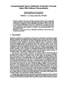
Fig. 1 and 2 depict the finite transition system of the OR1 and OR2 LySa specifications, respectively. The transition system is a graph, in which processes form the nodes and the arcs represent the possible transitions between them. For our present purpose, we just refer to abstract transitions from (label,caption)
state P to state P 0 in the form: P −→ P 0 , where the first part refers to the label of the transition. The second part is only added to recall the reader which part of the protocol the transition represents, e.g. the caption (1 : A −→ B) says that the transition represents the communication between A and B, reported in the first message of protocol. These captures are of no other use. The following are the enhanced labels of the first three transitions of Sys1 discussed above: (i) l1 = hϑA hA, B, N, {A, B, N, NA }KA i, ϑB (A, B; xA N )i, B A )i, , yN (ii) l2 = hϑ0B hA, B, N, {A, B, N, NA }KA , {A, B, N, NB }KB i, ϑS (A, B; yN A (iii) l3 = {A, B, N; wN }.
7
Bodei et al.
The other labels can be computed analogously. A|B|S
l1 ,1:A−→B
A0 | B 0 | S
l2 ,2:B−→S
A0 | B 00 | S 0 l3 ,2:S
dec
A0 | B 00 | S 00 l8 ,4:A dec
l4 ,2:S
dec
A0 | B 00 | S 000 l5 ,3:S−→B
A00 | B | S
l7 ,4:B−→A
A0 | B 0000 | S
l6 ,3:B
dec
A0 | B 000 | S
Fig. 1. Sys1 state transition system.
A|B|S
l10 ,1:A−→B
A0 | B 0 | S
l20 ,2:B−→S
l60 ,4:A dec
A00 | B | S
l50 ,4:B−→A
A0 | B 00 | S 0 l30 ,3:S−→B
A0 | B 0000 | S
l40 ,3:B
dec
A0 | B 000 | S
Fig. 2. Sys2 state transition system.
2.3 Cost Function We now introduce a function $(·) that intuitively assigns costs to individual transitions derived from their labels, alone (see Appendix B for further details). Recall that by “cost” we mean any measure that affects quantitative properties of transitions. In particular, we are interested in cryptographic routines that implement encryptions and decryptions. By inspecting enhanced labels we derive the costs of transitions. The context in which the action occurs, represents a suitable representation of the execution of the run-time support routines leading to that action on the target machine. Following this intuition, we let the cost of the transition depend on both the current action and on its context. Technically, this cost represents the rate of the transition, i.e. the parameter which identifies the exponential distribution of the duration times of the transition. In other words, with “cost” we intend a measure of the time the system is likely to remain within a given transition. Our function therefore specifies the cost of a protocol in terms of the time overhead due to its primitives (see also [16]). In the next sub-section we will perform operations on costs to tune a probabilistic distribution with respect to the expected speed of actions. We intuitively present the main factors that influence costs. 8
Bodei et al. •
The cost of a communication depends on both the input and the output components. Finally, it also depends on its context. · The cost of an output depends on the size of the message and on the cost of each part (or term) of the message. Note that the cost of an encryption is not constant: it depends on the algorithm that implements it, on the size of the cleartext, on the kind of the key (on its size and on its intended use, e.g. long-term or short-term). · The cost of an input depends on the size of the message and on the cost of the terms to be matched. It depends also on the number of checks to make in order to accept the message.
•
The cost of a decryption of a ciphertext depends on the algorithm that implements it, on the size of the ciphertext, on the kind of the key. It depends also on the number of checks to make in order to accept the decryption. To simplify our presentation, we let the cost of a decryption not depend on its context.
Here, we do not fix the cost function: we only propose for it a possible set of parameters that reflect some features of a somewhat idealized architecture and of a particular cryptosystem, e.g. we take into account the number of processors or the kind of cryptographic algorithms. Although very abstract, this suffices to make our point. As discussed before, the context of each action must be considered. Contexts indeed slow down the speed of actions. We therefore determine a slowing factor for any construct of the language. Nevertheless, for simplicity, in our example, we only consider the cost due to parallel composition. •
Parallel composition is evaluated according to the number np of processors available.
•
The cost of restriction depends at least on the number of names n(P ) of the process P because its resolution needs a search in a table of names. Furthermore, it depends on the kind of the name introduced (nonce, longterm key or short-term key).
•
The activation of a new agent via a constant invocation has a cost depending on the size and the number of its actual parameters, as well as on the number of processors available. We do not associate any cost to activations, though.
Example (cont’d) We now associate a cost to each transition in the transition systems in Fig. 1 and 2. For the sake of simplicity, in computing the performance, we neglect the cost due to restrictions. Also, since we can assume that each principal has its own processing unit, we can give cost 1 to each tag ki (i = 0, 1). In other words, we can ignore the context, in our example. Moreover, we give the same cost to output and input. More precisely: •
in a transition representing a communication we assign a cost equal to n ∗ 9
Bodei et al.
c1 = 7s + 4e, c2 = 8s + 4e,
c1 = 3s,
c3 = 4d,
c2 = 4s,
c4 = 4d,
c2 = 8s + 6e,
c5 = 5s + 4e,
c2 = 4d,
c6 = 2d,
c2 = s
c7 = 2s
c2 = 4d.
c8 = 4d; Table 3 Cost Labels in Sys1 (on the left) and Sys2 (on the right).
P s + li=1 mi ∗ e, where n is the size of the message, s denotes the cost of a unitary output, mi is the size of the ith encryption included in the message (if any) and e denotes the cost of a unitary encryption. •
in a transition representing a decryption we assign a cost equal to n ∗ d, where n is the size of the decryption and d denotes the cost of a unitary decryption.
For instance, the cost of the first transition in Fig. 1, carrying label l1 = hϑA hA, B, N, {A, B, N, NA}KA i, ϑB (A, B; xA N )i, is given by (7s + 4e), where 7 are the unary terms used for the output message and 4 is the size of the encrypted cleartext (we assume that input and output have the same cost). The cost of the third transition is instead 4d, that represents the cost of decrypting a ciphertext, obtaining a cleartext of size 4. The full list of the costs ci relative to the labels li in Sys1 and Sys2 are in Tab. 3. Note that cost parameters depend on the platform and on the actual protocol. For instance, in a system where cryptographic operations are performed at very high speed (e.g. thanks to a cryptographic accelerator), but with a slow link (low bandwidth), the cost for encryptions will be low and high for communication. 2.4 Markov Chains Now, we show how to extract quantitative information from a transition system (obtained using our enhanced operational semantics) by transforming it into a CTMC. Our first step is introducing a function that assigns costs to individual transitions, we perform operations on costs. Although we interpret costs as parameters of exponential distributions, our relabeling functions are not intended to manipulate random variables. The intuition is that cost functions define a single exponential distribution by subsequent refinements as soon as information on the run-time becomes explicit. Operationally we start with 10
Bodei et al.
an optimistic selection of an exponential distribution and then, while scanning contexts, we jump to other distributions until the one suitable for the current transition is reached. The cost functions encode this jumping strategy. Once the exponential distributions of transitions have been computed, we make some numerical calculations, possibly by collapsing those arcs that share source and target. Recall that the exponential distributions we use enjoy the memoryless property. Roughly speaking, the occurrence of the next transition is independent of when the last transition occurred. This means that any time a transition becomes enabled, it restarts its elapsing time as if it were the first time that it was enabled. Furthermore, all transitions are assumed to be time homogeneous, meaning that the rate of a transition is independent of the time at which it occurs. We first associate a parameter r with a transition to derive some transition probabilities, defined as the rate at which a system changes from behaving like process Pi to behaving like Pj : it corresponds to the sum of the costs of all the possible transitions from Pi to Pj . Note that in our example, in both transition systems, there is only one transition between each pair of nodes and consequently rates coincide with single costs. Definition 2.1 The transition rate between two states Pi and Pj , written q(Pi, Pj ), is the rate at which the transitions between Pi and Pj occur X q(Pi , Pj ) = $(θk ). θ
k Pi −→P j
Remember that $ is the cost function as defined in Appendix B. A continuous time Markov chain C can be conveniently represented as a directed graph whose nodes are the states of C, and whose arcs only connect the states that can be reached by each other. The rates at which the process jumps from one state to another can be arranged in a square matrix Q, called generator matrix. Apart from its diagonal, it is the adjacency matrix of the graph representation of the of the Continuous Time Markov Chain of the process under consideration (CT MC(P )). The entries of Q are called instantaneous transition rates and are defined by P q(Pi , Pj ) = $(θk ) if i 6= j θk Pi −→Pj (1) qij = n P − if i = j j=1 qij j6=i
Performance measures of systems make sense over long periods of execution. These measures for a process P are then usually derived by exploiting the stationary probability distribution Π for the CTMC we associate with P 11
Bodei et al.
(it exists, because both transition systems are finite and cyclic). Definition 2.2 Let Πt (xi ) = p(X(t) = xi ) be the probability that a CTMC is in the state xi at time t, and let Π0 = (Π0 (x0 ), . . . , Π0 (xn )) be the initial distribution of states x0 , x1 , . . . , xn . Then a CTMC has a stationary probability distribution Π = (Π(x0 ), . . . , Π(xn )) if n X
ΠQ = 0 and
Π(xi ) = 1.
i=0
The stationary distribution for each of the two systems in Fig. 1 and 2, is the solutions of the system of linear equations, defined as above. Note that we can use standard numerical techniques and exploit the preferred numerical package available to make all the computations needed above; the very same for the stochastic analysis, we will make afterwards. Finally, we measure the performance of a process P by associating a reward structure with it, following [11,10,5]. Since our underlying performance model is a continuous time Markov chain, the reward structure is simply a function that associates a value with any state passed through in a computation of P , i.e. with any derivative of P , rather than to each transition, as often done in the literature, e.g. in [14]. For instance, when calculating the utilisation of a cryptosystem, in order to perform a decryption, we assign value 1 to any transition in which the decryption is enabled. All the other transitions earn the value 0 as transition reward. Definition 2.3 Given a function ρθ associating a transition reward with each transition θ in a transition system, the reward of a state P is ρP =
X
ρθ .
θ
P −→Q
Intuitively, the reward structure of a process P is a vector of rewards with as many elements as the number of derivatives of P . From it and from the stationary distribution Π of CT MC of a process P we can compute performance measures. Definition 2.4 Let Π be the stationary distribution of CT MC(P ). The total reward of a process P is computed as R(P ) =
X
ρPi × Π(Pi ).
Pi ∈d(P )
For instance, we obtain the utilisation of a cryptosystem by summing the values of Π multiplied by the corresponding reward structure. This amounts to considering the time spent in the states in which the usage of the cryptosystem is enabled. 12
Bodei et al.
Example (cont’d) Consider again the transition systems in Fig. 1 and 2 which are both finite and have cyclic initial states. These features ensure that they have stationary distributions. We derive the following generator matrices Q1 and Q2 of CT MC(Sys1) and CT MC(Sys2).
b 0 0 0 Q1 = 0 0 0 2d
b g 0 0 0 0 0 0
0 0 0 0 0 0 0 0 0 0 0 0 a 0 0 −2d 2d 0 0 −2s 2s 0 0 −2d 0 0 0 0 0 0 f 0 0 −4d 4d 0 0 −s s 0 0 −4d
0 0 0 g 0 0 −4d 4d 0 0 −4d 4d 0 0 −a 0 0 0 0 0 0 0 0 0
−3s 3s 0 −4s 4s 0 0 −f 0 Q2 = 0 0 0 0 0 0 4d 0 0
The stationary distributions of the Markov chains Πi = (X0 , . . . , Xn−1) (i = 1, 2 and n = 6, 8) for Sys1 and Sys2, solutions of the following systems of linear equations n−1 X ΠQ = 0 and Xi = 1. i=0
are the following: Π1 =
A A A A A A Ai , , , , , , , b 4c 4d 4d a 2d 2s 2d
hA
where: A=
4abcds 6bcs + 4adcs + adbs + 2adbc + 4dbcs
and a = 5s + 4e
b = 7s + 4e c = 2s + e g = 8s + 4e h 4B B 4B B 4B B i Π2 = , , , , , 3s s f d s d
where B=
3df s 20df + 12sd + 6sf
f = 8s + 6e
We compare now the relative efficiency of the two versions of the protocol, in terms of their utilization of cryptographic routines, as discussed above. We assign value 1 (a non-zero transition reward) to any transition in which the decryption is enabled and we assign value 0 to any other transition. In particular, we assign value 1 to the 3rd , 4th , 6th , 8th transitions in Sys1 and to the 4th and 6th transitions in Sys2. 13
Bodei et al.
Using this performance measure, which we call R, we obtain that the performance of OR1 is lower than the one of OR2 , as expected. Indeed 3A 2B R(Sys1) = R(Sys2) = 2d d It is possible to prove that R(Sys1 ) is less or equal to R(Sys2 ), for every positive s, d and e, assuming that encryption and decryption have the same cost. So, we could measure and compare the performance of different versions of the same protocol and establish which is the more efficient.
3
Conclusion
We have presented a framework in which the performance analysis of security protocols, is driven by the semantics of their specifications, given in terms of the process algebra LySa [4]. We used an enhanced operational semantics, whose transitions are labelled by (encodings of) their proofs. Taking advantage of enhanced labels, we mechanically associate rates, i.e probabilistic information, with transitions. This is done symbolically, by looking at the enhanced labels, alone. Actual values are obtained as soon as the user provides some additional information about the architecture and the cryptographic tools relative to the analysed system. Since enhanced labels can be tightly connected to the routines called by the run-time support to implement each operator of the language, the information about architectural features and about algorithms used can be supplied by a compiler. We are particularly interested here in the evaluation of the aspects due to cryptography, such as those depending on the cryptosystem and on the kind of keys used in a particular protocol. This makes it possible to weigh and compare different versions of protocols by the performance point of view. Each cryptosystem implies a different cost that depends on how it consumes resources and time. Furthermore, the algorithm behaviour is influenced by the target platform and vice versa, e.g. in a shared-key architecture where many principals want to communicate each other requires a higher number of different keys than in Client-Server architecture. Therefore our approach makes the critical cost factors evident and helps the designer in choosing efficient solutions. In this paper we have assumed that any activity is exponentially distributed, but general distributions are also possible (see [18]), as they depend on enhanced labels, alone. Once rates have been assigned to transitions, it is easy to derive the CTMC associated with a transition system of a process. From its stationary distribution, if any, we evaluate the performance of the process in hand. Moreover, although many different timing models can be used, in this paper we concentrate on a continuous time approach. It is worth noticing that our approach follows the same pattern presented in [6] to derive behavioural information from our enhanced labels. Also, 14
Bodei et al.
behavioural properties, such as confidentiality and authentication, can be checked by using a tool integrated with ours, like the analyser of LySa [4]. Therefore, we propose our operational semantics as a basis to uniformly carry out integrated behavioural and quantitative analysis. We hope that our proposal is a little step in supporting the designers in the development of applications, by driving and assisting them in error-prone steps such as the translation of a specification into a model, suitable for quantitative analysis.
References [1] M. Abadi and A. D. Gordon. A calculus for cryptographic protocols - The Spi calculus. Information and Computation 148, 1:1–70, January 1999. [2] M. Abadi and R. Needham. Prudent engineering practice for cryptographic protocols In Proc. of IEEE Symposium on Research in Security and Privacy, pp.122–136, IEEE, 1994. [3] A. A. Allen. Probability, Statistics and Queeing Theory with Computer Science Applications. Academic Press, 1978. [4] C. Bodei, M. Buchholtz, P. Degano, F. Nielson, and H. Riis Nielson. Automatic validation of protocol narration. In Proc. of CSFW’03, pages 126–140. IEEE, 2003. [5] G. Clark. Formalising the specifications of rewards with PEPA. In Proc. of PAPM’96, pp. 136-160. CLUT, Torino, 1996. [6] P. Degano and C. Priami. Non Interleaving Semantics for Mobile Processes. Theoretical Computer Science, 216:237–270, 1999. [7] P. Degano and C. Priami. Enhanced Operational Semantics. ACM Computing Surveys, 33, 2 (June 2001), 135-176. [8] DES. Fed. Inform. Processing Standards. Data encryption standard., 1977, Pub.46, National Bureau of Standards, Washington DC, January. [9] H. Hermanns and U. Herzog and V. Mertsiotakis. Stochastic process algebras – between LOTOS and Markov Chains. Computer Networks and ISDN systems 30(9-10):901-924, 1998. [10] J. Hillston. A Compositional Approach to Performance Modelling. Cambridge University Press, 1996. [11] R, Howard. Dynamic Probabilistic Systems: Semi-Markov and Decision Systems, Volume II, Wiley, 1971. [12] R. Milner, J. Parrow, and D. Walker. A calculus of mobile processes (I and II). Info. & Co., 100(1):1–77, 1992.
15
Bodei et al.
[13] R. Nelson. Probability, Stochastic Processes and Queeing Theory. SpringerVerlag, 1995. [14] C. Nottegar, C. Priami and P. Degano. Performance Evaluation of Mobile Processes via Abstract Machines. IEEE Transactions on Software Engineering, 27(10):867-889, Oct 2001. [15] D. Otway and O. Rees. Efficient and timely mutual authentication. ACM Operating Systems Review, 21(1):8–10, 1987. [16] A. Perrig and D.Song. A First Step towards the Automatic Generation of Security Protocols. Proc. of Network and Distributed System Security Symposium, 2000. [17] G. Plotkin. A Structural Approach to Operational Semantics, Tech. Rep. Aarhus University, Denmark, 1981, DAIMI FN-19 [18] C. Priami. Stochastic π-calculus with general distributions. PAPM’96, pp.41-57. CLUT Torino, 1996.
In Proc. of
[19] A. Reibnam and R. Smith and K. Trivedi. Markov and Markov reward model transient analysis: an overview of numerical approaches. European Journal of Operations Research: 40:257-267, 1989. [20] W. J. Stewart. Introduction to the numerical solutions of Markov chains. Princeton University Press, 1994. [21] K. S. Trivedi. Probability and Statistics with Reliability, Queeing and Computer Science Applications Edgewood Cliffs, NY, 1982.
A
Enhanced Operational Semantics of
LySa
The syntax of LySa consists of terms E and processes P , where N and X denote sets of names and variables, respectively. Encryptions are tuples of terms E1 , · · · , Ek encrypted under a term E0 representing a shared key. Values, that correspond to closed terms, i.e. terms without free variables, are used to code keys, nonces, messages etc. , E ::= terms ∈ E n
name (n ∈ N )
x
variable (x ∈ X )
{E1 , · · · , Ek }E0 symmetric encryption (k ≥ 0) 16
Bodei et al.
P ::= processes ∈ P 0
nil
hE1 , · · · , Ek i. P
output
(E1 , · · · , Ej ; xj+1 , · · · , xk ). P input (with matching) P1 | P2
parallel composition
(ν n)P
restriction
A(y1 , . . . , yn )
constant definition
decrypt E as {E1 , · · · , Ej ; xj+1 , · · · , xk }E0 in P symmetric decryption (with matching) The set of free variables/free names, written fv(·)/fn(·) and α-equivalence ≡α are defined in the standard way. As usual we omit the trailing 0 of processes and use the standard notion of substitution: P [E/x] is the process P where the occurrences of x are replaced by E. Here, hE1 , · · · , Ek i and (E1 , · · · , Ej ; xj+1 , · · · , xk ) represent the output and the input prefix, respectively. At run-time prefixes contain closed terms (apart from the variables xj+1 , · · · , xk ). To denote run-time prefixes we will use the meta-variables µout and µin , resp. in the following. Our enhanced operational semantics for LySa is built on the top of a reduction semantics. As usual, processes are considθ ered modulo structural congruence ≡. The reduction relation −→ is the least relation on closed processes, i.e. processes with no free variables, that satisfies the rules in Table A.1. We first focus on the actions (similar to the standard semantics) and afterwards on the new form of processes and on the labels that enrich transitions. The rule (Com) expresses that an output hE1 , · · · , Ej , Ej+1 , · · · , Ek i. T is matched by an input (E10 , · · · , Ej0 ; xj+1 , · · · , xk ).T 0 in case the first j elements are pairwise the same. When the matchings are successful each Ei is bound to each xi . Similarly, the rule (Decr) expresses the result of matching the term resulting from an encryption {E1 , · · · , Ej , Ej+1 , · · · , Ek }E0 , against the pattern inside the decryption decrypt E as {E10 , · · · , Ej0 ; xj+1 , · · · , xk }E00 in T : the first j components should be the same, additionally, the keys must be the same, i.e. E0 = E00 — this models perfect symmetric cryptography. When successful, each Ei is bound to each xi . The rules (Par), (Res) and (Congr) are standard. Finally, P (a1 , . . . , an ) is the definition of constant (hereafter a ˜ denotes the sequence a1 , . . . , an ). Each agent identifier A has a unique defining equation of the form A(y1 , . . . , yn ) = P , where the yi are distinct and fn(P ) ⊆ {y1 , . . . , yn }. Hereafter, we will restrict ourselves to processes that generate finite state spaces, i.e. which have a finite set of derivatives. 5 Note 5
A sufficient condition for a process to be such is that all the agent identifiers occurring in
17
Bodei et al.
that this does not mean that the behaviour of such processes is finite, because their transition systems may have loops. Indeed, particular forms of loops are essential to apply the steady state analysis that we carry out in our examples. The above ensures that our processes have a finite set of derivatives. (Com) ∧ji=1 Ei = Ei0 ϑ||i ϑO hE1 , · · · , Ek i T | {z } |
hout,ini
out
−→ T | T 0 [Ej+1 /xj+1 , · · · , Ek /xk ]
ϑ||1−i ϑI (E10 , · · · , Ej0 xj+1 , · · · , xk ) T 0 |
{z
}
in
(Decr)
∧ji=0 Ei = Ei0 decrypt ({E1 , · · · , Ek }E0 )
hdeci
as {E10 , · · · , Ej0 ; xj+1 , · · · , xk }E 0 in T −→ T [Ej+1 /xj+1 , · · · , Ek /xk ] {z }0 | dec
(Par)
(Res)
(Ide) :
θ
T0 −→ T00 θ
(ν n)T −→ (ν n)T 0
T0 | T1 −→ T00 | T1
θ
T −→ T 0
T {˜ a/˜ y } −→ T 0
θ
A(˜ a) −→ T 0
θ
θ
, A(˜ y) = T
(Congr) θ
T ≡ T0 ∧ T0 −→ T1 ∧ T1 ≡ T 0 θ
T −→ T 0 Table A.1 θ Proved Operational semantics, T −→ T 0 .
For the (proved) operational semantics of the our calculus, we need to associate to each transition an enhanced label in the style of [6,7]. An enhanced label records: the action corresponding to the transition and the syntactic context in which the action takes place, in particular to the input and output part of a communication. To associate the context to each component, we statically associate a context label ϑ to each prefix of a given process. Mainly, these labels take into account the parallel composition and the restriction construct (by distinguishing which kind of name the restriction creates). Technically, we use two functions: the first B distributes context labels on a given process and the second T builds the label, by introducing a k0 (resp. k1 ) for the left (resp. it have a restricted form of definition A(˜ y ) = P . Namely, A can occur in P only if prefixed by some action and cannot occur within a parallel context.
18
Bodei et al.
for the right) branch of a parallel composition and a νa for each restriction of the name a. In the end, we will have a new kind of processes LP, ranged over by T, T 0 , where each prefix is associated by a context label. Definition A.1 Let L = {k0 , k1 } with χ ∈ L∗ , O = {νa , νK , νN } 3 o. Then the set of context labels is then defined as (L ∪ O)∗ , ranged over by ϑ. Definition A.2 (Distributing labels) − ϑB0 = 0 − ϑ B (ϑ0 µ.T ) = ϑϑ0 µ.(ϑ B T ) − ϑ B T0 | T1 = (ϑ B T0 ) | (ϑ B T1 ) − ϑ B (νa)T = (νa) ϑ B T − ϑ B A(y1 , . . . , yn ) = A(y1 , . . . , yn ) −ϑ B decrypt {E1 , · · · , Ek }E0 as {E10 , · · · , Ej0 ; xj+1 , · · · , xk }E00 in T = decrypt {E1 , · · · , Ek }E0 as {E10 , · · · , Ej0 ; xj+1, · · · , xk }E00 in ϑ B T We can now define the function T mapping processes from P in LP. Definition A.3 Let A, B be standard processes and let B the operator introduced in the previous definition. The following is a bijection: − T ((νa)T ) = (νa)νa B T (T ) − T (T0 |T1 ) = k0BT (T0 ) | k1BT (T1 ) − T (0) = 0 − T (µ.T ) = µ.T (T ) − T (A(y1 , . . . , yn )) = A(y1 , . . . , yn ) − T (decrypt E as {E1 , · · · , Ej ; xj+1 , · · · , xk }E0 in T ) = decrypt E as {E1 , · · · , Ej ; xj+1 , · · · , xk }E0 in T (T ) We need the following structural congruence rule to distribute the restriction labels to parallel processes: (νa)(νa B T0 )|T1 ≡ (νa)(νa B T0 |νa B T1 ) Now, we are ready to introduce the enhanced labels of transitions. Note that in the first label (the one relative to communication), there is a common part between the input and the output contexts. Definition A.4 The set Θ of enhanced labels, ranged over θ, is defined by θ ::= hϑk1−i ϑO µO , ϑki ϑI µI i|h{E10 , · · · , Ej0 ; xj+1 , · · · , xk }E00 i | {z } | {z } | {z } out
in
dec
19
Bodei et al. ϑ
Labelled transitions −→ are introduced in (Com) and (Dec). The reϑ duction −→ is closed under the other inference rules (parallel composition, constant invocation, restriction and congruence rule). To recover the original reduction semantics that, by definition, does not use labels, it is sufficient to eliminate them and to eliminate context labels from processes.
B
Cost function
We are going to formally define the function which associates a cost with each transition labelled by θ. This cost represents the rate of the transition, i.e. the parameter which identifies the exponential distribution of the duration times of θ. Therefore the cost of each component of an enhanced label ϑµ depends on the action µ and on the context ϑ. To define a cost function, we start by considering the execution of the action µ on a dedicated architecture that only has to perform µ, and we estimate once and for all the corresponding duration with a fixed rate r. Then we model the performance degradation due to the run-time support. In order to do that, we introduce a scaling factor for r in correspondence with each routine called by the implementation of the transition θ under consideration. We proceed now with our definitions. First we assign costs to the composition of terms (in particular of encryptions), and to the components of actions µin , µout . The functions fu (n) and fu (n) represent the cost of unary terms, the functions, while fenc represents the cost function for the encryption (computing the cost of the routines that implement the encryption algorithm). The cost function of a tuple coincides with the minimum cost among the costs of each component, to reflect the speed of the slower operation. Moreover, the functions fin , fout define the costs of the routines which implement the send and receive primitives, where the function f= (j) represents the cost function for a pattern matching of size j. In the following, fkind (crypt) denotes the cost of an encryption or a decryption, due to the cryptosystem used; similarly for fkind (EO ) denotes the cost due to the choice of a particular key (depending on the size and the intended use). Moreover, for fsize (ctxt) denotes the cost due to the size of the cleartext to encrypt. Furthermore, fsize (msg) stands for the cost due to size of the message to send or to receive in the evaluation of the cost of an output or an input. Finally, f= (j) is the function that computes the cost of performing a pattern matching on j terms. •
$T (n) = fu (n)
•
$T (x) = fu (x)
•
$T ({E1 , . . . , En }E0 ) = fenc (fkind (crypt), fsize (ctxt), fkind (EO ), $T (E1 , . . . , Ek ))
20
Bodei et al. •
$T ((E1 , . . . , En )) = min($T (E1 ), . . . , $T (En ))
•
$in (µin ) = fin (fsize (msg), f= (j), $T (E1 , . . . , Ej ))
•
$out (µout ) = fout (fsize (msg), $T (E1 , . . . , Ek ))
According to the intuition that contexts slow down the speed of actions, we now determine a slowing factor for any construct of the language. The idea is to devise a general framework in which real situations The cost of the operators is expressed by the function $o (ki ) = fk (np), i = 0, 1 $o ((νa)) = fν (n(P ), fkind (a)) Parallel composition is evaluated according to the number np of processors available. A particular case is $o (k) = 1 which arises when there is an unbound number of processors. (Recall that we are not yet considering communications.) The cost of restriction depends at least on the number of names n(P ) of the process P because its resolution needs a search in a table of names. Furthermore, it depends on the kind of the name fkind (a) (nonce, long-term key, short-term key). Let the label of the transition in hand be hϑ||iϑin µin , ϑ||1−iϑout µout i. The two partners perform independently some low-level operations locally to their environment. These operations are recorded in ϑin and ϑout , inductively built by the application of the function T . Each of the tags of ϑi leads to a delay in the rate of the corresponding µi , which we compute through the auxiliary cost function $o . Then the pairing h||i ϑin µin , ||1−iϑout µout i occurs and corresponds to the actual communication. Since communication is synchronous and handshaking, its cost is the minimum of the costs of the operations performed by the participants independently to make communications reflect the speed of the slower partner. Recall indeed that the lower the cost, the greater the time needed to complete an action and hence the slower the speed of the transition occurring. 6 We estimate the corresponding duration with a fixed rate r = min{$in (||iϑin µin ), $out (||1−iϑout µout )}. Finally, there are those operations, recorded in ϑ, that account for the common context of the two partners. If the label is hdeci, then the cost is the one computed with the function fdec , that corresponds to the cost of the routines that implement the decryption algorithm, including the cost of pattern matching. We now have all the ingredients to define the function that associates costs with enhanced labels. It is defined by induction on θ and by using the auxiliary 6
An exponential distribution with rate r is a function F (t) = 1 − e−rt , where t is the time parameter. The value of F (t) is smaller than 1 and limt→∞ F (t) = 1. The shape of F (t) is a curve which monotonically grows from 0 approaching 1 for positive values of its argument t. The parameter r determines the slope of the curve. The greater r, the faster F (t) approaches its asymptotic value. The probability of performing an action with parameter r within time x is F (x) = 1 − e−rx , so r determines the time, ∆t, needed to have a probability near to 1.
21
Bodei et al.
functions $µ as basis, and then $o . Definition B.1 Let the cost function, where i = 0, 1, can be defined as $(µ) = $µ (µ) $(oθ) = $o (o) × $(θ) $(ki θ) = $o (ki ) × $(θ) $(hϑki ϑin µin , ϑk1−i ϑout µout i) = $(ϑ) × min{$(ki ϑin µin ), $(k1−i ϑout µout ) $(hdeci) = fdec (fkind (crypt), fsize (ctxt), f= (j), fkind (EO ), $T (E1 , . . . , Ej ))
22