1College of Marine Science, University of South Florida, St. Petersburg,. Florida, USA. 2Rosenstiel School of Marine and Atmospheric Science, University of. Miami, Miami ... different training methods, not on the quality of the map- pings or the ...
JOURNAL OF GEOPHYSICAL RESEARCH, VOL. 111, C05018, doi:10.1029/2005JC003117, 2006
Performance evaluation of the self-organizing map for feature extraction Yonggang Liu,1 Robert H. Weisberg,1 and Christopher N. K. Mooers2 Received 22 June 2005; revised 22 December 2005; accepted 3 February 2006; published 25 May 2006.
[1] Despite its wide applications as a tool for feature extraction, the Self-Organizing Map
(SOM) remains a black box to most meteorologists and oceanographers. This paper evaluates the feature extraction performance of the SOM by using artificial data representative of known patterns. The SOM is shown to extract the patterns of a linear progressive sine wave. Sensitivity studies are performed to ascertain the effects of the SOM tunable parameters. By adding random noise to the linear progressive wave data, it is demonstrated that the SOM extracts essential patterns from noisy data. Moreover, the SOM technique successfully chooses among multiple sets of patterns in contrast with an Empirical Orthogonal Function method that fails to do this. A practical way to apply the SOM is proposed and demonstrated using several examples, including long time series of coastal ocean currents from the West Florida Shelf. With improved SOM parameter choices, strong current patterns associated with severe weather forcing are extracted separate from previously identified asymmetric upwelling/downwelling and transitional patterns associated with more typical weather forcing. Citation: Liu, Y., R. H. Weisberg, and C. N. K. Mooers (2006), Performance evaluation of the self-organizing map for feature extraction, J. Geophys. Res., 111, C05018, doi:10.1029/2005JC003117.
1. Introduction [ 2 ] Our understanding of ocean processes steadily improves with increasing information obtained from in situ and remotely sensed data [such as from moored Acoustic Doppler Current Profilers (ADCP), satellite sea surface temperature (SST), sea surface height (SSH), and Chlorophyll, and high-frequency radar sampling of surface currents], and numerical models. However, the percentage of data actually used is low, in part because of a lack of efficient and effective analysis tools. For instance, it is estimated that less than 5% of all remotely sensed images are ever viewed by human eyes [Petrou, 2004]. With the increasing quantity of data there is a need for effective feature extraction methods. [3] Temporal and spatial averaging are the simplest methods, but it is difficult to define suitable time and length scales over which to average. For example, currents on a continental shelf may exhibit different isotropic or anisotropic behaviors depending on the processes and timescales involved [Liu and Weisberg, 2005]. Thus mean values may be very misleading. [4] The Empirical Orthogonal Function (EOF) analysis technique is useful in reducing large correlated data sets into an often much smaller number of orthogonal patterns ordered by relative variance, with wide oceanographic and meteorological applications [e.g., Weare et al., 1976; Klink, 1 College of Marine Science, University of South Florida, St. Petersburg, Florida, USA. 2 Rosenstiel School of Marine and Atmospheric Science, University of Miami, Miami, Florida, USA.
Copyright 2006 by the American Geophysical Union. 0148-0227/06/2005JC003117$09.00
1985; Lagerloef and Bernstein, 1988; Espinosa-Carreon et al., 2004]. However, conventional EOF, as a linear method, may not be as useful in extracting nonlinear information [Hsieh, 2001, 2004]. [5] The Self-Organizing Map (SOM), based on an unsupervised neural network [Kohonen, 1982, 2001], appears to be an effective method for feature extraction and classification. It maps high-dimensional input data onto a lowdimensional (usually 2-d) space while preserving the topological relationships between the input data. Thousands of SOM applications are found among various disciplines [Kaski et al., 1998; Oja et al., 2002], including climate and meteorology [Hewitson and Crane, 1994, 2002; Malmgren and Winter, 1999; Cavazos, 2000; Ambroise et al., 2000; Hsu et al., 2002; Hong et al., 2004, 2005] and biological oceanography [Ainsworth, 1999; Ainsworth and Jones, 1999; Silulwane et al., 2001; Richardson et al., 2002; HardmanMountford et al., 2003]. Recent SOM applications include SST and wind pattern extractions from satellite data [Richardson et al., 2003; Risien et al., 2004; Liu et al., 2006] and ocean current pattern extractions from moored ADCP data [Liu and Weisberg, 2005]. All of these applications suggest that the SOM may be useful for meteorological and oceanographic feature extraction. However, for meteorologists and oceanographers unfamiliar with neural network techniques, the SOM remains a ‘‘black box,’’ with associated skepticism. [6] Early evaluations of SOM performance focused on comparisons with other techniques, such as principal component analysis and k-means clustering [Murtagh and Hernandez-Pajares, 1995; Kiang and Kumar, 2001]. In an introduction to the SOM Toolbox [Vesanto et al., 1999,
C05018
1 of 14
C05018
LIU ET AL.: EVALUATION OF SOM IN FEATURE EXTRACTION
C05018
Figure 1. A 3 � 4 SOM representation of the linear progressive wave data. The top 12 plots show the SOM patterns with the frequency of occurrence given at the top of each plot. The bottom plot is the BMU time series. 2000] performance tests were only on the computational requirements of the algorithms, i.e., computing time for different training methods, not on the quality of the mappings or the sensitivity to different SOM parameter choices. [7] Here we attempt to evaluate the performance of the SOM in feature extraction by using time series generated from known patterns along with sensitivity tests under various tunable parameter choices and signal-to-noise levels. Some of the questions addressed are: does the SOM technique recover known patterns reliably, are any artifices created, and which parameter choices provide the ‘‘best results?’’ Given these findings from synthetic data sets, we then apply the approach to an actual data set consisting of observed current velocity profiles. [8] The remainder of this paper is arranged as follows. Section 2 introduces the SOM. In section 3, time series of linear progressive wave data are used to train and evaluate the SOM method. The results of using various map sizes, lattice structures, initializations, and different neighborhood
functions are tested against a control run. By adding random noise to the known time series, the capability of the SOM in extracting essential features from noisy data is also examined. Section 4 considers a more complex synthetic data set consisting of multiple patterns and compares SOM extractions with those by EOF. The SOM is then applied to an oceanographic data set in section 5. Section 6 concludes with a summary and discussion.
2. Brief Introduction to the SOM [9] The SOM performs a nonlinear projection from the input data space to a set of units (neural network nodes) on a two-dimensional grid. Each unit has a weight vector mi, which may be initialized randomly. Here the unit number i varies from 1 to M, M being the size of the SOM array. Adjacent units on the grid are called neighbors. In the Matlab SOM Toolbox [Vesanto et al., 2000] there are three types of training algorithms: sequential, batch, and sompak.
2 of 14
C05018
LIU ET AL.: EVALUATION OF SOM IN FEATURE EXTRACTION
C05018
data set is partitioned into M groups (by minimum Euclidian distance) and each group is used to update the corresponding weight vector. Updated weight vectors are calculated by: mi ðt þ 1Þ ¼
M X nj hij ðt Þxj j¼1
, M X nj hij ðt Þ
ð3Þ
j¼1
where xj is the mean of the n data vectors in group j. The hij(t) denotes the value of the neighborhood function at unit j when the neighborhood function is centered on the unit i. In the batch algorithm, the learning rate function a(t) of the sequential algorithm is no longer needed, but, like the sequential algorithm, the radius of the neighborhood may decrease during the learning process. Inthe SOM Toolbox, there are four types of neighborhood functions available: ‘‘bubble,’’ ‘‘gaussian,’’ ‘‘cutgauss,’’ and ‘‘ep’’ (or Epanechikov function).
hci ðt Þ ¼
Figure 2. Same as Figure 1 but for a 2 � 2 SOM. [10] In a sequential training process, elements from the high-dimensional input space, referred to as input vectors x, are presented to the SOM, and the activation of each unit for the presented input vector is calculated using an activation function. Commonly, the Euclidian distance between the weight vector of the unit and the input vector serves as the activation function. The weight vector of the unit showing the highest activation (i.e., the smallest Euclidian distance) is selected as the ‘‘winner’’ [or best matching unit (BMU)]. This process is expressed as ck ¼ arg min k xk � mi k
ð1Þ
where ck is an index of the ‘‘winner’’ on the SOM for a data snapshot k, and c varies from 1 to M. The ‘‘arg’’ denotes ‘‘index.’’ During the training process the weight vector of the winner is moved toward the presented input data by a certain fraction of the Euclidean distance as indicated by a time-decreasing learning rate a. Also, the weight vectors of the neighboring units are modified according to a spatialtemporal neighborhood function h. The learning rule may be expressed as mi ðt þ 1Þ ¼ mi ðt Þ þ aðt Þ � hci ðt Þ � ½xðt Þ � mi ðt Þ ;
ð2Þ
where t denotes the current learning iteration and x represents the currently presented input pattern. This iterative learning procedure leads to a topologically ordered mapping of the input data. Similar patterns are mapped onto neighboring units, whereas dissimilar patterns are mapped onto units farther apart. [11] The batch version of the SOM algorithm is computationally more efficient than the sequential version [Kohonen, 1998; Vesanto et al., 1999, 2000]. At each step of the training process, all the input data vectors are simultaneously used to update all the weight vectors. The
8 Fðst � dci Þ > > > > > � � > > > exp �dci2 =2s2t
> > exp �dci =2st Fðst � dci Þ cutgauss > > > n o > > : max 0; 1 � ðs � d Þ2 ep t ci
ð4Þ
where st is the neighborhood radius at time t, dci is the distance between map units c and i on the map grid and F is a step function Fð x Þ ¼
8