performance limitation of neural network model for wind ... - IEEE Xplore
Recommend Documents
AbstractâVisual area V4 lies in the middle of the ventral visual pathway in the primate brain. It is an intermediate stage in the visual processing for object ...
to the central limit theorem, the pdf can be approximated by a .... is asymptotically efficient; it reaches the Cramer–Rao bound ..... Oxford, U.K.: Basil Blackwell,.
In this paper, we present a new architecture of solving model predictive control (MPC) problem based on one layer recurrent neural network. We give algorithm ...
Sep 15, 2017 - and the constraints should be twice differentiable. Since sparse ... Index Termsâ Lagrange programming neural networks. (LPNNs), locally ...
Logic Based MPPT Techniques for Solar PV Systems. Ankit Gupta, Pawan Kumar, Rupendra Kumar Pachauri, Yogesh K. Chauhan. Electrical Engineering ...
mutual comparison between rule-based expert system and artificial neural network in predicting flow stress of a commonly used type of steel. The prediction ...
1Brno University of Technology, Speech@FIT, Czech Republic. 2 Department of Electrical and Computer Engineering, Johns Hopkins University, USA. {imikolov ...
network reconfiguration for service restoration are investigated in this paper. ... simulation was conducted on the 69-bus distribution system. Index terms ...
Florida Institute of Technology. Department of Electrical and Computer Engineering. 150 W. University Blvd., Melbourne Fl. 32901, USA. Abstract - The problem ...
AbstractâIn this paper, a neural network (NN)-based method- ology is developed for the motion control of mobile manipulators subject to kinematic constraints.
*CINVESTAV del IPN, Unidad Guadalajara. Av. del Bosque, Col. El BajÃo, Zapopan, Guadalajara, Jalisco 45019, MEXICO email: [email protected].
load forecaster using artificial neural network (ANN) models. Three approaches have been undertaken to forecast the load demand up to. 24 hours ahead.
Neural network approach for determination of fatigue crack depth profile in a metal, using alternating current field measurement data. M. Ravan, S.H.H. Sadeghi ...
AbstractâIn this paper, the usage of artificial neural networks. (ANN) for the estimation of the direction-of-arrival (DOA) in an OFDM-based MIMO configuration ...
Modular Artificial Neural Network for Prediction of. Petrophysical Properties From Well Log Data. Chun Che Fung, Member, IEEE, Kok Wai Wong, Member, IEEE, ...
Abstract: To explore the main components of the future computing machines, the spiking neurons for feature extraction and dimensionality reduction applications ...
Nov 9, 2015 - Coimbatore, Tamil Nadu 641 046, India ... Attribution License, which permits unrestricted use, distribution, and reproduction in ... Hindawi Publishing Corporation ... prediction protects the generation of secured wind power and.
Sep 4, 2014 - 3Defence Research and Development Canada, Suffield Research Centre, Medicine Hat, Alberta, Canada. 4School of Renewable Energy, ...
AbstractâIn this paper we present a framework for evaluating wireless network performance through emulation. The frame- work uses a hybrid design in which ...
planning, standards development, and the potential areas of research. .... ROW GOY^ ([email protected]) is a senior software engineer at Nexabit. Networks ...
Page 1. 2834. IEEE TRANSACTIONS ON CYBERNETICS, VOL. 44, NO. 12, DECEMBER 2014. Neural-Network-Based Online HJB Solution for. Optimal ...
systems, as an alternative to the conventional analytical methods. The aims of the paper .... of high-voltage transmission lines, several software tools have been ...
neural network (ANN) in predicting the occurrence of lightning events based on historical lightning and meteorological data. ANN, which was inspired by the way ...
performance limitation of neural network model for wind ... - IEEE Xplore
autoregressive terms in a neural network model with specific reference to an application to wind turbine condition monitoring. The model's ability to detect ...
Neural Network Modelling with Autoregressive Inputs for Wind Turbine Condition Monitoring Y. Wang*, D.G. Infield † *University of Strathclyde, Email: [email protected] University of Strathclyde, Email: [email protected]
Abstract Artificial neural networks enjoy popularity among different areas of modelling, including financial decision making, medical diagnosis, visualisation, and process control. This paper presents potential problems with the inclusion of autoregressive terms in a neural network model with specific reference to an application to wind turbine condition monitoring. The model’s ability to detect anomalies is explored by employing 10-minute supervisory control and data acquisition (SCADA) data from a commercial wind turbine gearbox. The issues associated with the inclusion of autoregressive inputs are assessed through an investigation of the weighting parameters for each neuron in the hidden and output layers and the outputs from these neurons.
1 Introduction The current trend in Europe is increasingly towards installing wind capacity offshore where the wind speeds are higher and there are less environmental concerns. Wind turbine condition monitoring can play an essential role in improving O&M and delivering improved turbine availability and thus economic viability. Reference [8] provides a recent review of turbine condition monitoring techniques for different components and sub-systems. Compared with vibration analysis and oil debris analysis, both of which require expensive sensors, data mining techniques based on data already available from the turbine control system (SCADA data) are more cost effective and have the potential to provide useful insights into the condition and operational health of a wide range of wind turbine components, and also the turbine itself in terms of its overall power generation performance.. Among all the data mining techniques, artificial neural networks are widely employed for wind turbine condition monitoring due to their ability to model nonlinear dynamic process and efficiently resolve pattern recognition issues [7, 11]. References [12] and [14] both present successful wind turbine gearbox fault diagnosis examples using neural network models with a three-layer structure. The former identifies gearbox anomalies through model learning and comparison with turbine performance data based on gearbox cooling oil temperature taken from SCADA data, and the
latter employs 9 vibration signals from a gearbox, in vertical, horizontal and axial directions, as model inputs. Despite of its robustness in nonlinear statistical identification and relationship learning, care is required during model construction and training. Issues such as local minima in gradient descent algorithm and extrapolation limitations in model estimation have already gained awareness for different neural network model applications. Reference [1] investigates the local minima issue in neural networks using the back propagation algorithm and proposes some sufficient conditions for robust solutions. Reference [6] provides an insight into the neural network model structure and gives an explanation of its limited extrapolation capability. Besides the common issues mentioned above, the neural network model also suffers from performance limitation with specific reference to models including autoregressive inputs. The main purpose for introducing autoregressive lag terms in a time series of variable is to feed information to current or future value estimation from historical records [4]. The success of Markov modelling underpins this approach. Successful identifications of incipient turbine anomalies are demonstrated in both [15] and [5], both of which employ autoregressive inputs. Effect of autoregressive inputs inclusion on model performance is investigated in this paper based on the identical NN model presented in reference [15].
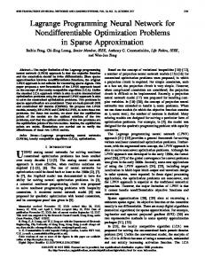
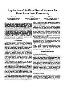
2 Neural network background Neural network models, being biologically inspired, are parametric models designed to capture data interrelationships between input parameters and outputs using weight and bias parameters for individual neurons. These weights are established through a training process, often using the back propagation algorithm. Figure 1 shows an example of multilayer feed-forward neural network consisting of input layer, hidden layer and output layer, each of which comprises a group of neurons. It should be noted that although the hidden layer could consist of more than one layer, only three-layer neural networks (i.e. one hidden layer) is discussed in this paper due to its popularity. Figure 2 illustrates the inner structure of an elementary neuron where R represents the number of elements in input vector. W and b are weight vector and bias of the neuron, respectively. The weighted sum is then input into a transfer function ݂ to generate neuron output ܽ, which is fed as input
to the neurons in next layer until reaching the output layer. The most commonly used three transfer functions for multilayer neural network model are log-sigmoid transfer function, the tan-sigmoid transfer function and linear transfer function, the algebraic algorithms and corresponding graphs of which are tabulated as follows.
techniques to iteratively adjust the weights and biases in each neuron, the recurrent neural network models have achieve a significant breakthrough in model accuracy and have become the most popular neural network learning strategy [16]. A list of either gradient or Jacobin based algorithms with their detailed descriptions for recurrent neural network training is presented in [2]. Among all the training functions provided, the Levenberg-Marquardt algorithm is claimed to be the fastest algorithm for small networks, but not so appropriate for large networks due to its requirement of more memory and computation time.
Log-sigmoid transfer function ܽ ൌ ݈݃݅ݏ݃ሺ݊ሻ ൌ
ͳ ͳ ݁ ି
Figure 1: Neural network model architecture example Tan-sigmoid transfer function ܽ ൌ ݃݅ݏ݊ܽݐሺ݊ሻ ൌ
Figure 2: Inner structure of a general neuron with R inputs Figure 1 shows an example of multilayer feed-forward neural network consisting of input layer, hidden layer and output layer, each of which comprises a group of neurons. It should be noted that although the hidden layer could consist of more than one layer, only three-layer neural networks (i.e. one hidden layer) is discussed in this paper due to its popularity. Figure 2 illustrates the inner structure of an elementary neuron where R represents the number of elements in input vector. W and b are weight vector and bias of the neuron, respectively. The weighted sum is then input into a transfer function ݂ to generate neuron output ܽ, which is fed as input to the neurons in next layer until reaching the output layer. The most commonly used three transfer functions for multilayer neural network model are log-sigmoid transfer function, the tan-sigmoid transfer function and linear transfer function, the algebraic algorithms and corresponding graphs of which are tabulated as follows. Unlike the feed-forward neural network where all information flow transmits uni-directionally from inputs node to outputs, the recurrent neural network involves feedback loops in the training process, and hence data is allowed to transmit bidirectionally [13]. And by utilizing the back propagation
ʹ െͳ ͳ ݁ ିଶ
Linear transfer function ܽ ൌ ݈݊݅݁ݎݑሺ݊ሻ ൌ ݊
Table 1: Three commonly used transfer functions As is shown in Figure 1, the number of neurons in the input and output layers is determined by the number of input and output variables that are relevant for a given problem, hence these are treated as fixed in model construction. There are some discussions ongoing regarding how many neurons should be chosen for the hidden layer. The general rule is that the neuron number should not be too large as this can lead to over-fitting of the model and cause failure to model generalization, and also not too small as this will result in model under-fitting. Reference [10] suggests the hidden layer size should to be between one-half and three times the inputs size, and reference [3] proposes an optimal hidden neuron of 75% of the input variables number, neither of which is commonly accepted due to insufficient theoretical supports. In practice, the decision of optimal hidden layer size involves experience and experiment [9].
3 Case study and discussions Reference [6] explains the reason behind a particular model’s inability to extrapolate by investigating the output from individual neurons. Following the same methodology, a model that attempts to forecast the cooling oil temperature of a wind turbine gearbox is investigated based on 10-minute SCADA data. The same model architecture of 4-2-1 as employed in references [15] is utilized in this paper. The model consists of four inputs, one output and two neurons in the hidden layer, with the tan-sigmoid transfer function being used for each individual neuron in the hidden and output layer. Therefore, the neuron output from the hidden and output layers can be expressed as follows. ͳ݊݁݀݀݅ܪൌ ݃݅ݏ݊ܽݐሺࢄ ȉ ࢃுௗௗଵ ܾுௗௗଵ ሻ
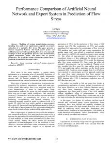
Where X indicates the input row vector, and parameter b and column vector W have the same meanings as introduced in Figure 2, with subscript ‘Hidden1’, ‘Hidden2’ implying the first and second neurons in the hidden layer and ‘Output’ implying the output layer. Four inputs including output power, nacelle temperature and two latest historical records (autoregressive inputs) of model output are illustrated in Figure 3 below.
Figure 3: Gearbox cooling oil temperature model architecture Matlab neural network toolbox is utilized to train the model, which is then applied to the validating and testing data. The issue caused by autoregressive inputs is analysed by statistical and graphical investigation of trained model and the model’s capability of anomaly detection is explored by using the testing results. 3.1 Model training Three months of healthy wind turbine operational data are used in the training process. Consistent with the previous section, the Levenberg-Marquardt algorithm is utilized for back propagation in model training. The model so obtained is then analysed by investigating neuron parameters including weight vector values and bias. Table 2 below lists the values of neuron parameters in both the hidden and output layers as assigned during the training process. The weight vectors for the hidden layer neurons correspond to model inputs in the same order as shown in Figure 3.
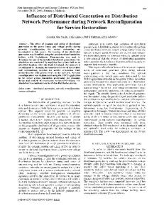
Table 2: neuron parameters for hidden and output layer Firstly, it should be noted that the 1st neuron in the hidden layer is making no effective contribution to the output as it is permanently saturated (see Figure 5(a) below), so no importance need be attached to its weighting values. Secondly, it is noticeable that in the second hidden neuron, the autoregressive inputs were assigned weights of the order of ͳͲିଷ , but much smaller weights (even down to ͳͲି ) were assigned to the other (heterogeneous) parameters. This implies that the autoregressive inputs dominate and that the contributions from other input variables will tend to be relatively small. In this particular set-up, a purely autoregressive model may well turn out to be the best available for forecasting oil temperature and thus it may be reasonable for the training process to give low weights to the heterogeneous variables. However, such a scheme would have essentially no ability to detect anomalous behavior and it remains to be seen whether other combinations of variables would discriminate better between normal and anomalous behavior. To illustrate the problem caused by introducing autoregressive inputs, time series of training data for three variables are presented in Figure 4 below. Figure 5 shows the corresponding neurons’ outputs from the hidden and output layers, calculated based on Equations (1), (2) and (3). The neuron parameters are presented in Table 2. A very similar time series trend can be observed in Figures 4(b) and 5(b) in spite of their different scales. The first hidden neuron keeps a constant output value of 1, which is caused by transfer function saturation, and thus does not contribute to the model’s output. Consequently, the final output follows the second hidden neuron alone and produces a ‘desired result’. The concern is about the extent to which this is effectively a time-shifted copy of the autoregressive inputs as a result of these terms dominating the output of that neuron. Further investigation takes the form of model validation, and is the subject of the next section.
power training input
training hidden layer node1 output
600
0 -0.2
500
-0.4 400
-0.6 -0.8
kw
300
-1 200
-1.2 -1.4
100
-1.6 0
-1.8 -100
0
2000
4000
6000
8000
10000
12000
-2
0
4(a): Power output
2000
4000
6000
8000
10000
12000
10000
12000
10000
12000
5(a): 1st neuron in hidden layer
cooling oil temperature training input 60
training hidden layer node2 output 0.94
50
0.945 0.95
degree Celsius
40
0.955
30 0.96
20
0.965 0.97
10
0.975
0
0
2000
4000
6000
8000
10000
12000
0.98
0
4(b): Gearbox cooling oil temperature
2000
4000
6000
8000
5(b): 2nd neuron in hidden layer
nacelle training input 35
training target 60
30
50
degree Celsius
25
40
20
30
15
10
20
5
10 0
0
2000
4000
6000
8000
10000
12000
4(c): nacelle temperature
Figure 4: Training data time series for input variables
0
0
2000
4000
6000
8000
5(c): Neuron in output layer
Figure 5: Neuron output from hidden and output layer
3.2 Model validating
gearbox cooling oil temperature (degree Celsius)
70 observations model estimations
60
50
40
30
20
10
0
0
500
1000
1500 2000 2500 3000 time series (10min per point)
3500
4000
4500
6(a): Model with four inputs
gearbox cooling oil temperature (degree Celsius)
70 observations model estimations
60
50
Data from one month of healthy, fault free operation are used here for model validation. Result obtained from the model, trained as described in the last section, is shown in Figure 6(a). It is compared with results from two simpler models, one being set-up with only two autoregressive inputs (shown in Figure 6(b)) and the other having only the heterogeneous variables, power output and nacelle temperature (shown in Figure 6(c)). The models maintain the same number of hidden nodes and are retrained accordingly. The first two figures show excellent agreement between model estimations and observations, suggesting that the autoregressive terms dominate as anticipated, and that the heterogeneous inputs contribute little. This would seem to provide further evidence that the model performance is achieved in the main through simple persistence forecasting rather than reflecting possible relationships across the input domain. However, the model testing case in next section will shows that the situation is more complicated. Figure 6(c) shows that a model without the autoregressive terms does not follow the data at all well, particularly during periods of non-operation, highlighting the need for a more extensive set of input variables, perhaps including in this specific case the gearbox bearing temperature and generator rotational speed as these are available in the SCADA database.
40
3.3 Model testing and anomaly detection 30
20
10
0
0
500
1000
1500 2000 2500 3000 time series (10min per point)
3500
4000
4500
6(b): Model with only two autoregressive inputs
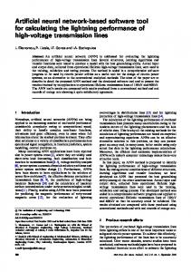
One month data prior to a confirmed turbine gearbox failure is utilized as testing data and the corresponding results are illustrated in Figure 7. In this case, Figure 7(a), the original four-input model shows significant differences between the modelled temperature and the data (i.e. residuals) which indicate potential turbine anomaly. In contrast, the model with only two autoregressive inputs, shown in Figure 7(b), simply acts as a persistence model, following the measured data perfectly but with a time lag, and thus is incapable of anomaly detection.
Figure 7: Model testing results It should be noted that the maximum oil temperature in the training dataset is 53.7Ԩ, which is smaller than the peak oil temperature measurement (64.9 Ԩ ) in the testing dataset presented in Figures 7. The maximum temperature modelled using the full set of inputs (Figure 7(a)) at this peak is 60.5Ԩ demonstrating that the proposed model is capable of extrapolation beyond the maximum training value, although with uncertain accuracy.
4 Conclusion The neural network model with autoregressive inputs is capable of wind turbine anomaly detection. However the reasons behind this for a model that is constructed with heavily weighted autoregressive terms remain uncertain. The model is able to extrapolate outside of the value range of the training data but the accuracy of such extrapolation in unclear and of potential concern. These issues need to be further explored. Due to the issues discussed, caution is required regarding input parameter selection during neural network model construction in order to achieve a valid and reliable model. Future work will deal with the improvement of model performance that could be achieved by both increasing the size of training data to minimise extrapolation issues and extending the range of input variables to include more heterogeneous model-related parameters.
References [1] M. Bianchini, M. Gori and M. Maggini, On the Problem of Local Minima in Recurrent Neural Networks, IEEE Transactions on Neural Networks, Vol. 5, No. 2, pp. 167-177, Mar. 1994. [2] M.H. Beale, M.T. Hagan and H.B. Demuth, Neural Network ToolboxTM User’s Guide, The Math Works, Version 7, Sep 2010. [3] D. Baily and D.M. Thompson, Developing Neural Network Applications, Al Expert, Sep. 1990.
[4] J.D. Cabedo, I. Moya, Estimating Oil Price ‘Value at Risk’ Using the Historical Simulation Approach, Energy Economics, Vol. 25, Issue 3, May 2003. [5] M.C. Garcia, M.A. Sanz-Bobi, and J.D. Pico, Aug. 2006, SIMAP: Intelligent System for Predictive Maintenance: Application to Health Condition Monitoring of a Wind Turbine Gearbox, Computers in Industry, Vol. 57, pp.552568. [6] P.J. Haley and D. Soloway, Extrapolation Limitations of Multilayer Feedforward Neural Networks, International Joint Conference on Neural Network, Vol. 4, pp. 25-30, 1992. [7] S. Haykin, Neural Networks: A Comprehensive Foundation, IEEE Press,1994. [8] Z. Hameed, Y.S. Hong, Y.M. Cho, S.H. Ahn and C.K. Song, Condition Monitoring and Fault Detection of Wind Turbines and Related Algorithms: A Review, Renewable and Sustainable Energy Reviews, Vol.13, pp. 1-39, 2009. [9] I. Kaastra and M. Boyd, Designing A Neural Network for Forecasting Financial and Economic Time Series, Neurocomputing, Vol. 10, pp. 215 -236, 1996. [10] J.O. Katz, Developing Neural Network Forecasters for Trading, Technical Analysis of Stocks and Commodities, pp. 58-70, Apr. 1992. [11] A. Munoz, M.A. Sanz-Bobi, An Incipient Fault Detection System Based on the Probabilistic Radial Basis Function Network, Application to the diagnosis of the condenser of a coal power plant, Neurocomputing 23, pp. 177–194, 1988. [12] R. F. Mesquita Brandão, J. A. Beleza Carvalho and F. P. Maciel Barbosa, Neural Networks for Condition Monitoring of Wind Turbines, Modern Electric Power Systems, Poland, 2010. [13] A. Raj, G. Bincy and T. Mathu, Survey on Common Data Mining Classification Techniques, International Journal of Wisdom Based Computing, Vol. 2(1), Apr. 2012. [14] S. Yang, W. Li and C. Wang, The intelligent fault diagnosis of wind turbine gearbox based on artificial neural network, International Conference on Condition Monitoring and Diagnosis, pp. 1327-1330, 2008. [15] A. Zaher, S.D.J. McArther, D.G. Infield, and Y. Patel, Online Wind Turbine Fault Detection through Automated SCADA Data Analysis, Wind Energy, Vol. 12, pp. 574-593, Sep. 2009. [16] A. Zaher, Automated Fault Detection for Wind Farm Condition Monitoring, A thesis submitted for the degree of Doctor of Philosophy, University of Strathclyde, Sep. 2010.