Performance Modeling and Stability of Semi-Persistent ... - CiteSeerX

4446

IEEE TRANSACTIONS ON WIRELESS COMMUNICATIONS, VOL. 11, NO. 12, DECEMBER 2012

Performance Modeling and Stability of Semi-Persistent Scheduling with Initial Random Access in LTE Jun-Bae Seo, Member, IEEE, and Victor C. M. Leung, Fellow, IEEE

Abstract—In this paper we examine the feasibility of semipersistent scheduling (SPS) for voice over IP (VoIP) by random access and evaluate its performance in terms of throughput of random access and traffic channels, and random access delay. We further investigate system stability issues and present methods to stabilize the system. To see the VoIP capacity gain, we show the maximum number of acceptable VoIP terminals without exceeding some front-end packet dropping (i.e., voice clipping) probability. In addition, we examine the effect of the parameter called implicit release after in the LTE standard on the system performance, which is used for silence period detection. Our performance evaluation model based on Equilibrium Point Analysis is compared to simulations. Index Terms—Multiaccess communication, access protocol, cellular networks, communication system signalling, algorithm design and analysis.

I. I NTRODUCTION

L

ONG Term Evolution (LTE) has emerged as a candidate for fourth generation (4G) cellular networks, which will meet the anticipated explosive demands on wireless bandwidth by providing peak data rates of 300 Mbps over downlink with 4 × 4 multi-input multi-output (MIMO) antennas and 75 Mbps over uplink. In order to use these radio resources efficiently, LTE adopts two scheduling mechanisms. The first one is dynamic scheduling, which allocates radio resources dynamically based on each terminal’s buffer status and radio channel state information. The size of resources together with the modulation and coding scheme (MCS) would be allocated to meet some quality of service (QoS) requirements. To support this algorithm, terminals must send to eNodeB (a base station in LTE) certain uplink reporting messages either via a random access channel, or via some dedicated control channels in order to inform eNodeB of associated buffer status and channel quality. Although this algorithm is expected to improve total radio resource utilization in the provisioning of QoS for each terminal, it could consume substantial control signaling overhead, particularly for traffic with small and periodic packets that are semi-static in size, e.g., Voice over IP

Manuscript received December 20, 2011; revised April 28 and August 29, 2012; accepted September 10, 2012. The associate editor coordinating the review of this paper and approving it for publication was D. Tarchi. This work was supported by the Canadian Natural Sciences and Engineering Research Council through a postgraduate scholarship and grant RGPIN 44286-09. The authors are with the Department of Electrical and Computer Engineering, the University of British Columbia, Vancouver, BC V6T 1Z4 Canada (e-mail: {jbseo, vleung}@ece.ubc.ca). Digital Object Identifier 10.1109/TWC.2012.100112.112254

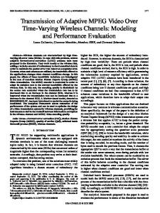
(VoIP) or Transmission Control Protocol (TCP) acknowledgement (ACK) packets. The second mechanism is called semipersistent scheduling (SPS), which allocates an uplink traffic channel periodically without any additional control message during a traffic burst, e.g., the ON period of a VoIP traffic stream. At the beginning of an SPS operation, an initial uplink traffic channel is obtained either by random access or via an assigned control channel, over which a periodic reservation is made. When an assigned control channel is used for reserving a traffic channel at the beginning of SPS operation, a scheduling request indicator (SRI) based on on/off keying is transmitted first in an assigned control channel, called the physical uplink common control channel (PUCCH) [1]. Then eNodeB allocates an uplink grant that allows the terminal to send a buffer status reporting message as shown in Fig. 1. Finally eNodeB grants a traffic channel to the terminal. When the SRI is not sent over PUCCH, Hybrid Automatic Repeat reQuest (H-ARQ) Acknowledgement (ACK) and negativeACK (NACK), and radio channel quality indicator (CQI) can share this PUCCH. While SPS with SRI over PUCCH can reduce channel set-up times significantly, PUCCH for SRI may be wasted during long inactive periods of an application. On the other hand, when a terminal has lost time-synchronization during an inactive period, it is mandatory to perform random access at the beginning of the next SPS operation. In SPS, the allocated traffic channel would be implicitly released when a certain number of empty transmission slots are found on the allocated traffic channel. This number is called ‘implicit release after’, which is specified as either 2, 3, 4 or 8 [2]. Note that, in the SPS operation, the size of resources and MCS are not changed, once they are allocated at the beginning of SPS. The allocation interval of the traffic channel is called the ‘SPS interval in uplink’, which is specified as either 10, 20, 32, 40, 64, 80, 128, 160, 320 or 640 subframes [2]. It is expected that VoIP traffic would typically use an SPS interval of 20 subframes [1], while other intervals might be used according to the uplink traffic characteristics. Hereafter, we denote the values of ‘implicit release after’ and ‘SPS interval in uplink’, by K and L, respectively. In SPS operation for VoIP traffic, K is used for detecting and confirming an ensuing silence period, or can help to hold the reserved traffic channel to prevent it from being released due to some packets being lost over the radio channel. However, a large K could cause low throughput of the reserved traffic channels. As previous work, Rinne et al. [3] provide a simulation study of Evolved Universal Terrestrial Radio Access (E-

c 2012 IEEE 1536-1276/12$31.00 

SEO and LEUNG: PERFORMANCE MODELING AND STABILITY OF SEMI-PERSISTENT SCHEDULING WITH INITIAL RANDOM ACCESS IN LTE

UTRA) for VoIP and best effort (BE) traffic streams, in which the standards of physical and medium access layers are considered in detail. Particularly, SPS operation is compared with a fully dynamic scheduling algorithm with and without packet bundling1, while round robin and proportional fair channeldependent scheduling algorithms are considered for BE traffic together with MIMO and some MCSs. In [4] Bi et al. consider that terminals use signalling channels at the beginning of VoIP talk spurts in an OFDMA system in order to obtain a traffic channel and then transmit VoIP packets in the reserved traffic channels once the signalling message would be granted, which is close to SPS with SRI. While SPS in LTE can be used for VoIP traffic as well as possibly uplink web traffic, VoIP traffic scheduling algorithms have also been developed for IEEE 802.16 systems2 [5]-[7], which is another candidate for 4G networks. Particularly when VoIP traffic changes its state from OFF to ON, the scheduling algorithms in [5][6] allocate the radio resource to the VoIP traffic by dedicated control channel in conjunction with polling, which also shows some resemblances to SPS algorithm with SRI, while [7] considers a random access for the resource allocation. In contrast with SPS with SRI in LTE introduced before, we propose SPS with initial random access where a traffic channel is reserved by random access at the beginning of SPS operation in order to complement SPS with SRI, and examine the feasibility of SPS with initial random access with respect to how many VoIP terminals can be allowed provided that their random access delay does not exceed a predefined delay constraint. Compared to previous work [3][4] focusing on the physical layer performances of VoIP scheduling algorithm with dedicated control channel, the feasibility of our scheme is expected to improve VoIP capacity without consuming additional dedicated control channels and also leads to flexible use of SPS parameters such as K and L for various traffic characteristics. To this end, we characterize the performance of SPS with initial random access based on K in terms of the traffic channel throughput, random access delay, and packet dropping probability. Our contributions are summarized as follows. 1) We characterize the system performance in terms of random access throughput and delay, traffic channel throughput, and packet dropping probability with a given delay constraint. Based on these performance metrics, VoIP capacity can be found as the number of terminals admitted without violating a predefined packet dropping probability. 2) By simulations and analysis we examine system stability in terms of the probability distribution of the number of backlogged terminals in the system, when the uniform backoff (UB) algorithm is applied over the random access channel. We then show how to mitigate bistability of the system. 1 In packet bundling, multiple VoIP packets are bundled based on channel quality and then transmitted together over the downlink by a dynamic scheduler. 2 As in LTE, IEEE 802.16 systems are also based on orthogonal frequency division multiple access (OFDMA), in which some subcarriers are used for random access channels. Particularly, both systems employ a demandassignment multiple access protocol consisting of 4-way handshaking procedure.

4447

Fig. 1. Signal flow of SPS with Scheduling Request Indicator (SRI) or with random access.

The remainder of this paper is organized as follows. We introduce SPS with random access and make some assumptions in Section II. In Section III we analyze this system by using Equilibrium Point Analysis (EPA) [8] as an approximation. Our analysis is compared against simulations in Section IV. Concluding remarks are given in Section V. II. M ODELS AND A SSUMPTIONS A. Random Access for SPS Algorithm In an LTE radio frame, each physical random access channel (PRACH) occupies six radio resource blocks (RBs) in the frequency domain, where each radio RB is formed by 12 subcarriers. The PRACH appears periodically, as specified by the PRACH configuration index. For instance, one PRACH is found every two subframes when the PRACH configuration index is 12 [9]. At most one PRACH is allowed in a subframe, while only one PRACH is available in the frequency domain of a slot. Note that, in an LTE frequency division duplexing (FDD) frame structure, each 10 msec frame consists of 10 subframes, and each subframe consists of two slots. Thus, the length of one slot is 0.5 msec, which corresponds to one packet transmission time. Each accessing terminal randomly chooses one of 64 orthogonal random access preambles (RAPs) called Zadoff-Chu sequences and transmits it over a PRACH. Some of the RAPs would be directly allocated by eNodeB to some terminals for contention-free random access. In SPS with initial random access, contention-based random access is used for reserving a traffic channel that is periodically allocated to a terminal. Suppose that P RAPs are available for contentionbased random access. First the requesting terminal selects one of P RAPs at random and transmits it with initial power F in a PRACH. When multiple terminals transmit the same RAP in the same PRACH, a RAP collision occurs. Secondly, eNodeB broadcasts the random access response (RAR) on the downlink control channel within a predefined time-window as shown in Fig. 1. From the RAR message the successful terminals obtain the backoff parameter U , timing advance command, the RAP identifier and the reserved uplink RBs. If a requesting terminal cannot find its RAP identifier, it regards itself as backlogged and increases its RAP transmission counter by one. If the counter is equal to the maximum number of allowed RAP transmissions, denoted by RL , the terminal drops its RAP retransmission and reports this to the higher layer. Otherwise, the terminal selects a random backoff time between 0 and U (msec), and delays its retransmission by the selected backoff time. When a terminal retransmits a RAP, it increases the

4448

IEEE TRANSACTIONS ON WIRELESS COMMUNICATIONS, VOL. 11, NO. 12, DECEMBER 2012

RAP transmission power by ΔF , subject to the constraint that the RAP transmission power cannot exceed Fmax . This is called the power ramping scheme, which is repeated up to the maximum of allowed RAP transmissions until the terminal transmits a RAP successfully. Third, a terminal finding its RAP identifier in the RAR message transmits a message called Msg3 [2] via H-ARQ conveying information such as a radio resource control (RRC) connection request, or tracking area update. We assume that the terminal’s buffer status reporting in Fig. 1 could be transmitted via Msg3 in SPS with random access. If this message is successfully transmitted, eNodeB finally allocates a traffic channel to the requesting terminal, which it will use periodically. Based on the random access procedure above [2][9], our assumptions are summarized as follows: A1) We assume that there are M terminals in this system, each of which has an infinite queue to store incoming VoIP packets. A2) Since LTE has various PRACH configurations, as an example we assume that one slot consists of one PRACH and D OFDMA subcarriers for user traffic, with each slot corresponding to one packet transmission time. A3) We assume perfect orthogonality among RAPs transmitted in the PRACH, i.e., no multiple access interference occurs between different RAPs. Therefore, the LTE random access channels can be regarded as a multichannel SALOHA system. Although the standard includes a power ramping scheme for RAP transmissions over the PRACH, we do not take power ramping into account to keep our model simple and tractable. A4) In practice, when a RAP collision occurs, all the terminals that transmitted the same RAP will receive the same traffic channel to transmit SR requests. The eNodeB allows the RAP-colliding terminals to simultaneously transmit an Msg3 in the channel allocated to all of them [2], with the expectation that the resulting collision on this channel would be resolved by HARQ. If terminals cannot transmit Msg3 successfully up to the maximum of retransmissions of HARQ, they will repeat the RAP transmission. We simplify our model by not taking into account of Msg3 transmissions via HARQ. Moreover, we conservatively assume that a RAP collision destroys all transmissions involved and the corresponding terminals retransmit randomly selected RAPs based on UB algorithm after RAR reception. We further assume that a terminal gets an uplink traffic channel right after successful RAP transmission, skipping the Msg3 transmission. In fact, an Msg3 transmission after a successful RAP transmission merely adds a deterministic delay to the random access delay. A5) For a terminal transmitting a unique RAP, i.e., successful RAP transmission, its random access cannot be declared as successful if there is no traffic channel available for assignment to it. In this paper, a random access is said to be successful, when a terminal receives a traffic channel assignment after successful RAP transmission. Thus, a successful random access (different from a successful RAP transmission) is the synonym of a successful traf-

fic channel reservation. Accordingly, the random access delay is defined as the time that is taken for a terminal to reserve a traffic channel successfully, after it transmits the first RAP. Furthermore, we assume that terminals get feedback on success or failure of random access, just after RAP (re)transmissions, without any error, i.e., right before the beginning of the next slot. A6) Compared to UB algorithm with retry limit [2], our analytical model uses UB algorithm with infinite retransmissions, RL = ∞. However, our simulation model implements the UB algorithm with retransmission limit for a better representation of a real system. A7) In addition to A5, if the number of terminals successfully transmitting RAPs, say z, is greater than the number of available traffic channels, say d, eNodeB randomly chooses d among z terminals and allocates them d traffic channels. Then, z − d terminals will be backlogged due to the lack of available traffic channels and will perform the backoff algorithm in A6, i.e., these terminals suffer from a reservation blocking. B. Uplink Traffic Model When each VoIP packet is generated every 20 msec by an adaptive multi-rate (AMR) voice codec at 12.2 kbps [1], a total of 50 packets/sec are generated with the payload size of 31 bytes. We approximately model this VoIP traffic stream by a two-state Markov-modulated Bernoulli process (MMBP) [10]. We assume that in every slot a traffic source that is in the OFF-state may change its state to the ON-state with probability 1 − β, and a traffic source that is in the ONstate may change its state to the OFF-state with probability 1 − α. This assumption gives average ON and OFF periods as 1/(1 − α) and 1/(1 − β) (slots), respectively. We further assume that one packet is always generated at the transition from the OFF-state to the ON-state, while a packet is generated every slot based on a Bernoulli trial with probability σ during the rest of the ON period. As in [11], we assume the average ON and OFF periods to be 1000 and 1350 (msec), which respectively correspond to α = 0.999 and β = 0.9993 for 1 msec slot. We also set σ = 0.05, which represents a 20 msec average inter-arrival time of VoIP packets during the ON periods. Particularly, we assume that after a terminal has reserved a traffic channel by random access, no more than one packet can be generated in the ON state during each transmission period of L + 1 slots. C. Semi-Persistent Scheduling in LTE We begin by summarizing in Table I the symbols used in describing SPS with initial random access. Recall that, after a terminal successfully reserve a traffic channel via random access, it transmits its VoIP packets in the allocated traffic channel every L + 1 slots. During this period, no more packets are generated in the ON-state. Thus, packet arrivals in the ON state of our MMBP model depend on the terminal’s reservation state. An allocated traffic channel is implicitly released, when K consecutive empty transmissions are observed in the allocated traffic channel. After the reserved traffic channel has been released, the terminal should perform

SEO and LEUNG: PERFORMANCE MODELING AND STABILITY OF SEMI-PERSISTENT SCHEDULING WITH INITIAL RANDOM ACCESS IN LTE

4449

TABLE I S YMBOLS USED IN SPS ALGORITHM WITH INITIAL RANDOM ACCESS Notation P M U L K D σ α (β) ci n f t0 (t1 ) (k) rij

RES(LK,0)

RES(Lk,0)

RES(L1,)0

RES(21,)0

RES(LK,1)

RES(Lk,1)

RES(L1,)1

RES(21,1)

RES

(k ) 0, 3

RES

(1) L,2

● ● ● ● ● ●

RES

(k ) L,2

● ● ● ● ● ●

RES

(K ) 0, 2

● ● ● ● ● ●

RES

(K ) L,2

● ● ● ● ● ●

RES

( K 1) 0, 2

Definition Number of orthogonal random access preambles Total number of terminals Window size of uniform backoff algorithm SPS interval in uplink. Allocated data channel appears every L + 1 slots Implicit release after. Maximum of allowed empty transmissions on an allocated traffic channel Number of data channels The probability that a packet is generated in the ON state in slot The probability of VoIP traffic source being in the ON (OFF) state in a slot Number of backlogged terminals with window size i Number of terminals with ON state of VoIP traffic source Number of terminals with OFF state of VoIP traffic source Number of terminals in the transmission state, when VoIP traffic source is in ON (OFF) state (k) Number of terminals with a reserved traffic channel. The indexes, k, i and j correspond to Rij

RES1(1,0)

TX0 RES

(1) 2, 2

(1) 1, 3

RES

TX1 RES0( K,31)

RES(LK,3)

N RES2

Fig. 2.

RES(0K,3)

N RES3

RES(Lk,3)

CONU

RES(L1,)3

RES(0k, 4)

CONU 1

● ● ●

RES(21,)3

CON1

RES1(1, 4)

CON0

State transition diagram of terminals with SPS algorithm with random access.

random access again when it needs to send more VoIP packets. This system (i.e., SPS with initial random access) can be regarded as an extension of the packet reservation multiple access (PRMA) in [11], which is based on S-ALOHA for traffic channel reservations. Compared to PRMA with P = D = K = 1, where a permission probability is used as a backoff algorithm, terminals in our system reserve a traffic channel by multichannel S-ALOHA (P ≥ 1, D ≥ 1, and K ≥ 1) and use UB algorithm to recover from collisions. Fig. 2 shows the possible states of each terminal with respect to the random access, which can be explained as follows: 1) A terminal’s uplink traffic source behaves every slot based on MMBP model in Section II-B. When the terminal has not started the random access to reserve a traffic channel, the state of the terminal is depicted by the NRES2 - and the NRES3 state in Fig. 2, which corresponds to the ON and OFF state of the traffic source, respectively. Note that even for the NRES2 in Fig. 2, no packet is available for transmission (as MMBP may not generate a packet). While the terminal does not have a reserved traffic channel, the arrival of a VoIP

packet (this can occur after an extended silence during the ON-state of VoIP source, or due to a transition from the OFF- to the ON-state of VoIP source) causes the terminal to contend for a traffic channel assignment by accessing the random access channel. This moves the terminals state to one of the contention states (CONi for 0 ≤ i ≤ U ) based on the UB algorithm with delayed first transmission. 2) Once a terminal enters the CONi state for reserving a traffic channel, for simplicity we assume that its VoIP source state stays in the ON state until a successful random access, as a VoIP source is unlikely to change its state during the signalling delay in [4]. Every slot a terminal in the CONi state moves into the CONi−1 state with probability one, according to the UB algorithm. Note that, while a terminal is in the CONi state for 0 ≤ i ≤ U , new packets can be generated. This will be discussed in detail in Sections III-B. Terminals in the CON0 state will select a RAP randomly and transmit it in the PRACH. 3) When a terminal has successfully reserved a traffic

4450

IEEE TRANSACTIONS ON WIRELESS COMMUNICATIONS, VOL. 11, NO. 12, DECEMBER 2012

channel, it moves from the CON0 state into the traffic transmission state, denoted by the TX0 state. The TX1 state indicates the traffic transmission state in which the terminal’s voice traffic is in the OFF state. 4) During L subsequent slots after the TX0 or the TX1 state, the terminal is said to be in the i-th reservation (k) state, which is denoted by the RESi,j for 1 ≤ i ≤ L and 1 ≤ k ≤ K (this superscript denotes the counter of the empty transmissions). Note that during these states the terminal can have a packet in the ON state of VoIP source, and some slots later VoIP source goes to the OFF state. Accordingly, the subscript j = 0 (1) denotes the ON (OFF) state of VoIP traffic source with a packet, while j = 2 (3) denotes the ON (OFF) state without a packet. (k) 5) Finally, the RES0,j state for 2 ≤ k ≤ K +1 and j = 2, 3 represents an empty transmission on the traffic channel reserved for a terminal, which can be reached from the (k−1) RESL,j state without a packet arrival for j = 2, 3. III. A NALYSIS A. Equilibrium Point Analysis Based on Fig. 2, we denote the numbers of terminals in the (k) NRES2 -, the NRES3 -, the TX0 -, the TX1 -, the RESi,j - and (k) the CON states by N , F , T0 , T1 , Ri,j and C (called the state variables), respectively. The state space of this system (k) is represented by {C for 0 ≤  ≤ U , T0 , T1 , N, F, R1,j (k) for 1 ≤ k ≤ K and j = 0, 2, 3, Ri,j for 1 ≤ k ≤ K, (k) 2 ≤ i ≤ L and 0 ≤ j ≤ 3, R0,j for 2 ≤ k ≤ K + 1, j = 2, 3}. If a multidimensional Markov chain is considered to describe M terminals’ states, the number of possible states could be as large as M 2+U+1 (D + 1)K(5+4(L−1))+2 states (k) in Fig. 2, in which T0 , T1 and Ri,j take the value from 0 to D. Typically we use M ≥ 70, U ≥ 10, L = 20, K ≥ 1 and D = 5 in Section IV. Instead of finding a joint probability of M terminals’ states, by using EPA we focus on the number of terminals in a specific state when the system is in equilibrium, i.e., steady state. In what follows, we first obtain a system equilibrium function denoted by F (c0 ), in which c0 is the number of terminals in the CON0 state in equilibrium. This equilibrium function shows the difference between the inflow, i.e., the number of terminals, from the (K+1) (K+1) states to the NRES2 -, the RES0,2 - and the RES0,3 NRES3 -, or the CONi state for 0 ≤ i ≤ U (releasing the traffic channel reservation) and the outflow of the CON0 state (reserving the traffic channel) in Fig. 2. If the difference is zero at some c0 , the system is said to be in equilibrium. One can skip the following lengthy derivations through (1)-(29) and directly find F (c0 ) in (30). The system performance metrics are obtained by (31)-(35) in terms of random access delay, throughput, and packet (front-end) dropping probability. In order to find F (c0 ), we denote the equilibrium value of each state variable by small letters, c , t0 , t1 , n, f , (k) ri,j , respectively. Additionally, we define the following row  (k) (k) (k) (k)  vectors, t = [t0 t1 ], r1 = r1,0 0 r1,2 r1,3 for 1 ≤ k ≤ K,  (k) (k) (k) (k)  (k) ri = ri,0 ri,1 ri,2 ri,3 for 1 ≤ k ≤ K and 2 ≤ i ≤ L,  (k) (k)  (k) r0 = r0,2 r0,3 for 2 ≤ k ≤ K + 1. Based on A2, the

state transitions occur at slot boundaries. By assuming that the expected flow into and out of each state variable are equal [8], we construct the following state balance equations: First, (k) at the RESi,j state for 1 ≤ k ≤ K and 0 ≤ j ≤ 3, we have (k)

r1

(k)

= t Hk−1 g,

r2

ˆ = t Hk−1 g h

(1)

for 3 ≤ i ≤ L,

(2)

and (k)

ri

ˆ hi−2 = t Hk−1 g h

ˆ hL−2 u0 , and the matrices, g and h, ˆ are in which H = g h respectively expressed as   σα 0 (1 − σ)α 1 − α g= (3) 1−β 0 0 β and

⎡

1−α 0 0 0 0 (1 − σ)α 0 0

α ⎢ 0 ˆ ⎢ h=⎣ σα 1−β

⎤ 0 0 ⎥ ⎥. 1−α ⎦ β

(4)

(1) In (1), for instance, r1 = t g indicates that the number of terminals in the TX0 - and the TX1 state moves to one of the (1) RES1,j state for j = 0, 2, 3 with probability g. The matrices h and u0 are expressed as ⎡ ⎤ α 1−α 0 0 ⎢ 1−β β 0 0 ⎥ ⎥ (5) h=⎢ ⎣ σα 0 (1 − σ)α 1 − α ⎦ 1−β 0 0 β

and

⎡

0 ⎢ 0 u0 = ⎢ ⎣ (1 − σ)α 0 (k+1)

(6)

state for j = 2, 3, we can write

For the RES0,j

(k+1)

r0

⎤ 0 0 ⎥ ⎥. 1−α ⎦ β

= t Hk

for k = 1, 2, · · · , K.

(7)

We denote by Λ (r, c0 ) the number of packets which successfully reserve the remaining traffic channels by random access, given total of r currently reserved traffic channels and c0 terminals at the CON0 state. We can get the total number of reserved traffic channels r by r=

K k=1

(k)

rL e4 = t

K

k−1  ˆ L−2 e4 , H g hh

(8)

k=1

in which en represents a unit column vector whose length is n. At the TX0 - and the TX1 state we can write t0 =

K k=1

(k)

rL u◦1 + Λ (r, c0 )

and t1 =

K

(k)

rL u•1 ,

(9)

k=1

in which the column vectors, u◦1 and u•1 , are expressed as ⎡ ⎡ ⎤ ⎤ α 1−α ⎢ 1−β ⎥ ⎢ β ⎥ • ⎢ ⎥ ⎥ u◦1 = ⎢ (10) ⎣ σα ⎦ and u1 = ⎣ 0 ⎦ . 1−β 0

SEO and LEUNG: PERFORMANCE MODELING AND STABILITY OF SEMI-PERSISTENT SCHEDULING WITH INITIAL RANDOM ACCESS IN LTE

Referring to Fig. 2, the left hand side and right hand side in (9) respectively indicate the expected flow out of t0 (or t1 ) and into t0 (or t1 ). Using (1), we can rewrite t1 in (9) as t1 = t

K

ˆ L−2 u• ⇒ t1 = a0 t0 + a1 t1 , Hk−1 g hh 1

from which we have t1 = a0 /(1 − a1 )t0 . Note that the constants a0 and a1 are numerically determined. We then express t in terms of t0 as t = t0 w, 

(12)

in which we have w  = [1 a0 /(1 − a1 )]. By substituting (12) into (8), we can get r by K

k−1  ˆ L−2 e4 . r  r(t0 ) = t0 w  g hh H

(13)

In (9) we can get Λ(r, c0 ) by c0

mr (z)Γ(z|c0 , P ),

+ c0 − Λ(r, c0 ) = cU .

(19)

At the CONi state for 0 ≤ i ≤ U − 1 we also get    1   (K+1) (K+1) + (1 − β) f + r0,3 σα n + r0,2 U +1  + c0 − Λ(r, c0 ) + ci+1 = ci .

(14)

z=1

in which mr (z) = min(z, max(D − r, 0)) is the conditional mean of successfully reserved traffic channels by random access, which is based on A7. We denote the binomial probability distribution

 function with parameters b, L and p by B(b, L, p) = Lb (p)b (1 − p)L−b . Further, Γ(z|c0 , P ) is the probability that z among c0 terminals select a unique RAP given total of P RAPs, according to A3. We can obtain recursively Γ(z|k, P ) by [13]

(20)

Using (19) we can rewrite ci for 0 ≤ i ≤ U    U + 1 − i  (K+1) (K+1) ci = + (1 − β) f + r0,3 σα n + r0,2 U +1  + c0 − Λ(r, c0 ) .

k=1

Λ(r, c0 ) =

At the CONU state we get    1   (K+1) (K+1) + (1 − β) f + r0,3 σα n + r0,2 U +1 

(11)

k=1

4451

(21)

At the CON0 state we then have     (K+1) (K+1) + (1 − β) f + r0,3 = Λ(r, c0 ), σα n + r0,2 (22) in which the left hand side indicates the expected flow into the backlog states, i.e., CONi for 0 ≤ i ≤ U , while Λ(r, c0 ) indicates the expected output flow from the CON0 state. After some tedious manipulation on (17)-(22), we have (K+1)

r0,2

(K+1)

+ r0,3

= Λ(r, c0 ) ⇒ t0 wH  K e2 = Λ( r (t0 ), c0 ), (23)

in which (13) has been used. Eq. (23) means that the flow out (K+1) (K+1) of the RES0,2 - and the RES0,3 state is equal to the flow out of the CON0 state. If we can express (23) as a function of c0 only, we can solve for c0 that satisfies (23). Thus, we only k Γ(z|k, P ) = B(m, k, 1/P )Γ(z − I(m − 1)|k − m, P − 1) need to express t0 as a function of c0 . To this end, we use the fact that the sum of the number of terminals distributed over m=0 (15) each state should be equal to M , which is expressed as in which I(x) is one at x = 0 and zero elsewhere. The above equation has the following initial conditions: Γ(0|1, 0) = 1,

t e2 +

L K

(k)

ri e4 +

k=1 i=1

U

ci + n + f = M.

i=0

Due to fluid approximation of EPA, c0 is a real number for 0 ≤ c0 ≤ M in (14), which makes (14) computationally intractable. By assuming that the terminals at the CON0 state transmit their packet by a Poisson distribution with mean c0 , we rewrite (14) as k ∞

mr (z)Γ(z|k, P )

k=1 z=1

ck0 exp−c0 . k!

(16)

At the NRES2 state we have (K+1)

(1 − σ)αr0,2

= (σα + (1 − α)) n.

(17)

At the NRES3 state we can write (K+1) α)r0,2

+

(K+1) βr0,3

+ (1 − α)n = (1 − β)f.

(24)

From (17) and (18), we have n=

Γ(z|k, P ) = 0 for min(k, P ) < z.

(1 −

k=2

(k)

r0 e2 +

Γ(0|1, P ) = 0 for P ≥ 1,

Γ(1|1, 0) = 0, Γ(1|1, P ) = 1 for P ≥ 1, Γ(1|k, 1) = 0 for v = 1, Γ(−1|k, P ) = 0 for any k and P ,

Λ(r, c0 ) =

K+1

and f=

(1 − σ)α (K+1) r σα + (1 − α) 0,2

(25)

    1 (1 − σ)α (K+1) (K+1) + βr0,3 . (1 − α) 1 + r0,2 1−β σα + (1 − α) (26)

Then, we can get  HK v e2 , n + f = t0 w

(27)

in which the matrix v is expressed by ⎡ ⎤ (1 − σ)α 1−α v = ⎣ σα + (1 − α) (1 − β)(σα + (1 − α)) ⎦ . 0 β/(1 − β) By substituting (22) into (21), we also have

(18)

ci = ((U + 1 − i)/(U + 1))c0 .

(28)

4452

IEEE TRANSACTIONS ON WIRELESS COMMUNICATIONS, VOL. 11, NO. 12, DECEMBER 2012

Then, by substituting (1), (7), (27) and (28) into (24), we rewrite (24) as

Denote the random access delay by d (slots). Using Little’s result [8], one can get d by

M − 0.5(U + 2) c0 = G(c0 ), (29) D in which D is given by  K L   ˆ+ ˆ hi−2 e4 D=w  e2 + Hk−1 g + g h gh

d = c/ζa = 0.5(U + 2)c∗0 /ζa

t0 =

k=1

+

K



i=3

Hk e2 + HK v e2 .

Finally by using (23) and (29), we can obtain F (c0 ) as (30)

Some remarks on F (c0 ) can be given as follows: 1) The solution(s) of (30), which is often called equilibrium point [8][11], can be numerically found for 0 ≤ c0 ≤ M . Hereafter, we denote the equilibrium point(s) by c∗0 . 2) The system stability can be guaranteed, when (30) has a unique c∗0 for 0 ≤ c0 ≤ M . If (30) has multiple solutions, the system is said to be unstable (including bistable). In order to estimate the bistability region of this system in terms of U or other system parameters, F (c0 ) should be at least thrice differentiable [12]. For our system, it is hard to find either a closed form solution of (30), or to find such bistability regions due to the recursive form and non-differentiability in (15). 3) When M is increased, F (c0 ) has multiple equilibrium points, which implies that the random access channel gets congested. Then, the backlog process oscillates between some local stable equilibrium points so that the throughput and delay performances at locally stable equilibrium points can be only obtained for some finite time period. Then, EPA analysis shows discrepancies against simulations, because the simulation results are time-averaged values, while EPA analysis represents the performance at an arbitrary equilibrium point among multiple points. This phenomenon has been observed in [8][11]. 4) For the multiple equilibrium points found by F (c0 ), sometimes it is difficult to confirm these points by simulations, because we cannot know beforehand how long the backlog process stays at each one of multiple equilibrium points in a simulation (See also [14]). In such cases, simulation run-time should be long enough to reflect this behaviour of the backlog process. The first exit time (FET) for a backlog process to become unstable starting from a stable region has been studied in S-ALOHA and PRMA systems [15][16]. However, it is only possible to obtain the FET when a multidimensional Markov chain is used for describing M terminals’ states. In order to obtain the system performance metrics, we denote the throughput of the random access channel and the traffic channel by ζa and ζd . With c∗0 numerically obtained, we can respectively obtain ζa and ζd by ζa = Λ(r, c∗0 )

and ζd = t e2 .

where cUdenotes the total number of backlogged terminals, i.e., c = i=0 ci . Additionally, we denote by PB the reservation blocking probability, i.e., random access failure due to lack of available traffic channels. We can obtain PB by 

(33) PB = λs − ζa /λs where λs is the mean number of RAPs successfully transmitted. This can be obtained by

k=1

F (c0 ) = G(c0 ) w  HK e2 − Λ( r(G(c0 )), c0 ) = 0.

(32)

(31)

λs =

k ∞

z · Γ(z|k, P )

k=1 z=1

∗ (c∗0 )k exp−c0 . k!

(34)

B. Packet Dropping Probability Hence we assume that the time scale of random access delay is small compared to that of the VoIP source so that VoIP source would not go back to the OFF state during the CONi state. According to A1, incoming packets are stored without packet dropping occurring due to a full buffer. However, front-end packet dropping occurs when the waiting time of a packet at the front-end of the buffer exceeds a delay constraint τ , the probability of which is denoted by Pd . Recall that random access is initiated at the state transition from the NRES3 state with one packet arrival. As more packets may arrive before a traffic channel is successfully reserved, the first few packets stored in the queue may be successively dropped if their waiting time exceeds τ before random access is successful, resulting in front-end clipping of a talk spurt. Denote by W the random variable of random access time (or delay) that the first packet at the beginning of a talk spurt in ongoing contention would experience. Additionally, the random variable of the remaining random access time of the first packet experienced by an arriving packet and that of the number of packets generated during the remaining random access time are denoted by Y and J, respectively. Then, we can write Pd as  ∞ 1 Pd = 1(W > τ ) · Pr[W > τ ]Pr[J = j] (35) 1+j j=0  j + 1(Y + i · L > τ ) · Pr[Y + i · L > τ, J = j] , i=1

in which indication function 1(x) is one if the condition x is satisfied, and zero otherwise. In (35) the first term depicts the dropping condition of the first packet, when its random access time exceeds τ . The second term denotes the mean number of dropped packets in the front of the queue, when the transmission time of each of J packets takes exactly L slots by SPS operation. Dividing the sum of these two terms by 1 + j yields the packet dropping probability given j + 1 arrivals including the first packet. In order to obtain (35), we first consider the probability mass function (PMF) of W in (35). To this end, we consider an absorbing Markov chain which consists of an absorbing state A and the i-th backoff state, bi for 0 ≤ i ≤ U . If the absorbing state represents

SEO and LEUNG: PERFORMANCE MODELING AND STABILITY OF SEMI-PERSISTENT SCHEDULING WITH INITIAL RANDOM ACCESS IN LTE

the successful random access, the random access time is then described by the absorption time that a Markov process will be absorbed into the absorbing state, starting from one of the backoff states, bi for 0 ≤ i ≤ U . Denote by Q the state transition matrix for this Markov chain, in which the i-th row and the j-th column element of Q for 0 ≤ i and j ≤ U is denoted by qij , i.e., the state transition probability from bi to bj . We write qij as ⎧ ⎨ (1 − Ps )/(U + 1) if i = 0 and j = 0, · · · , U 1 else if i = j − 1 for 0 ≤ i ≤ U qij = ⎩ 0 otherwise, in which the random access success probability is obtained by Ps = τa /c∗0 . We then write Pr[W = k] as

1 0.8 0.6

1) 0.4

Probability distribution of c0 , πc0 0.2

for k = 1, 2, · · ·



Pr[X = x] = x/d Pr[W = x].

−0.4

0

(37)

Since Y is uniformly distributed over X, we have Pr[Y = y|X = x] =

1 x

for 1 ≤ y ≤ x.

(38)

Removing the conditioning in (38) by applying (37), we have ∞

Pr[Y = y] =

Pr[Y = y|X = x]Pr[X = x]

x=y+1

1 = d



1−

y

 Pr[W = x]

(39)

x=0

where we have Pr[W = 0] = 0. We can rewrite (35) as Pd =

∞ j=0

+

1 j+1

j

 ∞

Pr[W = w]

(40)

w=τ +1

 Pr[Y > max(τ − i · L, 0)|J = j] Pr[J = j],

i=1

in which (39) is applied. Since packets are generated based on Bernoulli trials with probability σ during the residual random access time of the first packet, we can obtain Pr[J = j] by Pr[J = j] =

∞ y=1

B(j, y, σ)Pr[Y = y].

(41)

Locally Stable Equilibrium Point

−0.2

(36)

in which two row vectors of length U + 1, ξ(0) and v T , are (0) respectively expressed by ξ(0) = [ξi ] for 0 ≤ i ≤ U and v = [Ps 0 0 . . . 0]. Since the backoff randomly starts from (0) one of U + 1 states when a packet arrives, we have ξi = 1/(1 + ). Note that (36) can be verified also by (32), i.e., U ∞ d = k=0 kPr[W = k]. Denote by X the random access time experienced by an arriving packet during ongoing random access of the first packet. Based on the residual life time theory of M/G/1 queuing system in [17], the PMF of this specific random access time can be determined by

2)

0

−0.6

Pr[W = k] = ξ(0) Qk−1 v T

4453

Equilibrium function, F (c0 ) 5

10

15

c0

20

25

30

Fig. 3. Bistability of the system: Equilibrium function F (c0 ) and the state probability for c0 , πc0

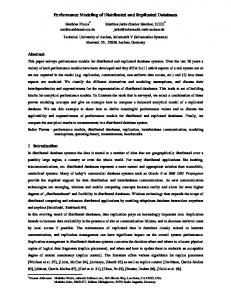
IV. N UMERICAL R ESULTS AND D ISCUSSIONS In order to verify our analysis, we built a simulation model in MATLAB, in which one slot corresponds to 1 msec. We run each simulation for 150000 slots and time-average the results. Unless otherwise stated, L = 20, τ = 50 and unlimited RL are set. At the beginning of a simulation we randomly distributed M terminals over the NRES2 -, the NRES3 -, and the CON states for 0 ≤  ≤ U . The parameters of VoIP traffic are given in Section II-B. Note that VoIP capacity for SPS with initial random access is defined as the maximum of admitted terminals M without exceeding a predefined packet dropping rate. In the following examples, we consider one PRACH in a slot, which takes six radio RBs. Note that 18 terminals can typically use one PUCCH of one radio RB in SPS with SRI. Thus, 108 terminals can be supported by six RBs in SPS with SRI. We first examine the effect of random access in SPS with respect to stability and the backoff algorithm, which provides the feasibility of SPS with initial random access. In addition, we compare our system with PRMA and then present the effect of K on the performance. Bistability: We examine bistability of this system, by solving (30) for the equilibrium points. We denote the PMFs of c0 and c in the system by πc0 for 0 ≤ c0 ≤ M , which is obtained by simulations. In Fig. 3 we depict respectively F (c0 ) and two examples of πc0 for P = 2, D = 5, U = 10, K = 2, M = 100 and L = 20 obtained from two simulation runs. As F (c0 ) shows three roots of (30), we can observe two different distributions of πc0 , which implies bistability. As previously mentioned, in this case we can obtain the system performances at locally stable equilibrium points for some finite time period in a simulation. To mitigate such a bistability, we consider three schemes. First, we apply a retry limit RL in simulations, which limits the number of retransmissions. If the number of retransmissions exceeds RL , the terminal drops the packet and gets back to the NRES2 state. We denote by Pr the probability

4454

IEEE TRANSACTIONS ON WIRELESS COMMUNICATIONS, VOL. 11, NO. 12, DECEMBER 2012

TABLE II S TABILIZED SYSTEM PERFORMANCE WITH VARIOUS PARAMETERS RL = 5, U = 10 P = 2, K = 2 1.38 6.92 0.24 0.50

2 3 Packet dropping rate (%)

Throughput of traffic channel, ζd (packets/slot)

ζd (packets/slot) d (slots) Pd × 100(%) Pr × 100(%)

1.5

1

0.5

U U U U U U U U U

0 70

= 10, τ = 50 (ana) = 10, τ = 40 (ana) = 5, τ = 50 (ana) = 15, τ = 50 (ana) = 10, τ = 40 (sim) = 10, τ = 50 (sim) = 5, τ = 50 (sim) = 15, τ = 50 (sim) = 10, P = 64 (sim) 80

90 100 110 120 Number of terminals, M

130

1.5 1

0 70

80

90 100 110 120 Number of terminals, M

130

The effect of U on the system performance.

PRMA (ana) PRMA (sim)

Packet dropping rate (%)

2

= 10, τ = 40 (ana) = 10, τ = 50 (ana) = 5, τ = 50 (ana) = 15, τ = 50 (ana) = 10, τ = 40 (sim) = 10, τ = 50 (sim) = 5, τ = 50 (sim) = 15, τ = 50 (sim) = 10, P = 64 (sim)

(b) Packet dropping rate.

2

P = D = 2 (ana)

1.5

P = D = 2 (sim)

1

0.5

0

10

20

30

40

50

Number of terminals, M Fig. 5.

2.5

U U U U U U U U U

RL = ∞, U = 10 P = 5, K = 2 1.41 (Ana: 1.44) 6.45 (Ana: 6.25) 0.11 (Ana: 0.1) 0

0.5

(a) Throughput of traffic channels. Fig. 4.

RL = ∞, U = 15 P = 2, K = 2 1.38 (Ana: 1.43) 9.87 (Ana: 9.5) 0.9 (Ana: 0.7) 0

Comparison of PRMA and SPS with random access

that a packet is dropped due to this retry limit, which is given in the first column of Table II. Secondly we control U , and thirdly increase P . The corresponding results are given in the second and third columns of Table II. While increasing U or reducing RL also stabilize the system by dropping the packet forcibly, Pd and/or Pr would be sacrificed. Therefore we can conclude that increasing P from 2 to 5 is the most effective way to mitigate instability, by relieving congestion

in the random access channel3 . Thus, a sufficient number of RAPs should be secured according to the maximum number of VoIP users to be admitted, and then RL can be further applied to prevent bistability. On the other hand, a large U might not be desirable for delay-constrained applications, since it causes large random access delays. Note that the system shown in Fig. 3 is bistable with 100 terminals. However, as shown in the second and third columns of Table II, 100 terminals can be supported with τ = 50 and 1% packet dropping rate in the two stabilized systems with U = 15, or with P = 5. The effect of window size U : With P = D = 5 and K = 1 we vary U from 5 to 15 and use τ = 40 and 50 in Figs. 4(a)4(b). Fig. 4(a) depicts ζd , while the packet dropping rate is presented in Fig. 4(b). A smaller U (faster access) provides much lower Pd , while ζd is insensitive to U except at U = 5 and M = 115 (i.e., when the system is highly congested). U = 5 causes the instability of the system around M = 115 due to more frequent retransmissions that lead to congestion in the random access channels. To determine the VoIP capacity with τ = 50, we can observe that 130 terminals is maximally accepted by U = 15, while U = 10 can accept more than 130 VoIP terminals. We also observe Pd with a smaller τ = 40 (slots), i.e., a tighter delay constraint, which shows a higher Pd and hence a lower quality of VoIP traffic. Although some simplifications have been made in our model, we can see that 70 terminals can be admitted. In addition, we simulate the system with P = 64, τ = 50, U = 10. We present simulation result only for this system due 3 Note that we can approximately have ζ = P e−1 (packets/slot) as the a maximum throughput of the random access channel for the system with P RAPs, which gives ζa = 0.735 for P = 2 and ζa = 1.839 for P = 5, respectively.

0.8

1.8 1.6 K K K K K K K K

1.4 1.2 1

0.8 70

80

90

100

=1 =2 =4 =8 =1 =2 =4 =8

110

(ana) (ana) (ana) (ana) (sim) (sim) (sim) (sim)

120

9 8.5 8

130

0.5 0.4

(ana) (ana) (ana) (ana) (sim) (sim) (sim) (sim)

0.3 0.2

70

80

90

100

110

120

Number of terminals, M

(a) Throughput of traffic channels.

(b) Packet dropping rate.

0.1 K K K K K K K K

=1 =2 =4 =8 =1 =2 =4 =8

(ana) (ana) (ana) (ana) (sim) (sim) (sim) (sim)

7.5 7 6.5 6 70

0.6

=1 =2 =4 =8 =1 =2 =4 =8

Number of terminals, M

Probability mass function of W

Random access delay, d (slots)

9.5

0.7

K K K K K K K K

0.1

10

Fig. 6.

4455

2

Packet dropping rate (%)

Throughput of traffic channel, ζd (packets/slot)

SEO and LEUNG: PERFORMANCE MODELING AND STABILITY OF SEMI-PERSISTENT SCHEDULING WITH INITIAL RANDOM ACCESS IN LTE

80

90

100

110

120

130

K K K K K

0.08

= 1, M = 8, M = 1, M = 8, M = 8, M

= 115 = 115 = 115 = 115 = 125

20

25

130

(ana) (ana) (sim) (sim) (sim)

0.06

0.04

0.02

0 0

5

10

15

Number of terminals, M

Random access time, W

(c) Mean random access delay.

(d) PMF of random access times.

30

The effect of K on the system performance.

to computational complexity in (15) for such large P . Even though the packet dropping rate in the system with P = 64 and U = 10 is improved compared to the system with P = 5 and U = 10 (the same backoff window size), it is noticeable that the system with P = 5 and U = 5 shows compatible low packet dropping rate until M = 115. This implies that, rather than just increasing P , more dynamic control of U can lead to large improvements of the packet dropping performance. An optimal way of controlling U is to adjust the expected value of U , i.e., E[U ], to total number of backlogged terminals, c. We then have c/E[U ] = c0 = P (refer to (32)), which requires the backlog size estimation. Comparison with PRMA: In Fig. 5, we compare the packet dropping rate, i.e., Pd × 100 (%), of SPS with random access (P = D = 2) against that of PRMA with U = 5 and K = 1. While the original PRMA [11] uses a permission probability as the backoff algorithm, the PRMA presented in Fig. 5 has been modified to use the UB algorithm for a fair comparison. As expected, the VoIP capacity in SPS with random access is almost doubled under a 1% packet dropping rate due to increased P and D. The discrepancies between analysis and simulation at M = 26 in PRMA and M = 50 in SPS with random access can be explained by the fact that the systems have multiple equilibrium points with

these population sizes. Thus, the simulation results are timeaveraged values in bistable systems. While the VoIP capacity of PRMA depends only on a single parameter (permission probability in [11] or U here), that of SPS with random access depends on the parameters U , P , D and K. The effect of K: Recall that K is used for detecting silence periods. We examine the effects of K on the system performance with U = 10, and P = D = 5 in Figs. 6(a)-6(d). In Fig. 6(a) we can observe that ζd slightly decreases due to longer holding times of traffic channels as K increases. While ζd shows good agreements between analysis and simulation results, this is not the case with the packet dropping rate and d, particularly for larger M and K in Figs. 6(b) and 6(c). Although the systems with those parameters are stable, EPA cannot evaluate system performance reliably. This is possibly caused by two reasons. First, by examining the PMF of the random access time, W , for M = 115 and M = 125 in Fig. 6(d), we can see that analysis and simulation results show some agreement for K = 1, while high fluctuations and disagreements are found either for K = 8 or for M = 125. When we increase K, the number of backlogged terminals decreases to as small as c∗0 < 0.1 in analysis and simulation. Although the difference of c∗0 between analysis and simulation (slightly underestimated by analysis) is quite small, the per-

4456

IEEE TRANSACTIONS ON WIRELESS COMMUNICATIONS, VOL. 11, NO. 12, DECEMBER 2012

centage of such differences is no longer negligible. In these cases, simulation results show a longer tail distribution of W than analytical results, which might cause mismatch between analytical and simulation results in Fig. 6(b). Secondly, even for a stable system, if the distribution of πc0 (or πc ) is asymmetric, then it might result in a mismatch between analysis and simulation results because c∗0 in (30) represents only an averaged value for the equilibrium condition. In order to find K properly, we suggest the following cost function: maximize γ1 ζd (K) − γ2 Pd (K, τ ) K

(42)

where γ1 and γ2 are weighting factors, and ζd is the normalized traffic channel throughput, i.e., ζd (K) = ζd (K)/D. Note that γ1 and γ2 can be determined based on QoS requirements of a traffic. For VoIP traffic, we can have γ1 < γ2 . In this example, K = 2 might be favourable, because ζd gets lower with larger K. V. C ONCLUSION In this paper we have examined the feasibility of SPS with initial random access for VoIP traffic in LTE by constructing an approximate model based on EPA to analyse its performance. In particular we have shown the VoIP capacity as the number of VoIP terminals that can be accommodated without exceeding some packet dropping probability, when initial random access is used. From our study, it can be conjectured that SPS with initial random access might be alternatively used or provide additional VoIP capacity improvement, if the cost of PUCCH for SRI not used in the OFF period of an application would be expensive. We have also investigated the effect of K, the number of empty transmission slots before the reserved traffic channel is released, and the effect of U on VoIP capacity. Although our analytical model cannot provide reliable performance evaluations for large K, VoIP capacity has been estimated with various U and K = 1. We have shown also the instability of SPS with random access based on UB algorithm (without retry limit), and discussed how to stabilize the system. We can conclude that, while a retry limit can effectively stabilize the system at the expense of a reasonable Pr , optimal control on U would be more desirable. ACKNOWLEDGEMENT The authors would like to thank Ki-Dong Lee for constructive comments on this paper. R EFERENCES [1] H. Holma and A. Toskala, LTE for UMTS: OFDMA and SC-FDMA Based Radio Access. John Wiley & Sons Ltd., 2009. [2] Third Generation Partnership Project; Evolved Universal Terrestrial Radio Access (E-UTRA) Medium Access Control (MAC) protocol specification, 3GPP TS 36.321 V.9.1.0 (2009-12). [3] M. Rinne, M. Kuusela, E. Tuomaala, P. Kinnunen, I. Kovacs, and K. Pajukoski, “A performance summary of the evolved 3G (E-UTRA) for voice over Internet and best effort traffic,” IEEE Trans. Veh. Technol., vol. 58, no. 7, pp. 3661–3673, Sep. 2009. [4] Q. Bi, S. Vitebsky, Y. Yang, Y. Yuan, and Q. Zhang, “Performance and capacity of cellular OFDMA systems with voice-over-IP traffic,” IEEE Trans. Veh. Technol., vol. 57, no. 6, pp. 3641–3652, Nov. 2008.

[5] H. Lee, T. Kwon, and D.-H. Cho, “An enhanced uplink scheduling algorithm based on voice activity for VoIP services in IEEE 802.16d/e system,” IEEE Commun. Lett., vol. 9, no. 8, pp. 691–693, Aug. 2005. [6] H. Lee, H.-D. Kim, and D.-H. Cho, “Smart resource allocation algorithm considering voice activity for VoIP services in mobile-WiMAX system,” IEEE Trans. Wireless Commun., vol. 8, no. 9, pp. 4688–4697, Sep. 2009. [7] S.-M. Oh, S. Cho, J.-H. Kim, and J. Kwun, “VoIP scheduling algorithm for AMR speech codec in IEEE 802.16e/m system,” IEEE Commun. Lett., vol. 12, no. 5, pp. 374–376, May 2008. [8] S. Tasaka, Performance Analysis of Multiple Access Protocols. MIT Press, 1986. [9] Third Generation Partnership Project; Evolved Universal Terrestrial Radio Access (E-UTRA) Physical layer procedure, 3GPP TS 36.213 V.9.2.0 (2010-06). [10] C.-H. Ng, L. Yuan, W. Fu, and L. Zhang, “Methodology for traffic modeling using two-state Markov modulated Bernoulli process,” Computer Commun., vol. 22, no. 13, pp. 1266–1273, Aug. 1999. [11] S. Nanda, D. J. Goodman, and U. Timor, “Performance of PRMA: a packet voice protocol for cellular systems,” IEEE Trans. Veh. Technol., vol. 40, no. 3, pp. 584–598, Aug. 1991. [12] S. Nanda, “Stability evaluation and design of the PRMA joint voice data system,” IEEE Trans. Commun., vol. 42, no. 5, pp. 2092–2104, May 1994. [13] Z. Zhang and Y.-J. Liu, “Comments on ‘The effect of capture on performance on multichannel slotted ALOHA system’,” IEEE Trans. Commun., vol. 41, no. 10, pp. 1433–1435, Oct 1993. [14] S. Tasaka, “Stability and performance of the R-ALOHA packet broadcast system,” IEEE Trans. Computers, vol. C-32, no. 8, pp. 717–726, Aug. 1983. [15] L. Kleinrock and S. S. Lam, “Packet switching in a multiaccess broadcast channel: performance evaluation,” IEEE Trans. Commun., vol. COM-23, no. 4, pp. 410–423, Apr. 1975. [16] H. Qi and R. Wyrwas, “Markov analysis for PRMA performance study,” in Proc. 1994 IEEE Vehicular Tech. Conf., vol. 2, pp. 1184–1188. [17] L. Kleinrock, Queueing Systems: Volume I–Theory. Wiley Interscience, 1975. Jun-Bae Seo (S’08-M’12) received B.S., M.Sc. degrees in Electrical Engineering from Korea University, 2000 and 2003, and received the Ph.D. degree from the University of British Columbia (UBC), Vancouver, Canada in 2012. He was the recipient of a Natural Sciences and Engineering Research Council Postgraduate Scholarship from September 2009 to August 2011. From 2003 to 2006, he was with Electronics and Telecommunications Research Institute (ETRI), Korea, as a member of the engineering staff, carrying out research on IEEE 802.16 systems. He is now a Posdoctoral Research Fellow with UBC. Victor C. M. Leung (S’75-M’89-SM’97-F’03) is a Professor and holder of the TELUS Mobility Research Chair in Advanced Telecommunications Engineering in the Department of Electrical and Computer Engineering at the University of British Columbia in Vancouver, Canada, where he earned the B.A.Sc. and Ph.D. degrees in 1977 and 1981, respectively. His research interests are in the broad areas of wireless networks and mobile systems, in which he has co-authored more than 600 technical papers in international journals and conference proceedings. Several papers co-authored by him and his students have won best paper awards. Dr. Leung is a registered professional engineer in the Province of British Columbia, Canada. He is a Fellow of IEEE, the Engineering Institute of Canada, and the Canadian Academy of Engineering. He has served on the editorial boards of the IEEE Journal on Selected Areas in Communications, IEEE Transactions on Wireless Communications and IEEE Transactions on Vehicular Technology, and is serving on the editorial boards of the IEEE Transactions on Computers, IEEE Wireless Communications Letters, Journal of Communications and Networks, Computer Communications, as well as several other journals. He has guest-edited many journal special issues, and served on the technical program committees of numerous international conferences. He has contributed to the organization of many conferences and workshops. He was a winner of the 2011 UBC Killam Research Prize and the IEEE Vancouver Section Centennial Award.