Performance Modeling of Distributed Collaboration Services Toqeer Israr
Gregor v. Bochmann
School of Information Technology and Engineering (SITE)
School of Information Technology and Engineering (SITE)
University of Ottawa
University of Ottawa
800 King Edward Avenue, Ottawa, Ontario, Canada, K1N 6N5
800 King Edward Avenue, Ottawa, Ontario, Canada, K1N 6N5
1-613-562 5800 x 6433
1-613-562 5800 x 6205
[email protected]
[email protected]
ABSTRACT This paper deals with performance modeling of distributed applications, service compositions and workflow systems. From the functional perspective, the distributed application is modeled as a collaboration involving several roles, and its behavior is defined in terms of a composition from several sub-collaborations using the standard sequencing operators found in UML Activity Diagrams and similar formalisms. For the performance perspective, each collaboration is characterized by a certain number of independent input events and dependent output events, and the performance of the collaboration is defined by the minimum delays that apply for a given output event in respect to each input event on which it depends. We use a partial order to model these delays. The paper explains how these minimum delays can be measured through testing. It also provides general formulas by which the performance of a composed collaboration can be calculated from the performance of its constituent subcollaborations and the control structure which determines the order of execution of these sub-collaborations. Proofs of correctness for these formulas a given and a simple example is discussed throughout the paper.
Categories and Subject Descriptors D.2.8[Software Engineering]: Metrics - Performance measures
General Terms Algorithms, Measurement, Performance, Verification.
Keywords performance modeling, software performance, partial order, collaborations, UML activity diagrams, distributed applications, web services
1. INTRODUCTION Various kinds of models are used for a system design and development process. Amongst several notations, some are UML Activity Diagram[15], Use Case Maps (UCM)[5], the Process Definition Language(XPDL), Business Process Execution Language (BPEL), Web Services Choreography Description Language (WS-CDL) [19] and Petri Nets. All these mentioned
notations can potentially be decomposed into sub activities and further into sub-sub-activities. Most of these notations, though, assume the basic activities in the decomposition to be allocated to a single system component. However, most of the applications have activities which are modeling collaborations between several system components, for instance an interaction between a client and a server. To this end, a modeling paradigm based on collaborations has been proposed [1] which can be represented through a combination of UML Collaboration diagrams and a partially ordered set of input and outputs.
While the realization of distributed designs for such collaboration services often pose tricky questions for the correctness of the required communication protocols in terms of the messages being exchanged between the different system components participating in the realization of the distributed service (see for instance [1] and [6]), we concentrate in this paper on the performance aspects of such collaborations. We use the concept of partial orders to model the temporal relationships between the different subactivities within a collaboration, and use ideas from the PERT (Project Evaluation and Review Technique) technique [8] commonly used for project management. We also build on a testing technique developed for systems that implements a behavior defined in terms of a partial order relationship between input events and output events [4], and show how a similar technique can be applied for performance analysis of distributed applications. We base our analysis on the collaboration roles involved and we make the assumption that each role can be implemented by a multi-threaded component.
The paper is structured as follows. In Section 2, we review the modeling paradigm based on collaborations and introduce an example. This section also describes the rules that underlie the concepts of strong and weak sequencing. In Section 3, we discuss how such system models can be modeled using partial orders. In Section 4, we introduce performance considerations, mainly related to the delays implied by the execution of the different subactivities within collaborations. A general timing constraint is established which determines the earliest time that a given output event of a collaboration can be produced. Inspired by the testing
procedure of [4], we will also show how the parameters determining the performance of a collaboration can be measured. In Section 5, we propose and prove formulas to calculate the performance of composite collaborations, and applied to a simplified version of the running example introduced earlier.
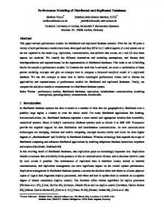
and after that, the dispatcher ends the shift. Meanwhile, the cab takes the client to the destination and is paid for the services rendered, upon which the sequence for the cab and for the client then ends. This system can accept new clients and drivers, which would be serviced as long as the dispatcher continues to loop and execute.
2. MODELING DISTRIBUTED COLLABORATION SERVICES: AN EXAMPLES An example of Cab Dispatcher System (CDS) is presented in Figure 1.0a. It consists of 5 sub-collaborations and 3 roles – client, dispatcher and cab. For each of these roles there will exist an input event (client requesting cab, dispatcher being available, and cab being available) and three output events (client reaches their destination and makes payment to driver, cab signs off, and dispatcher signs off). These input and output events are initiating and terminating events, respectively of this CabDispatcher collaboration. Initiating event[1] represents the starting of an action in the collaboration, for which there are no other actions in that collaboration that precedes that action. Similarly the terminating event [1] represents the end of an action in a collaboration, for which there is no other action in a collaboration that succeeds this action in that flow of execution.
These initiating and terminating events should not be confused with the starting and the ending events. The starting event represents the starting of the actions in a collaboration for a single component, for which there are no other actions in that collaboration for that component that precede that action. Similarly, an ending event represents the end of an action in a collaboration for a single component, for which there are no other actions in a collaboration for that component, that succeed that action. A starting event can be an initiating event but does not have to be whilst an initiating event has to be one of the starting events. Similarly, an ending event can be a terminating event but does not have to be whilst a terminating event has to be one of the ending events.
In order to define the behaviour of a collaboration, we use Bochmann’s [1] diagram notation, based on most of UML Activity Diagram constructs as shown in Figure 1.0a. For each of these sub-collaborations, initiating and starting events are represented by dark dots “●” while ending and terminating events are represented by vertical bars “|”. More discussion on events will follow in context of partial ordering. We also note that initial node not only models the start of all the flows in a collaboration, but also represents the starting of all the roles involved.
We consider the example of cab dispatcher system. The client (Cl) requests a cab from the dispatcher (Di). The cab, when available, comes in and the dispatcher adds the cab to the queue of available cabs. The dispatcher also concurrently services the client’s requests. The client, whilst waiting for the cab has the option to cancel the cab. Once there is a cab in the queue, the dispatcher assigns the cab to the client and goes back and waits for more cabs and clients. The dispatcher does this for n times
Cl
R: Request Cab
I: Initialize & add to Q
Di
D i
Cab
w w
w
Di Cl
C: Cancel
Di
A: w Assign Cab
Cab
w Cl
m: Meet & Drive
Cab
Figure 1.0a – Collaboration of Cab Dispatcher System
2.1 Strong and Weak Sequencing Between the sub-collaborations in Figure 1.0a, there is a choice of weak and strong sequence operators [1] to be used. Two collaborations C1 and C2 are said to be strongly sequenced when all the sub-collaborations of C1 are be completed before any subactivity of C2 starts. However, weak sequencing between C1 and C2 means that each role locally applies sequencing to the local sub-collaborations of C1 and C2, that is, a role may start with sub-collaborations that belong to C2 as soon as it has completed all its local sub-collaborations that are part of C1. Strong sequencing implies weak sequencing, but not inversely. In weak sequencing, if a role is not involved in C1, it may start with subcollaborations of C2 even before C1 begins its execution.
In our example of Figure 1.0b and 1.0c, let us consider 2 collaborations – S1: Send Info followed by S2: Send Info. Send Info in both collaborations has the exact same behaviour – R1 sends a message to R2, and based on that message, R2 does some processing and then terminates.
If we consider strong sequencing, as shown by the label “s” on sequencing arc in Figure 1.0b, then all the terminating events(belonging to only R2), completes its processing in S1:Send Info, before the initiating events of S2:Send Info can occur. This would mean the R2 has to complete its processing in S1:Send Info before R1 in S2: Send Info may start. Also note, the time of the initiating event of S2: Send Info is the time when all of the terminating events occur (in this case, there is only 1 terminating event).
R1
S1: Send Info
R2
of a role has to occur after the input of the same role in the same collaboration. 3 input events
3 input events CI1
w R1
S2: Send Info
S1: Send Info
S2: Send Info
CI1
CI2
CI3
CO1’
CO2’
CO1’
CO3’
3 output events
CO2’
CO3’
3 output events
Figure 3.0a – The POS corresponding to a simple collaboration
R2
s R1
CI3
C
R2
Figure 1.0b – Weak Sequencing
R1
CI2
R2
Figure 1.0c – Strong Sequencing Now, let us consider weak sequencing between “S1: Send Info” and “S2: Send Info”(as shown by “w” on the sequencing arc of Figure 1.0c). This implies the actions of each role of “S2: SendInfo” may start as soon as those roles have completed their actions belonging to the previous collaboration, in this case “S1: Send Info”. Hence, as soon as the R1 sends the message to R2 in S1:Send Info, R1 can start sending a message for S2:Send Info. The important thing is that R1 need not to wait for R2 to complete its execution of S1:Send Info before R1 starts its execution in S2: Send Info.
3. DESCRIBING COLLABORATIONS WITH PARTIAL ORDERS 3.1 Review of Partial Orders Inspired by Partial Order Input Output Automata (POIOA) [4], an extension of Input Output Automata, we introduce Partial Order Systems (POS). In a POS, each collaboration has a set of independent initiating events. These initiating events trigger the execution of some internal actions resulting in a set of output events. Figure 3.0a shows a POS corresponding to a simple collaboration involving three independent inputs and three outputs. The outputs are not ordered relative to one another directly but each output has a dependency on the inputs as indicated by the arrows, “Æ”. For instance, event CO1’ can only occur after the occurrence of event CI1, but for event CO2’ to occur, both (CI1 and CI2) must occur first. We can write this as (CI1 ÆCO1’), (CI1 Æ CO2’) and (CI2 Æ CO2’)).
Having an operator to model alternatives is a very common and a useful concept in UML. However, we had to improvise as Partial Ordering does not allow modeling of alternative paths. Inspired by the choice symbol in UCM[5], we introduce a new symbol in Partial Ordering to represent a choice in a system. As can be seen in Figure 3.0b, it is a rectangular box with multiple branches stemming out, with each branch having an event associated with it. This will be illustrated with an example later on. I1 or
I1 I2
I3
I2
I3
Figure 3.0b – Choice representation in POS
3.2 Modeling with Partial orders In this section, we would like to discuss the POS resulting from a given collaboration. For a given collaboration, each initiating and starting event translates into an input event of a POS, and each terminating and ending event translates into an output event of a POS.
Figure 4.0a shows a POS corresponding to Assign Cab subcollaboration, from Figure 1.0a, involving 1 initiating event (initiated by dispatcher), 1 starting event for driver, and 2 terminating events, cab getting assigned and dispatcher updating the cab available queue. Direct and derived dependencies are shown using the solid and the dashed arcs respectively. Dispatcher AI1
Driver AI2
Assign Cab
There also exists a set of derived dependency amongst the inputs and the outputs relative to each other also, shown by the dashed arrow in Figure 3.0a. One such dependency is event CO3’ occurs after CI2. Since (CI2 Æ CI3) and (CI3 Æ CO3’), then it is intuitive to derive (CI2 Æ CO3’). Other derived dependencies can also be derived due to local ordering, where the output event
AO1’
AO2’
Figure 4.0a – POS of the Assign Cab sub-collaboration
3.2.1 Modeling Weak and Strong Sequencing with Partial orders As discussed before, there could be strong and weak sequencing between any two collaborations. In Figure 1.0a, AssignCab is weakly sequenced with Meet&Drive, which is abstracted by ClientServing in Fig 4.0b. This to help us realize when each role becomes available, before and after the weak sequenced operation. Client
Dispatcher
CI1
Cab
CI2
CI3
AI1
AI2
Assign Cab Client Serving
AO2’
AO1’
MI1
MI2 Meet & Drive MO2’
MO1’
CO1
CO2
CO3
Figure 4.0 b – POS of 2 weakly sequence collaborations In ClientServing, local ordering applies for the starting and initiating events of AssignCab. This means as soon as there are inputs available for Cab and Dispatcher, they are passed onto AssignCab. Since Client is involved only in Meet&Drive, client may potentially start Meet&Drive as soon as there is an input for Client at ClientServing. Client
Dispatcher
CI1
CI2
Since AssignCab and Meet&Drive are weakly sequenced, local ordering applies amongst the roles involved. Hence, the cab can start as soon as it completes AssignCab. Since dispatcher is not involved in Meet&Drive, it does not wait for Meet&Drive to be completed and it can start its next collaboration after ClientServing. The client could have potentially started Meet&Drive before the completion of AssignCab, but it would not have been able to since cab is the only initiating role in Meet&Drive and hence client has to wait for the cab to start Meet&Drive before it starts to execute.
In Figure 4.0 c, we model the same two sub-collaborations as we did Figure in 4.0b, but now we assume they are strongly sequenced. As discussed before, this means that all the initiating events in Meet&Drive will occur only and only once all the terminating events of the previous collaboration, AssignCab, have occurred. We call this event Final Action event – when all the terminating events have occurred, denoted by AOF (Final Output of sub-collaboration AssignCab). This also gives us the time of the initiating events for the next collaboration, Meet&Drive, which is the same time as of the Final Action of the previous collaboration, AssignCab.
3.2.2 Modeling Cab Dispatcher System with Partial orders In Figure 4.0d, we model the Cab Dispatcher System of Figure 1.0a as a Partially Ordered System, where the dependencies are again shown by arrowheads. In Figure 1.0a, we can see that there are three roles involved, driver, dispatcher and the client, and hence 3 initiating events, namely I1, I2, and I3 are shown in Figure 4.0d. Input I1 leads to RI1 and I3 leads to II2, which are both a simple of case of initiating the RequestCab and Initiatlize&AddtoQ collaboration. Client
Cab CI3
AI1
I1 RI2
RI1
AI2
I4
O1
I3 II1
or
RO1’ CI1
RO2’
IO1’ AI1
CO1’ AO1’
AOF
MI1 Meet & Drive
IO2’
CI2
AO2’
MI2
II2 Initialize & Add to Q
Cancel
MI1
Driver
Request Cab Assign Cab
AO1’
Dispatcher I2 or
back to I2
AI2 Assign Cab AO2’ MI2 Meet & Drive
MO1’
MO2’
MO2’
MO1’
Figure 4.0 d – POS of the detail collaboration ProcessOrder CO1
CO2
CO3
Figure 4.0 c – POS of 2 strongly sequence collaborations
POS of RequestCab sub-collaboration has only one initiating event RI1, one starting event RI2, one terminating event RO1’ and one ending event RO2’. Hence, we can see there are
dependencies between the two inputs, RI1 and RI2. The output event RO1’ will happen only after RI1 due to local ordering and same is true for RO2 and RO2’.
POS of other sub-collaborations follow as described above, where the ordering relationships are realized using the event types (initiating, starting, ending, terminating), weak and strong sequencing and local ordering relationships.
4. PERFORMANCE CHARACTERISTICS OF PARTIAL ORDER SPECIFICATIONS 4.1 Direct & Indirect Dependency Amongst Execution Threads in a Single Activity It is quite common to have concurrent input events for a single collaboration. Sometimes there are direct dependencies amongst these events which are straightforward to realize while other time there are indirect dependencies.
Direct dependency is when an event is waiting on the occurrences for one (or more) other events. For example, in Figure 5.0, o2 is directly dependent on inputs i1 and i2.
i1
4.3 Deriving Performance Parameters using Test Suite
We are interested in Minimum Execution Time Delay, de1e2 and the ordering relationship between the initiating and the output events. Bochmann et al., in [4] discuss an approach for testing systems specified as Partial Order Input/Output Automata (POIOA). They propose a testing methodology for systems specified as POIOA, and compare it with the case of traditional asynchronous I/O automata. Using their model and methodology, they reduce the complexity in testing as well as reduce the number of tests required for testing transitions with concurrent inputs.
i2
A o1
dependency exists between events e1 and e2, that dependency is written as oe1e2 and the corresponding delay between e1 and e2 would be Δde1e2. oe1e2 means that e2 succeeds e1 and de1e2 is the time difference between the event e1 and e2, also known as Execution Time Delay. A time delay between 2 events, e1 and e2, where there is no delay due to any dependencies from any other events other than e1, is called Minimum Execution Time Delay (METD), denoted by Δ e1e2. We write t e for the time instant when event e occurs. For a given collaboration, we write I for the set of input events and O for the set of output events. For an input ix ε I, we write EB(ix) = { iy ε I, iy ≠ ix } meaning “Every Input But” ix.
o2
Figure 5.0 – Collaboration with Dependent & Independent Execution Threads However, indirect dependency is when an event, e1, does not directly affect another event, e2, but could rather trigger some actions internally, which would have some effects on e2. This is usually the case when there are some shared resources being accessed by multiple threads of control. For example, in Figure 5.0, o1 is only directly dependent on only i1 and not on i2 or o2. However, now let us assume that during the execution of i1 and i2, both access the same database. One scenario can arise where one thread has a lock on the database, which in effect, makes the other thread wait for the database longer than without the lock. This sort of dependency will be called indirect dependency as one execution thread is affecting the execution time of the other thread indirectly.
For this paper, we only consider direct dependencies and assume that there are no indirect dependencies among different events.
4.2 Adding Performance Parameters to Partial Orders As discussed, a collaboration can be represented as a set of partially ordered input and output events. We propose if a
We adapt their testing methodology for our needs. For their testing methodology, the authors assume the input events of a given collaboration could be dependent on the output events of the same collaboration. In our POS, we restrict this kind of dependency and do not allow the input events to be dependent on the output events of the same collaboration. We adapt their testing methodology to realize the ordering relationship between the initiating and the output events and measure the Minimum Execution Time Delay between these events as follows. For each input event ix ε I, the following test suite should be executed: Step 1. Allow all the input events in EB(ix) to occur and allow their resultant actions to be executed to the fullest. This could result in a set of some output events, which we call S1ix. Step 2. Now allow the input event ix to occur and allow the resulting actions to be executed to the fullest. Observe the set S2ix of output events produced from this execution. Measurement of time between output om ε S2ix and the input ix will yield Minimum Execution Time Delay, dixom. Since the production of event om ε S2ix was due to the input event ix, this clearly shows there is a dependency of each output event in set S2ix on ix. Continuing with further analysis, we can see that once step 1 and step 2 are repeated for all x in collaboration C, we should then examine each of the output events in the sets S2ix. An output
event om is dependent on all of the input event ix which produced the set S2ix, that contains the event om {om ε S2ix, om ε S2iy, x≠y, then om is dependent on both ix and iy}. In Step 2, the Minimum Execution Time Delay, Δixom, is measured also between an input event ix ε I and the output event om ε S2ix. This time delay does not include time for any waiting due to any dependencies or such since all the remaining events and their relating primitive actions have already been allowed to execute to their fullest in Step 1. The nature of the partial order imposes that the earliest time that an output event O can be executed is at a time t O that satisfies for all input events, I, for which there is a oIO that exist in the partial order: t I + ΔIO ≤ t O. Event O can be dependent on multiple input events. Event O can not occur until executions from all of these events are completed and then and only then can event O can occur. This means that the earliest possible execution time for event O is:
To calculate the time of the output event, we rewrite (Earliest Time) formula as: tCOt = max x=1…k (tCIx + ΔCIxCOt),
(1)
where there are k inputs which have a dependency on output event Ot We propose (1) can be applied to any of the above sequencing operators but each with its own definition of ΔCIjCOt. In the next section, we propose and provide proofs for the various definition of Minimum Execution Time Delay ΔCIjCOt for collaborations composed by the above discussed sequencing operators.
5.1 Strong Sequence Figure 6.0 shows strong sequencing between two collaborations A and B. As discussed already, we use Final Action event to represent the event when all the terminating events have occurred in A as shown in Figure 6.0.
where the maximum is taken over all input events I on which event O depends on
Proposition 1.0: As shown in Figure 6.0a, if two collaborations, collaboration A with k inputs and k’ outputs and collaboration B with m inputs and m’ outputs, are strongly sequenced, then the time of the output is:
5. DERIVING GENERAL FORMULAS FOR STANDARD SEQUENCING OPERATORS
tCOt = max x=1…k (tAIx + maxy=1..k’(ΔAIxAOj)
tO = max I (t I + ΔIO),
(Earliest Time)
Bochmann and his group in [1], has developed and implemented a methodology to derive component designs from global service and workflow specifications based on the more common sequencing operators described in UML Activity Diagrams and High-Level MSCs such as weak sequence, strong sequence, weak while loop, strong while loop, and choice. They illustrate this with an example of a telemedicine consultation service involving multiple roles. For this global specification, they use their transformation rules based on the sequencing operators to derive each of the role’s behaviour. We derive the performance of the global collaboration based on the performance of each sub-collaboration. We model the subcollaborations with the above defined notations, and represent them as partial orders. We wish to derive the general performance formulas which we can apply to the sequencing operators of sub-collaborations to yield the performance metrics of the global collaboration. We already have analyzed and calculated the time instant of the output events produced relative to the input events which these output events depend on and produced the well-defined formula (Earliest Time). We seek the time instant of the output event (tCO) for a composed collaboration C, provided it has some j input events. Collaboration C is an abstraction of collaboration A and collaboration B with the above discussed sequential operators.
BIs
+ maxs=1..m(Δ AI1
(2)
BOt)),
AIk
A AO1
CI1
AOk'
CIk
C
AOF
CO1’ BI1
COm’
BIm
B BO1
BOm'
Figure 6.0a – POS equivalent
Figure 6.0b - abstraction
Proof: tAOF is by definition the maximum of tAOj for ∀ j inputs: tAOF = maxy=1..k’(tAOy), where there are k inputs and k’ outputs for A
(3)
From (1), we already know the time instant of the output events for collaboration A: tAOy = maxx=1..k (tAIx + ΔAIxAOj) (4) Using this definition of the time of the output for A (4) in (3), we get: tAOF = maxy=1..k’(maxx=1..k(tAIx + ΔAIxAOy)) (5) We can rewrite (5) as: tAOF = maxx=1..k (tAIx + maxy=1..k’(ΔAIxAOy))
(6)
The time instant for the output event of collaboration B is defined (similar to A’s) as: tBOt = tCOt = max s=1..m (tBIs + ΔBIsBOt) (7) where there are m inputs and m’ outputs for B To calculate the fastest execution, we consider time of the initiating events of collaboration B is the same as the time for the final action event of collaboration A, therefore: tBIs = tAOF for s = 1…m (8) Knowing (8), we can use (6) in (7): tCOt = max s=1..m (maxx=1..k (tAIx + maxy=1..k’(ΔAIxAOy)) + ΔBIsBOt)
maxs=1..m (ΔBIsBOt))
A CI1
CIk
C B BO1
CO1’
COm’
BOm'
Figure 7.0 a – POS equivalent
Figure 7.0b - abstraction
Proposition 2.0: As shown in Figure 7.0, if two collaborations, A and B, are weakly sequenced, then the time instant of an output event BOt is: tBOt = max x=1..k (tAIx + ΔAIx BOt ), where
(16)
And manipulating the formula as did in strong sequencing, we get: tBOt = maxx=1..k (tAix + max s=1..m (ΔAIxAOj + ΔBIsBOt)) (17) (18)
ΔAIxBOt = maxs=1..m(ΔAIxAOy + ΔBIsBOt)
tBOt = maxx=1..k (tAix + ΔAIxBOt)
(19)
which is the same as (12) and (13), hence proven.
5.3 Strong While Loop Figure 8.0 shows collaboration A executes n amount of times strongly sequenced. This, as before, means all the terminating events of collaboration A need to synchronize at the event, AOF(i) for the ith iteration before (i+1) iteration begins. What we want is the time of the output events of collaboration A for nth iteration in terms of the time of inputs of the 1st iteration of collaboration A. To help us do this, we create a collaboration C equivalent of collaboration A looping n times strongly sequenced.
AIk
BIm
Applying the definition of tAOx from (4) in (15): tBOt = max s=1..m (maxx=1..k (tAIx + ΔAIxAOj) + ΔBIsBOt)
then we can rewrite (17) as:
Figure 7.0a shows weak sequencing between two collaborations A and B, hence local synchronization between the components of collaboration A and B. What we want is the time of the output events of collaboration B in terms of the time of the input events of collaboration A. To help us do this, we create a collaboration C equivalent of collaboration A weakly sequenced with collaboration B.
BI1
(15)
ΔAIxBOt = max s=1..m (ΔAIxAOj + ΔBIsBOt)
5.2 Weak Sequence
AOk'
We use (14) in (7) to get: tBOt = max s=1..m (tAOy + ΔBIsBOt) where there are m inputs and m’ outputs for B
and if we define ΔAIxBOt as:
which is the same as (2), hence proven!
AO1
This makes it quite similar as it is the same as strong sequencing except instead of time of final action of the collaboration A, we use the time of the output of individual roles in Collaboration A.
(10)
and manipulating the formula similar to what we already did earlier for A, we get: tCOt = maxx=1..k (tAix + maxy=1..k’(ΔAIxAOy) + (11)
AI1
We can reuse (4) and (7) for weak sequencing as they give the basic definition of the time of the outputs for each collaboration.
Proposition 3.0: As shown in Figure 8.0, if collaborations A is strongly sequenced for n amount of times, then the time instant of the output event for the ith iteration, AOs(i), is tAOy(i) = tAOF(1) + (n-2) * Trep + max AIx(i) (ΔAIx(i)AOy(i) ), where Trep= tAOF(i) - tAIx(i), 2 ≤ i ≤ n-1
(20) (21) i1
(12) (13)
i3
i2
s AI1(i)
Proof:
AIk(i)
A
Since this is a weak sequencing, there is no need for the output events to synchronize and hence there is no final action. This renders the time of the input of the next collaboration to the same as output of the previous collaboration for the same role: tBIs = tAOy, where component s is the same as component y,
(14)
s
A
AO1(i)
AOk'(i) AOF(i)
back to i1
Figure 8.0a – strong while loop
Figure. 8.0b – intuitive modeling of strong while loop
Proof:
5.4 Weak While Loop
We do this in 3 steps: 1. Calculate the time delay, td1, of the Final Event output for the 1st iteration td1= tAOF(1), where tAOF(1) is defined in (3) (22) 2. Input for every subsequent iterations, tAIx(i), is the time of the Final Event output of the previous iteration tAOF(i-1), hence tAIi(i) = tAOF(i-1) (23)
Figure 9.0 shows collaboration A executes n amount of times weakly sequenced, meaning only components synchronizing locally. What we want is the time of the output events of the nth iteration of collaboration A in terms of the time of the input events of 1st iteration of collaboration A. To help us do this, we create a collaboration C equivalent of collaboration A looping n times weakly sequenced. i1
Since the starting time is the same for every time iteration, 2 ≤ i ≤ n-1, we can conclude the time delay, Trep, for every execution will be the same also. Hence: Trep = tAOF(i) - tAIx(i), 2 ≤ i ≤ n-1 (24) So the time delay, td2, for the iterations from 2 to n-1 will be: td2 = (n-2) * Trep (25)
A
AO1(i)
AOk'(i)
back to i1
Figure 9.0b – POS equivalent
i1
td1
AO1(1)
AIk(i)
A
A
Figure 9.0a – weak while loop
AIk(1)
AI1(1)
AI1(i)
w
i3
i2
w
AOk'(1) AOF(1)
i3
i2 AI1(2)
AIk(2)
AI1(i)
A AO1(2)
AO
k'(2) C AOF(2) V …
C
td2
AI1(n-1)
CI1(1) CIk(1)
AOk'(i)
CO1(n) COk’(n)
C
A
CI1(1) CIk(1)
AOF(n-2)
AIk(i)
AO1(i)
CO1(n) COk’(n)
back to i1
AI2(n-1)
A
Figure 9.0c - abstraction AOk'(n-1)
AO1(n-1)
Proposition 4.0:
AOF(n-1)
A AO1(n)
As shown in Figure 9.0, if collaborations A, where there are k inputs, is weakly sequenced n amount of times, then the time instant of the output event for the ith iteration, tAOy(i), is
AIk(n)
AI1(n)
td3
tAOy(i) =
AOk'(n)
Figure 8.0 c – unfolding
Figure. 8.0 d- Abstraction
3. Since we do not know, what kind of execution is to be followed, after the nth iteration of A, we do not wish to calculate tAOF(n) (in case a weak sequence is followed after this iteration). Hence we calculate the time delay for each output individually, td3. td3= max AIx(n) (ΔAIx(n)AOy(n) ) (26) The time of the output event for nth iteration is the sum of all the three above mentioned delays: tAOy(i) = td1 + td2 + td3 (27) tAOy(i) = tAOF(1) + (n-2) * Trep + max AIx(i) (ΔAIx(n)AOy(n) ) (28) where 2 ≤ i ≤ n, which is the same as (20) and (21), hence proven.
Proof:
max x=1..k (1) [tAIx(1) + ΔAIx(1) AOy(1) ] + maxAIx(2) (ΔAIx(2) AOy(2) + … maxAIx(i-1)(ΔAIx(i-1) AOy(i-1) + maxAIx(i) (ΔAIx(i) AOy(i) )
(29)
We use proof by induction to prove (29). We first proof for the initial case, i=1: i= 1: tAOy(1) = max x=1..k (1) [tAIx(1) + ΔAIx(1) AOy(1) ] This holds true by definition of (4).
(30)
And now we assume if (30) holds true for i=n-1, then it must hold true for i=n. Writing (29) for i = n-1 yields tAOy(n-1) = max x=1..k (1) [tAIx(1) + ΔAIx(1) AOy(1) ] + max x=1..k (2) (ΔAIx(2) AOy(2) + … max x=1..k (n-2) (ΔAIx(n-2) AOy(n-2) + max x=1..k (n-1) (ΔAIx(n-1) AOy(n-1))
(31)
and we know from (14), the time of the input of the next collaboration to the same as output of the previous collaboration for the same role, tAIx(n) = tAOx(n-1). Applying this to (31) and adding the delay from the input to the output for the nth iteration on both sides, we get: AIx(n)
Δ
AOy(n) + tAIy(n)
max
CI1 CIk A
B
C CO1 COk’
=
[tAIx(1) + ΔAIx(1) AOy(1) + max x=1..k (2) (ΔAIx(2) AOy(2) + … max x=1..k (n-2) (ΔAIx(n-2) AOy(n-2) + max x=1..k (n-1) (ΔAIx(n-1) AOy(n-1) ] + ΔAIx(n) AOy(n)
DI1 DIm D DO1 DOm’
x=1..k (1)
(32)
We can take the maximum over the input for the nth iteration on both sides. Note, on the right side, this only affects the newly added delay for the nth iteration. Hence we get: max x=1..k (n) (ΔAIx(n) AOy(n) + tAIy(n)) = max x=1..k (n) [tAIx(1) + ΔAIx(1) AOy(1) ] + max x=1..k (2) (ΔAIx(2) AOy(2) + … max x=1..k (n-2) (ΔAIx(n-2) AOy(n-2) + max x=1..k (n-1) (ΔAIx(n-1) AOy(n-1)) + max x=1..k (1) (ΔAIx(n) AOy(n))
Figure 10.b – POS
in Parallel
equivalent
Hence we can say the following for collaboration C, where there are k inputs: tCOy = maxx=1..k (tCIx + ΔCIxCOj) (35) and similarly for collaboration D, where there are m inputs, we can say: tDOt = maxs=1..m (tCIs + ΔCIsCOt)
(33)
Note the left side is the definition of the time of the output for the nth iteration: max x=1..k (n) (ΔAIx(n) AOy(n) + tAIy(n)) = max x=1..k (1) [tAIx(1) + ΔAIx(1) AOy(1) ] + max x=1..k (2) (ΔAIx(2) AOy(2) + … max x=1..k (n-2) (ΔAIx(n-2) AOy(n-2) + max x=1..k (n-1) (ΔAIx(n-1) AOy(n-1)) + max x=1..k (n) (ΔAIx(n) AOy(n)) which gives the same result whenr i = n, hence proven.
Figure 10.0 – Collaborations
(34)
(36)
5.6 Alternative Figure 11.0 shows three collaborations with alternatives. Collaboration A is weakly sequenced by either collaboration B (scenario 1) or C (scenario 2). We analyze each scenario separately to calculate their performance parameters. As can be seen, once the models are decomposed in individual scenarios, there is nothing new to analyze as this is again a simple analysis of the weak sequencing as done before in Section 5.2. If there was a strong sequence after collaboration A, that would yield in another 2 sets of scenarios with strong sequencing between the 2 collaborations, and results strong sequencing from Section 5.1 would be applied. Hence, nor further analysis is required.
Unfortunately due to the nature of weak sequence loop, we have not yet been able to come up with a generalized formula as we have done with other formulas. We hope to accomplish this with further study and simulations.
Scenario 1 AI1
A
Scenario 2 AI1
AIk
A
Figure 10.0 illustrates 2 collaborations executing in parallel. Each of these collaborations could have as many roles involved as required. These roles then can be implemented on to various components. We assume a single processor component can map one and only one role. However, if there is a multi-processor component, then that multi-processor component is allowed to implement as many roles as the number of processors it has. We make this assumption so that even if there is more than one role implemented by a single component, then those roles can execute concurrently with true parallelism. With this assumption, for each collaboration, we have then individual outputs for each role such as in Figure 10.0. Since the execution of each collaboration is considered independent of each other, then the outputs do not have any influence each other also. Hence, collaboration A and collaboration B just becomes 2 collaborations which have executed in parallel, with the time of their output events defined by (35) and (36).
A
w
5.5 Concurrency
or AO1
AOk'
AO1
BIm
CI1
w BI1
C
B
AIk
B BO1
AOk’ w CIb
C BOm’
CO1
COb’
Figure 11.0 – Collaborations having Alternatives Assuming collaboration A has k inputs and k’ outputs, collaboration B has m inputs and m’ outputs and collaboration C has r inputs and r’ outputs: The time of the output of collaboration B for scenario 1 would be: tBOt = max x=1..k (tAIx + ΔAIx BOt ) AIx
where Δ
BOt
AIx
= maxs=1..m(Δ
AOy
(37) BIs
+Δ
BOt)
(38)
The time of the output of collaboration C for scenario 2 would be: tCOb = max x=1..k (tAIx + ΔAIx COb ), where
ΔAixCOb = maxa=1..r(ΔAIxAOy + ΔCIaCOb)
(39) (40)
5.7 Example We have simplified our original example of Figure 1.0a and its corresponding POS of Figure 4.0d to that of Figure 12.0a and 12.0b to illustrate the use of above mentioned formulas. We have removed the choice operator and the weak while loop, leaving the client requesting for the cab, dispatcher initializing, dispatcher assigning the cab driver and finally client and dispatcher meeting & driving.
Request Cab Client output: tRO1’ = tRI1 + ΔRI1RO1’
(37)
Dispatcher output: tRO2’ = max j=1,2(tRIj + ΔRIjRO2’)
(38)
Initialize & Add to Q: Note, the dispatcher role is common in RequestCab and Initialize&AddtoQ but that does not mean that there is only one dispatcher who is taking care of both requests. As discussed previously, we assume the dispatcher in each of the collaboration will be an independent implementation of dispatcher, to have true concurrency. However, there is a dispatcher involved immediately in the next collaboration AssignCab. We do here assume that one of the dispatcher implementation is going to continue in AssignCab. Since it could be either, the POS shows that it the dispatcher in AssignCab has to wait for both of the dispatchers in the previous collaboration to complete before it may start its execution. For our analysis, we also simplify and use just direct dependencies to calculate the performance metrics.
Dispatcher output: tIO1’ = max j=1,2(tIIj + ΔIIjIO1’)
(39)
Driver output: tIO2’ = tII2 + ΔII2IO1’
(40)
Assign Cab: Dispatcher input: tAI1 = max (tRO2’, tIO1’)
(41)
Using the definition of tRO2’, tIO1’ from (38) and (39), we get: tAI1 = max (max j=1,2(tRIj + ΔRIjRO2’), IIj
max j=1,2(tIIj + Δ
(42)
IO1’))
Dispatcher output: R: Request Cab
Di
C
I: Initialize & add to Q
Di
w
Dr
tAO1’ = tAI1 + ΔAI1AO1’ Using the definition of tAI1 from (42):
w
tAO1’ = max (max j=1,2(tRIj + ΔRIjRO2’),
w Di
IIj
max j=1,2(tIIj + Δ
A: Assign Cab
IO1’)) +
AI1
Δ
(44) AO1’
Driver input:
Dr
Since there is a direct dependency between event AI1 and AI2:
w m: Meet & Drive
Dr
(43)
C
tAI2 = tAI1, where tAI1 is defined in (42)
(45)
Driver output: tAO2’ = max j=1,2(tAIj + ΔAIjDO2’)
(46)
Figure 12.0a – Simplified Cab Dispatcher System Client
Dispatcher I2
I1 RI2
RI1
Driver
Driver input:
I3 II1
II2
Request Cab
Initialize & Add to Q RO1’
RO2’
IO1’ AI1
AO1’ MI1
IO2’ AI2 Assign Cab AO2’ MI2
MO2’
Figure 12.0 b – POS of Simplified Cab Dispatcher System Analysis
Since there is a direct dependency between event AO2’ and MI2: tMI2 = tAO2’, where tAO2’ is defined in (46)
(47)
Driver output using (13) and (14) due to weak sequencing:
Meet & Drive MO1’
Meet & Drive:
tMO2’ = tAI2 + max ( ΔAI2DO2’ + ΔMI2MO2’)
(48)
Using the definition of input of tAI2 from (45) in (46): tMO2’ = max (max j=1,2(tRIj + ΔRIjRO2’), max j=1,2(tIIj + ΔIIjIO1’)) + max ( ΔAI2DO2’ + ΔMI2MO2’) Client input:
(49)
Since there is a direct dependency between event MI2 and MI1 and also a derived dependency due to local ordering between RO1’ and MI1:
tMI1 = max (tRO1’ , t MI2)
(50)
of collaborations would also be an interesting extension of this work, as mentioned in Section 5.
(51)
We also note that not all of Bochmann’s [1] sequencing operators were analyzed for performance. We still need to consider the “Interruption” operator, which models a behaviour similar to a “Interruption” activity in the UML Activity Diagram.
where t MI2 is defined in (47) Client output: tMO1’ = maxj=1,2 (tMIj + ΔMIjMO1’)
Using the formulas derived in earlier sections and knowing the dependencies amongst the input and output events of the subcollaborations, we were able to get the time instant of the outputs for each of the role involved in the complete collaboration.
5.8 Generalization to Performance Distributions In the performance analysis, throughout this paper, we have only considered a fixed time for the time instants and for time delays. However, reality begs to differ. Realistic scenarios also include time delays and time instants which that may vary and could be characterized by some kind of distribution – perhaps binomial, exponential, etc. The distributions of the Minimum Execution Time Delays can be measured by performing the Test Suite of Section 4.3 several times and obtaining some statistics about the possible values. The properties of the distribution can then be realized by analyzing the resultant data, for each collaboration. If the distribution of these time delays for each sub-collaboration are given, we can then calculate the time delays for a composition of these sub-collaborations. For the sequential execution of two subcollaborations, the folding operation on the respective distribution can be used to obtain the distribution of the overall execution delay, which is easily evaluated in the case of Normal distributions. However, the determination of the distribution of the maximum of two existing distributions is more complex. We do not discuss these issues any further in this paper [8] discusses Project Evaluation and Review Technique (PERT), a methodology for planning and scheduling interrelated tasks in a large system. PERT is a concept similar to our work here, except for some differences. Its basic idea is to optimize time and resource-constrained systems. The idea is based on building a network model where the time delays are known, a concept very similar to Dijktra’s shortest route algorithm. For PERT, the problem is the determination of the path to the final goal that has the maximum execution time and therefore determines the time when the goal can be reached. In order to deal with the distribution of execution times in the real world, PERT may considers the minimum, maximum and most probable execution time for each subactivity and, as a consequence, would be able to determine the minimum, maximum and most probable overall delay for reaching the goal.
6. FUTURE WORK In the work presented in this paper, we assume that in the case of a choice (e.g. among several alternatives, or for the repetition of a loop) it is not known what the probability of each choice alternative would be. However, in order to obtain a complete performance model of an application, these probabilities must also be considered. This is outside the scope of this paper. The possibility of using distributions for characterizing the time delays
Implementation of the here proposed testing methodology and the performance derivation in a tool environment and to extend the algorithm for any possible scenarios which our work does not support will also be the next logical step.
7. CONCLUSION We use Bochmann’s [1] method of representation to model collaborations and analyzing various scenarios. We proposed a partial order representation to model these collaborations to help us with the performance analysis of a distribution system. We discuss the direct and indirect dependencies amongst collaborations and adapt a testing methodology[4] to not only check the direct dependencies between a set of output events and input events, but also to measure the minimum time delay between these events. Then we proposed a general formula for a collaboration and proposed a set of formulas for various standard sequencing operators for us to derive the performance of a global collaboration given a set of sub-collaborations sequenced with these sequencing operators. We believe that this approach to the performance modeling of distributed system designs is useful in many fields of application, including distributed workflow management systems, service composition for communication services, e-commerce applications, or Web Services. We plan to work on the tool support for the proposed testing methodology and performance analysis. As well, we will also be extending our set of formulas to support various operators not considered in this paper as well as distributions for time delays. Acknowledgements: We would like to thank Dr. Guy Jordan and Tauseef Israr for many interesting discussions on the problems and issues related to this paper.
8. REFERENCES [1] Bochmann, G.V. Deriving component designs from global requirements, in: Proceedings on International Workshop on Model Based Architecting and Construction of Embedded Systems (ACES), Toulouse, 2008, pp 55-69 [2] Bochmann, G.V. A General Transition Model of Protocols and Communication Services, IEEE Transtions on Communications COM-28, April 1980, pp 643-650
[3] Bochmann G.V. and Gotzhein, R. Deriving protocol specifications from service specifications, Proc. ACM SIGCOMM Symposium, 1986, pp 148-156.
[12] McMillan, K. Using Unfoldings to Avoid the State Explosion Problem in the Verification of Asynchronous Circuits, in Proceedings of the Fourth International Workshop on Computer Aided Verification, 1992, p.164-177
[4] Bochmann, G.V., Haar, S., and Jourdan, G.V. Testing Systems Specified as Partial Order Input/Output Automata, Proceedings of the 20th IFIP TC 6/WG 6.1 International Conference on Testing of Software and Communicating Systems: 8th International Workshop, Tokyo, 2008, pp 169-183
[13] Merlin, P. and Faber, D.J. Recoverability of communication protocols, IEEE Transaction Communication, vol. COM-24, no. 9, Sept. 1976.
[5] Casselman, R. Use Case Maps for Object-oriented Systems, Prentice Hall, New Jersey, 1995
[14] Naumovich, G., Clarke, L. and Cobleigh, J. Using partial order techniques to improve performance of data flow analysis based verification. In Proceedings of the ACM SIGPLANSIGSOFT Workshop on Program Analysis for Software Tools and Engineering, Toulouse, France, Sept. 1999.
[6] Castejón, H.N, Bræk, R., and Bochmann, G. v., “Realizability of Collaboration-based Service Specifications”. Proc. Of the 14th Asia-Pacific Software Engineering Conference (APSEC 2007), IEEE Computer Society, December 2007 [7] Castejón, H. N., Bræk, R., Bochmann, G.v., Realizability of Collaboration-based Service Specification. in Asia-Pacific Software Engineering Conference, Nov. 2007 pp73-80 [8] Chinneck, J., Practical Optimization: A Gentle Introduction, online textbook, see http://www.sce.carleton.ca/faculty/chinneck/po.html. [9] Esparza, J. and Heljanko, K. Unfoldings - A Partial-Order Approach to Model Checking, New York: Springer-Verlag, 2008 [10] Grabiec, B, Traonouez, L., Jard, C., Lime, D and Roux, O.H. Diagnosis using unfoldings of parametric time petri nets. in 8th International Conference on Formal Modelling and Analysis of Timed Systems (FORMATS 2010), September 2010, Vienna, Austria. pp 137-151 [11] Kounev, S. Performance Modeling and Evaluation of Distributed Component-Based Systems Using Queueing Petri Nets, IEEE Transactions on Software Engineering, v.32 n.7, July 2006, p.486-502,
[15] OMG, Unified Modeling Language (UML), Version 2.1.1, February 2007 [16] Razouk, R.R. The Derivation of Performance Expressions for Communication Protocols from Timed Petri Net models, ACM SIGCOMM Computer Communication Review, v.14 n.2, pp 210-217, June 1984 [17] Sifakis, J. "Use of Petri Nets for performance evaluation"; in Measuring, modeling and evaluating computer systems, NorthHolland 1977, pp 75-93 [18] Wolper, P. and Godefroid, P. Partial-order Methods for Temporal Verification. In Proc. 4th Int. Conference on Concurrency Theory (CONCUR), volume 715 of Lecture Notes in Computer Science, Springer, 1993. Pp 233–246 [19] W3C, Web Services Choreography Description Language (WS-CDL), Version 1.0, December 2004