Performance of 2IMO Differentially TransmitDiversity Block Coded OFDM Systems in Doubly Selective Channels Ping-Hung Chiang
Ding-Bing Lin
Graduate Institute of Commun. Eng. National Taiwan University Taipei, Taiwan, R.O.C.
[email protected]
Department of Electronic Engineering National Taipei University of Technology Taipei, Taiwan, R.O.C.
[email protected]
Spatial Encoding Direction
Data Input Direction
Time/Block
FF-OFDM 0
TT-OFDM
2
1
Differential Encoding Direction
3
k
Frequency/Subcarrier
a nn nte e/A c a Sp
Space-Time Codeword 0
1
2
i
3
TF-OFDM
FT-OFDM
0
Abstract—By applying the differential space-time block coding in wireless multicarrier transmission, Diggavi et al. proposed the two-input-multiple-output (2IMO) differentially space-time-time block coded OFDM (TT-OFDM) system. In this paper, we recommend three novel differentially transmit-diversity block coded OFDM (DTDBC-OFDM) systems, namely, the FT-, FF-, and TF-OFDM systems. For instance, the TF-OFDM stands for the differentially space-time-frequency block coded OFDM. Moreover, the noncoherent maximum-likelihood sequence detector (NSD), and its three special cases, namely, the noncoherent one-shot detector, linearly predictive decisionfeedback (DF) detector, and linearly predictive Viterbi receiver are incorporated to the 2IMO DTDBC-OFDM systems.
Hsueh-Jyh Li Department of Electric Engineering National Taiwan University Taipei, Taiwan, R.O.C.
[email protected]
For the orthogonal frequency division multiplexing (OFDM) transmission [8], assuming the channel is constant over two ST codeword durations, Diggavi et al. applied the TJ DSTBC on each subcarrier and arrived at the differentially space-time-time block coded OFDM (TT-OFDM) system [9, III-A], which performs both the spatial and differential encodings in the time direction (see Fig. 1). In this paper, in addition to the TT-OFDM, we propose three novel differentially transmit-diversity block coded OFDM (DTDBC-OFDM) systems, namely, the FT-, FF-, and TF-OFDM systems (see Fig. 1). For instance, the TF-OFDM stands for the differentially space-time-frequency block coded
This work was supported by the National Science Council of Republic of China under the Grant NSC 93-2213-E027-035.
2k+1 2k+2
I. INTRODUCTION Based on the Alamouti space-time block code (STBC) [1], Tarokh and Jafarkhani (TJ) proposed a differential STBC (DSTBC) [2], which does not require the channel state information (CSI) for detection. The TJ DSTBC can be viewed as the differential space-time modulation (DSTM) [3] [4] with a nondiagonal constellation. The original detector, employed in [2]-[4], was designed by assuming the channel is constant over two space-time (ST) codeword durations and hence caused performance degradation in rapid fading channels. Accordingly, the noncoherent maximum-likelihood (ML) sequence detector [5]-[7] and its three special cases, namely, the noncoherent one-shot detector [5] [6], linearly predictive decision-feedback (DF) detector [5] [7], and linearly predictive Viterbi receiver [6] [7] were proposed to improve the original detector.
Space-Frequency Codeword
1
Keywords-Estimator-detector, noncoherent ML sequence detection, OFDM, transmit diversity, Viterbi algorithm.
Pilot for Initial Phase Reference 2i+1
2i+2
0
1
Fig. 1. Comparison for distinct DTDBC-OFDM systems.
OFDM. Here, the first T or F denotes the spatial encoding direction and the next one indicates the differential encoding direction. Moreover, the noncoherent ML sequence detector (NSD) and its three special cases are incorporated to the 2IMO DTDBC-OFDM systems. II. NONCOHERENT ML SEQUENCE DETECTOR In this section, the NSD and its special cases for the singlecarrier TJ DSTBC system [2] are reviewed hierarchically. Suppose an NT -block sequence is transmitted and received over a 2IQO time-varying flat Rayleigh fading channel. After Gray mapping, the information symbol-matrix Vn for the nth block interval is firstly transformed through
A n = TVn a2 n+1 * − a2 n+2
a2 n + 2 1 1 1 v2 n+1 = * a2*n+1 2 −1 1 −v2 n+2
{(
where v2 n+k ∈ Ωv and Ω v = 1
v2 n+2 , v2*n+1
)
2 exp ( j 2π l L ) , l = 0,1,
L − 1} . Then, A n is differentially ST block encoded as
(1)
,
1 1 1 , 2 −1 1
X n = A n X n−1 , X0 = x where X n = 2*n+1 − x2 n+2
(2)
where Φ
⊗ denotes the Kronecker product and Ch represents the
covariance matrix of h ( g ,q ) = h0( g ,q ) h1( g ,q ) hN( g ,−q1) . In the following, we introduce three special cases of this NSD, which are of lower complexity and can be carried out in practice. T
A. Linearly Predictive Viterbi Receiver With the QS channel assumption, the NSD given in (5) brings a linear-prediction interpretation of its structure. The minimization problem (5) can be solved by using the Cholesky factorization approach [6] as follows. Given the Cholesky decomposition of the N T × N T matrix Φ = Ch + σ w2 I N as T
known that L ≥ L as a result of the constellation expansion [6].
Φ = LΣLH ,
( g ,q )
Let h2 n+k be the path gain from the gth transmit antenna to the qth receive antenna. Here, we employ the quasi-static (QS) channel assumption that the channel is constant over a ST codeword duration. Then the piecewise-constant path gain for g ,q g ,q g ,q the nth ST codeword duration is defined as hn( ) h2( n+1) = h2( n+2)
of the system bandwidth. Also, let w2 n+k be the AWGN and w2 n+k ∼ CN ( 0, σ
) . Thus, the 2 × Q
{
− p00 1 − p1 L−1 = − p22 − p NT −1 NT −1
E hn+m hn
(q)
received signal matrix is
R n = X n H n + Wn ,
(3)
rn( )
rn(
1
0 and Wn = w (n )
Q −1)
, H n = h (n0)
w (n )
w (n
Q −1)
1
h (n
Q−1)
1
. Also, rn( q ) = r2(nq+)1
T
h (nq ) = hn( 0,q )
h (n )
T
T
hn(1,q ) , and w (nq ) = w2( qn)+1
w2( qn)+2 .
R = ΛH + W ,
(4)
where
R = R T0
R1T
H = H T0
H1T
R TNT −1
T
{
, Λ = diag X0 , X1 ,
, XN
T −1
}
T
, T
HTN −1 , W = W0T W1T WNT −1 . From (1) and (2), it is clear that there exists a one-to-one correspondence between the 2 ( N T − 1) × 2 information superT
symbol-matrix V = V1T
T
VNT −1
V2T
T
T
and the 2 N T × 2 T
channel super-symbol-matrix X = XT0 X1T XTN −1 . Then the ML estimate of V is obtained through [6, eq. (46)]
0 0 . − p0NT −1
} , and
0
1 0
−p
0
2 1
−p
− p02
− pNNTT −−12
− pNNTT −−31
{
(7)
q
q
}
and ε n is the prediction error. Substituting (6) and (7) into (5) results in a linearly predictive sequence detector as [6, eq. (51)]
ˆ = arg min V V
ˆ = where Y n
∑
NT −1
∑Y
n
ˆ −Y n
n =0
n k =1
2
εn ,
F
(8)
pkn X nH−k R n−k is the nth order linear prediction
of the fading-plus-noise matrix Yn = X nH R n = H n + X nH Wn , and ⋅
Stacking up the N T ST codewords gives a signal model for the noncoherent ML sequence detection as
0
T −1
order linear predictor for each component of h (n ) + X nH w (n )
,
r2(nq+) 2 ,
0
,εN
Note that p0n = −1 and pkn is the kth coefficient of the nth
where 0 R n = rn( )
(6)
where L is lower triangular, Σ = diag ε 0 , ε 1 ,
( g ,q ) ( g ,q )*
= J 0 ( 2π f D ⋅ m ⋅ 2T ) , assuming 2Q identical and independent Rayleigh fading channels with the classical Doppler spectrum. f D is the maximum Doppler frequency, and T is the reciprocal
with mean zero and correlation function φm
2 w
)
T
T
x2 n+2 . x2*n+1
The first row of the channel symbol-matrix X n consists of the symbols, x2 n+1 and x2 n+2 , being transmitted from the 0th and 1st transmit antennas, respectively, in the (2n+1)th symbol duration. Similarly, the second row of X n comprises the symbols being transmitted in the (2n+2)th symbol duration. Let x2 n+k ∈ Ω x and Ω x be a L -ary constellation, then it is well
(q)
(
Φ ⊗ I 2 = Ch + σ w2 I N ⊗ I 2 and Λ H Λ = I 2 NT . Here,
F
is the Frobenius norm of a matrix.
By truncating the memory of this estimator-detector, an approximate ML sequence detector containing a Kth order linear predictor is derived as [6, eq. (52)] NT −1 Q−1
K
n =0 q =0
k =1
ˆ = arg min V ∑∑ XnH rn(q) − ∑ pkK XnH−k rn(−qk) V
2
.
(9)
Based on (9), a trellis structure with L2 K states is defined as: 1) each state of the trellis in the nth block interval is represented as Γ n = [ X n−K X n−K +1 X n−1 ] ; 2) there are L2 transitions emerging from each state and terminating in L2 different states Γ n+1 ; 3) the branch metric associated with each transition is defined as [6, eq. (53)]
T
{
}
ˆ = arg min tr ( R H ΛΦ −1 Λ H R ) , V V
(5)
Q −1
K
2
∆ ( Γ n , Vn ) = ∑ X nH rn( ) − ∑ pkK X nH−k rn(−k) . q=0
q
k =1
q
(10)
Then the Viterbi algorithm with a fixed decision delay D can be used to solve the minimization problem in (9). To further alleviate the implementation complexity, the reduced-state technique is incorporated: 1) a reduced state Γ n is defined with the most recent U (U < K) channel symbolmatrices, i.e., Γ n [ X n−U X n−U +1 X n−1 ] ; 2) in calculating the branch metric, one can extract the unavailable symbolmatrices from the survivor history according to the persurvivor processing (PSP) technique [10]; 3) the branch metric related to each transition is defined as
(
)
Q −1
U
∆ Γ n , Vn = ∑ X nH rn( ) − ∑ pkK X nH−k rn(−k) q
q =0
− ∑ pkK X nH−k rn(−k) ,
K
2
ˆ = arg min V ∑ X rn − ∑ p Xˆ r n q =0
(q) H n−k n−k
K k
,
(12)
k =1
which is exactly the linearly predictive DF receiver (DR) [5]. C.
Noncoherent One-Shot Detector By considering the DR with the prediction order K = 1 and employing the fact p11 = φ1 (φ0 + σ w2 ) [11], (12) is simplified to ˆ = arg max V n Vn
∑ ℜ{tr φ r( ) ( r( ) ) Q−1
* q 1 n
q =1
q
q
n −1
H
}
A nH ,
(14)
g =0
g
B. Linear Predictive Decision-Feedback Detector Here, we consider an extreme case of U = 0 for the VR. In this case, only one path is allowed to survive and the sequence detector degenerates into a DF detector as
Vn
g
{ }
entering the state Γ n . Subsequently, this reduced-state trellisbased sequence detector [6] is named the Viterbi receiver (VR).
(q)
g ,q
where the channel symbols Si(,n ) are uncorrelated with mean
, X n−U −1 are determined by the survivor
H n
1
Ri(,k ) = ∑ H i(,k ) Si(,k ) +Wi ,(k ) ,
q
k =U +1
Q −1
A. System and Channel Models We consider the DFT-based OFDM transmission over the spatially independent and identical 2IQO WSSUS Rayleigh fading channels and assume sufficient cyclic prefix (CP) is inserted [8]. Let Vi ,k denote the L-PSK information symbol for the kth subcarrier in the ith OFDM block interval. The received signal from the qth receive antenna is [12] q
(11)
2IMO DTDBC-OFDM SYSTEMS
In this section, the system and channel models, the differential encoding, and the receive design of the 2IMO DTDBC-OFDM systems are provided.
q
k =1
K
where X n−K , X n−K +1 ,
III.
(13)
which is the noncoherent one-shot detector [5] [6] and is dubbed the conventional receiver (CR), subsequently. D. Hierarchy of the NSD and its Special Cases Now we interpret the hierarchy of the NSD (5) and its three special cases, namely, the CR (13), DR (12), and VR (11). Firstly, the VR is a suboptimum version of the NSD; secondly, the DR is the one-survivor version of the VR; finally, the CR is the one-order-prediction version of the DR. Moreover, since the NSD and its special cases are inherently of the estimatordetector structure, their performances are dominated by the qualities of their estimates regarding the fading-plus-noise processes. More specifically, the VR employs the PSP technique so that each state in the trellis has its own survivor. Then the estimates contained in the branch metrics are distinct from state to state or from path to path. Indeed, the VR benefits from the path diversity and thus performs better than its onesurvivor version, namely, the DR. Furthermore, with a larger prediction order and hence better estimates, the DR performs better than its one-order-prediction version, i.e. the CR.
zero and variance half (i.e. ES = 1 2 ) and the equivalent AWGN Wi ,(kq ) = ∑ g =0 Ci(,gk ,q ) + N i(,qk ) is of mean zero and variance 1
σ W2 . H i(,gk ,q ) , Ci(,gk ,q ) , and N i(,qk ) are the multiplicative distortion (MD), inter-carrier-interference (ICI), and AWGN, respectively. All of them are of mean zero, and each of which is of variance σ H2 , σ C2 , and N 0 , respectively. For the exponential power delay profile, we define the fading power of the mth tap as [12, eq. (12)]
σ m2 =
1 − e −1 / d − m / d e , 1 − e− M / d
(15)
where the delay control d determines the normalized rootmean-square (RMS) delay spread τ rms T . Also, the correlation of the MD ρ H ( ∆i, ∆k ) M −1
Ε H i(+∆i ,)k +∆k H i(,k
ρ H ( ∆i, ∆k ) = ∑ σ m2 e
g ,q
−j
2π∆km N
m=0
1 × 2 N
g ,q )*
is as [12, eq. (13)]
{
}
( N − l ) J 0 2π f DT ( N + G ) ∆i + l . l =− N +1 N −1
∑
(16)
Accordingly, we define the temporal correlations as ρTT ρ H ( 2, 0 ) and ρ FT ρ H (1, 0 ) . Also, the spectral correlations are defined as ρ FF
ρ H ( 0, 2 ) and ρTF
ρ H ( 0,1) .
B. Differential Encoding and Receiver Design According to the system structures (see Fig. 1), we introduce the mechanisms of DTDBC-OFDM systems. Subsequently, the transmission of N B OFDM blocks is assumed. 1) TT-OFDM For the TT-OFDM [9], since the differential encoding and detection are independent and simultaneous on all N subcarriers, only the transmission on the kth subcarrier is illustrated, subsequently. In light of (1) and (2), the ith ST codeword is transformed and time-domain (TD) differentially block encoded as follows.
1 1 1 , 2 −1 1
Xi ,k = A i ,k Xi −1,k = TVi ,k Xi−1,k , X 0,k =
(17)
Vi ,k
X 2i+2,k A2i+2,k X 2i+1,k A2 i+1,k where Xi ,k = * , , A i ,k = − A* * − X X A2*i+1,k 2 i +1,k 2i+2,k 2 i+2,k V2 i+2,k V2i+1,k . Then the ST transmission and Vi ,k = * − V V2*i+1,k 2i+2,k proceeds as S i ,k =Xi ,k S 2(0)i+1,k ( 0) S2 i+2,k
S2(1)i+1,k X 2 i +1,k = S2(1)i+ 2,k − X 2*i+2,k
(18)
X 2 i+2,k → Space , X 2*i+1,k ↓ Time
where Si(,kg ) is transmitted from the gth transmit antenna through the kth subcarrier in the ith OFDM block duration. Assume the MD is QS over a ST codeword duration (QST), i.e., g ,q g ,q g ,q H i(,k ) H 2( i+1,)k = H 2( i+2,)k . From (14), the received signal is as q
X 2i +2,k H X 2*i +1,k H
( 0,q )
W2(iq+)1,k , + (1,q ) ( q ) W2i +2,k i ,k
i ,k
R i ,k = Xi ,k H i ,k + Wi ,k ,
R k = Λ k H k + Wk ,
(21) T
B
}
R k . Thus, from (5), the ML estimate of the 2 ( N B 2 − 1) × 2 super-symbol-matrix Vk = V1,Tk
{
V2,T k
(
ˆ = arg min tr R H Λ Φ( TT ) V k k k V TT )
⊗ I2
(C
( TT ) h
)
−1
VNT
g ,q )
= H
( g ,q ) 0,k
= H 0,( k
g ,q )
H
}
(24)
Based on (12), the DR performs detection through
ˆ = arg min V i ,k Vi ,k
Q −1
∑
XiH,k ri(,k ) − q
q =0
K
∑
2
ˆ H r(q) p Kj X i − j ,k i − j ,k
,
(25)
j =1
where { p Kj } are calculated via (6), (7), and (16). According to (11), the VR with L2U states is defined as follows. Each state of the trellis in the ith ST codeword Xi−1,k , and duration is denoted as Γ i ,k = Xi−U ,k Xi−U +1,k the corresponding branch metric is expressed as
(
) ∑X
∆ Γi ,k , Vi ,k =
Q−1
H ( q) i ,k i ,k
r
−
q =0
U
∑p
K j
XiH− j ,k ri(− j),k q
j =1
−
∑p
(26)
2
K
K j
X
B
2 −1,k
}
Λ kH R k ,
+ σ W2 I N
B
2−1
)⊗I
is (22) TT )
2
( g ,q ) 1,k
H 2,( k
g ,q )
Xi ,k = A i ,k Xi −1,k = TVi ,k Xi−1,k , X0,k =
(q) H i − j ,k i − j ,k
r
,
and C(h
,
H N(
( g ,q ) N B 2−1,k
g ,q ) B − 2,k
T
,
(27) Ai ,2 k +2 , Ai*,2 k +1
Then the SF transmission proceeds as S i , k =X i , k Si(1),2 k +1 X i ,2 k +1 = Si(1),2 k +2 − X i*,2 k +2
X i ,2 k +2 → Space . X i*,2 k +1 ↓ Frequency
(28)
Assume the MD is QS over a SF codeword duration (QSF), i.e., g ,q g ,q g ,q H i(,k ) H i(,2 k +)1 = H i(,2 k +)2 . Therefore, according to (14), the received signal from the qth receive antenna is
ri(,k ) = Xi ,k h(i ,k) + w (i ,k) q
H
1 1 1 , 2 −1 1
X i ,2 k +2 X i ,2 k +1 Ai ,2 k +1 , A i ,k = * where Xi ,k = * * X i ,2 k +1 − Ai ,2 k +2 − X i ,2 k +2 Vi ,2 k +2 Vi ,2 k +1 and Vi ,k = * . V Vi ,2* k +1 − i ,2 k +2
Si(0) ,2 k +1 (0) S i ,2 k +2
T
the covariance matrix of
h (k
q =1
A iH,k .
(20)
R TN 2−1,k , Λ k = diag {X0,k X1,k where R k = R T0,k R1,T k X N 2−1,k . H k and Wk are defined in the same form as
Φ(
H
FT-OFDM 2) Here only the transmission on the kth pair of subcarriers is demonstrated. The ith space-frequency (SF) codeword is transformed and TD differentially block encoded as
codewords yields the signal model for the NSD as
TT )
q
i −1,k
where { p Kj } are the same as the ones for the DR.
0 1 Q −1 where R i ,k = ri(,k ) ri(,k) ri(,k ) . H i ,k and Wi ,k are defined in the same form as R i ,k . Then piling up the N B 2 ST
where Φ(
q
i ,k
(19)
Thus, the received signals from all Q receive antennas are
k
Q −1
q
R2( qi+)1,k X 2 i+1,k (q) = * R2 i+2,k − X 2i+2,k
B
∑ ℜ {tr r ( ) ( r ( ) )
j =U +1
ri(,k ) = X i ,k h (i ,k) + w (i ,k) q
ˆ = arg max V i ,k
T
(23)
is evaluated via (16) with ∆k = 0 . In light of (13), since the fading correlation ρTT is realvalued, the CR obtains the estimate for Vi ,k according to
q
q
Ri(,2q )k +1 X i ,2 k +1 (q) = * Ri ,2 k +2 − X i ,2 k +2
X i ,2 k +2 H i(,0,k q ) Wi ,2( qk)+1 + , X i*,2 k +1 H i(,1,k q ) Wi ,2( qk)+2
(29)
and the received signals from all Q receive antennas are R i ,k = Xi ,k H i ,k + Wi ,k ,
(30)
0 1 Q −1 ri(,k ) . H i ,k and Wi ,k are where R i ,k = ri(,k ) ri(,k) defined in the same form as R i ,k . Stacking up the N B SF codewords gives the signal model for the NSD as R k = Λ k H k + Wk , (31)
R TN −1,k , Λ k = diag {X0,k X1,k where R k = R T0,k R1,T k X N −1,k . H k and Wk are defined in the same form as R k . T
B
}
B
From (5), the ML estimate of the 2 ( N B − 1) × 2 information super-symbol-matrix Vk = V
T 1,k
{
T 2,k
V
(
ˆ = arg min tr R H Λ Φ ( FT ) V k k k Vk
where Φ ( FT )
Φ(
FT )
(C
⊗ I2
( FT ) h
)
−1
}
T N B −1,k
V
is
g ,q )
= H
( g ,q ) 0,k
H
Λ kH R k ,
(32)
( ) + σ W2 I N B −1 ⊗ I 2 , and Ch , the
( ) = H 0,2 k +1
( g ,q )
( ) H1,2 k +1
g ,q
( g ,q )
H
1,k
N B −1,k
H N(
FT
T
(33)
T
g ,q )
g ,q
B −1,2 k +1
,
3) FF-OFDM Here only the transmission for the ith block is described. From (1) and (2), the kth SF codeword is transformed and frequency-domain (FD) differentially block encoded via 1 1 1 . 2 −1 1
(34)
The same as that for the FT-OFDM, the SF transmission proceeds through (27) and the received signals from all Q receive antennas are expressed as (30), assuming the MD is QSF. Then piling up the N/2 SF codewords produces the signal model for the NSD as R i = Λ i H i + Wi ,
(35)
where R i = R Ti ,0 R Ti ,1 R Ti ,N 2−1 , Λ i = diag {Xi ,0 Xi ,1 Xi ,N 2−1 } . H i and Wi are defined in the same form as R i . T
From (5), the ML estimate of the 2 ( N 2 − 1) × 2 information super-symbol-matrix Vi = ViT,1
{
(
ˆ = arg min tr R H Λ Φ( FF) V i i i Vi
where Φ(
FF )
Φ(
FF )
covariance matrix of h i( Here, h i(
g ,q )
(C
⊗ I2
is given by
g ,q )
( FF ) h
T
ViT, N 2−1 is as
ViT,2
)
−1
}
Λ iH R i ,
)
H
i ,0
= H i(,0
g ,q )
( g ,q )
H
i ,1
( g ,q ) i , N 2−1
T
(37)
T
H i(,2
g ,q )
g ,q H i(, N −2) .
In light of (13), the CR is given by Q −1
{
( )
ˆ = arg max ℜ tr ρ * r ( q ) r ( q ) V i ,k ∑ FF i ,k i ,k −1 V q =1 i ,k
}
A iH,k .
H
Q −1
K
q =0
j =1
+ σ W2 I N 2−1 ⊗ I 2 , and C(h ) , the FF
, is calculated by (16) with ∆i = 0 .
2
,
(39)
where { p Kj } are computed via (6), (7), and (16). According to (11), the VR with L2U states is defined as follows. Each state of the trellis in the kth SF codeword Xi ,k −1 , and duration is denoted as Γ i ,k = Xi ,k −U Xi ,k −U +1 the associated branch metric is written as
)
Q−1
U
q =0
j =1
q ˆ H r(q) ∆ Γi ,k , Vi ,k = ∑ XiH,k ri(,k ) − ∑ p Kj X i ,k − j i ,k − j
−
∑p
(40)
2
K
K j
X
(q) H i ,k − j i ,k − j
r
,
j =U +1
where { p Kj } are identical to the ones for the DR. 4) TF-OFDM For the TF-OFDM, only the transmission for the ith pair of blocks is explained. From (1) and (2), the kth ST codeword is transformed and FD differentially block encoded via Xi ,k = A i ,k Xi ,k −1 = TVi ,k Xi ,k −1 , Xi ,0 =
1 1 1 . 2 −1 1
(41)
The same as that for the TT-OFDM, the ST transmission proceeds according to (18) and the received signals from all Q receive antennas are provided by (20), assuming the MD is QST. Then stacking up the N ST codewords yields the signal model for the NSD as R i = Λ i H i + Wi ,
(42)
R Ti , N −1 , Λ i = diag {Xi ,0 Xi ,1 where R i = R Ti ,0 R Ti ,1 Xi ,N −1 } . H i and Wi are defined in the same form as R i . T
From (5), the ML estimate of Vi = ViT,1 (36)
(38)
From (12), the DR is expressed as
(
is computed via (16) with ∆k = 0 . In the following, the operations of the CR, DR, and VR for the FT-OFDM are similar to that for the TT-OFDM.
Xi ,k = A i ,k Xi ,k −1 = TVi ,k Xi ,k −1 , Xi ,0 =
( g ,q )
= H
Vi ,k
covariance matrix of h (k
g ,q )
ˆ = arg min V i ,k ∑ XiH,k ri(,kq) − ∑ p Kj Xˆ iH,k− j ri(,qk−) j
T
)
h (i
{
(
ˆ = arg min tr R H Λ Φ( TF) V i Vi i i
where Φ(
TF )
Φ(
TF )
⊗ I2
(C
( g ,q )
covariance matrix of h i ( g ,q )
Here, h i
is expressed as
( TF )
h
)
−1
ViT,2
T
ViT, N−1 is
}
Λ iH R i ,
)
(43)
+ σ W2 I N −1 ⊗ I 2 , and C(h
TF )
, the
, is evaluated via (16) with ∆i = 0 .
= H
( g ,q ) i ,0
= H 2( i+1,0) g ,q
H
( g ,q ) i ,1
H 2( i+1,1) g ,q
H
( g ,q ) i , N −1
0
T
T
g ,q H 2( i+1,)N −1 .
0
10
(44) -1
For the numerical results, the simulation parameters are: 1) the carrier frequency and system bandwidth are 1.8 GHz and 800 KHz, respectively, and thus the symbol duration is T = 1.25 µs; 2) the number of subcarriers and guard samples are N = 128 and G = 32, respectively, and hence the total OFDM block duration is (N+G)T = 200 µs; 3) the constellation is twoary, i.e. L = L = 2 ; 4) the number of uncorrelated paths is M = 12; 5) the number of receive antennas is Q = 1, 2 ; 6) for both the DR and VR, the prediction order is K = 5; 7) for the VR, U = 1, i.e., the number of states is L2U = 4 , and the decision delay is D = 10. For the exponential power delay profile, the parameters for the highly selective channel condition being considered are: 1) the delay control d = 20 resulting in the RMS delay spread τ RMS = 4.27 µs; 2) the maximum Doppler frequency f D = 200 Hz corresponding to the vehicle speed v = 120 km/hr. These channel parameters are the same as that in [11] and [12].
-1
As shown in Fig. 2, the bit-error-rates (BERs) of DTDBCOFDM systems are compared in the highly selective channel condition. The matched filter bounds (MFBs) [11], the BERs of the single-carrier 2ISO and 2I2O systems employing the noncoherent one-shot detector in the QS Rayleigh fading channel, are also provided as the benchmarks. The reasons for the presence of the error floors are threefold: 1) the ICI induced when the channel is not constant over an OFDM block duration; 2) the failure of the estimator-detector structure occurred when the QS channel assumption (i.e. QST and QSF) does not hold (see Section III-B); 3) the worse estimates of the fading-plus-noise processes resulting from the larger channel variation along the differential detection direction (see Section II-D). Thereupon, the TF- and FT-OFDM perform better than the TT- and FF-OFDM. Also, both the VR and DR yield significant performance improvements over the CR. This is due to that the VR and DR detect signals with the aid of better estimates (see Section II-D). Moreover, it is revealed that the 2I2O systems outperform the 2ISO systems remarkably since they benefit simultaneously from the transmit diversity and receive diversity. V.
CONCLUSION
In this paper, based on the estimator-detector structure, we hierarchically interpret the NSD and its three special cases, namely, the CR, DR, and VR. Then they are applied to the proposed 2IMO DTDBC-OFDM systems, namely, the TT-, FT-, FF-, and TF-OFDM systems. Numerical results have revealed that the 2I2O DTDBC-OFDM systems employing the CR can obtain satisfactory performance. However, when only one receive antenna is available, the implementation of the DR or the VR is necessary for achieving better performance.
-1
10 Q=1
-2
Q=1
-2
10
-2
10 Q=2
-3
-3
10
10
-4
10
Q=2
-4
10
10 20 30 Es/N0 (dB) →
10
0
Q=2
10
-5
0
-3
10
-4
10
-5
10
VR
10 Q=1
BER →
NUMERICAL RESULTS
10 DR
10
Subsequently, the operations of the CR, DR, and VR for the TF-OFDM are similar to that for the FF-OFDM. IV.
0
10 CR
BER →
g ,q )
BER →
h i(
-5
10 20 30 Es/N0 (dB) →
10
0
10 20 30 Es/N0 (dB) →
Fig. 2. BERs of DTDBC-OFDM systems for the highly selective channel (
ρFT = 0.9826; ρTF = 0.9843 ) and Q = 1, 2. REFERENCES
[1]
S. M. Alamouti, “A simple transmit diversity scheme for wireless communications,” IEEE J. Select. Areas Commun., vol. 16, pp. 14511458, Oct. 1998. [2] V. Tarokh and H. Jafarkhani, “A differential detection scheme for transmit diversity,” IEEE J. Select. Areas Commun., vol. 18, pp. 11691174, July 2000. [3] B. L. Hughes, “Differential space-time modulation,” IEEE Trans. Inform. Theory, vol. 46, pp. 2567-2578, Nov. 2000. [4] B. M. Hochwald and W. Sweldens, “Differential unitary space-time modulation,” IEEE Trans. Commun., vol. 48, pp. 2041-2052, Dec. 2000. [5] R. Schober and L. H. J. Lampe, “Noncoherent receivers for differential space-time modulation,” IEEE Trans. Commun., vol. 50, pp. 768-777, May 2002. [6] E. Chiavaccini and G. M. Vitetta, “Further results on differential spacetime modulations,” IEEE Trans. Commun., vol. 51, pp. 1093-1101, July 2003. [7] C. Ling, K. H. Li, and A. C. Kot, “Noncoherent sequence detection of differential space-time modulation,” IEEE Trans. Inform. Theory, vol. 49, pp. 2727-2734, Oct. 2003. [8] Y. H. Kim, I. Song, H. G. Kim, T. Chang, and H. M. Kim, “Performance analysis of a coded OFDM system in time-varying multipath Rayleigh fading channels,” IEEE Trans. Veh. Technol., vol. 48, pp. 1610-1615, Sep. 1999. [9] S. N. Diggavi, N. Al-Dhahir, A. Stamoulis, and A. R. Calderbank, “Differential space-time coding for frequency-selective channels,” IEEE Commun. Lett., Vol. 6, pp. 253-255, Jun. 2002. [10] R. Raheli, A. Polydoros, and C. K. Tzou, “Per-survivor processing: a general approach to MLSE in uncertain environments,” IEEE Trans. Commun., vol. 43, pp. 354-364, Feb./Mar./Apr. 1995. [11] P. H. Chiang, D. B. Lin, and H. J. Li, “Performance of 2IMO differentially transmit-diversity block coded OFDM systems in doubly selective channels,” unpublished. [12] D. B. Lin, P. H. Chiang, and H. J. Li, “Performance analysis of twobranch transmit diversity block coded OFDM systems in time-varying multipath Rayleigh fading channels,” IEEE Trans. Veh. Technol., vol. 54, pp. 136-148, Jan. 2005.