650
WEATHER AND FORECASTING
VOLUME 26
Performance of a Dynamic Initialization Scheme in the Coupled Ocean–Atmosphere Mesoscale Prediction System for Tropical Cyclones (COAMPS-TC) ERIC A. HENDRICKS AND MELINDA S. PENG Marine Meteorology Division, Naval Research Laboratory, Monterey, California
XUYANG GE AND TIM LI Department of Meteorology, and International Pacific Research Center, University of Hawaii at Manoa, Honolulu, Hawaii (Manuscript received 8 November 2010, in final form 4 April 2011) ABSTRACT A dynamic initialization scheme for tropical cyclone structure and intensity in numerical prediction systems is described and tested. The procedure involves the removal of the analyzed vortex and, then, insertion of a new vortex that is dynamically initialized to the observed surface pressure into the numerical model initial conditions. This new vortex has the potential to be more balanced, and to have a more realistic boundary layer structure than by adding synthetic data in the data assimilation procedure to initialize the tropical cyclone in a model. The dynamic initialization scheme was tested on multiple tropical cyclones during 2008 and 2009 in the North Atlantic and western North Pacific Ocean basins using the Naval Research Laboratory’s tropical cyclone version of the Coupled Ocean–Atmosphere Mesoscale Prediction System (COAMPS-TC). The use of this initialization procedure yielded significant improvements in intensity forecasts, with no degradation in track performance. Mean absolute errors in the maximum sustained surface wind were reduced by approximately 5 kt for all lead times up to 72 h.
1. Introduction In operational atmospheric numerical prediction systems, there are many factors that contribute to forecast error—or the mean absolute value of the difference between the model’s prediction of some quantity (e.g., winds or pressure) at some lead time and the observed value of that quantity at that future time. The causes of errors may come from four main areas and combinations of them: (i) imperfect initial conditions, (ii) insufficient model resolution, (iii) limits of the representation of physical processes, and (iv) limits of predictability. Since short-term numerical weather prediction is an initial value problem, accurate specification of the initial conditions is essential to reducing forecast errors. However, there will always be errors in the initial conditions because the atmosphere is never perfectly observed, especially over open oceans.
Corresponding author address: Eric A. Hendricks, Naval Research Laboratory, Monterey, CA 93943. E-mail:
[email protected] DOI: 10.1175/WAF-D-10-05051.1 Ó 2011 American Meteorological Society
At present, there has been a significant effort made to improve tropical cyclone (hereafter TC) intensity forecasts in numerical prediction systems. Intensity, as defined here is the National Hurricane Center (NHC) criterion of the maximum 1-min sustained wind at 10 m above the surface in the hurricane, or the minimum central surface pressure. Hurricane intensity forecast skill has shown little improvement over the past 20 years. For example, the official NHC forecast error at a 48-h lead time was approximately 15 kt (or 7.7 m s21, where 1 kt 5 0.514 m s21) for 2009 in the North Atlantic basin, only a modest improvement from the 1990 value of 16 kt (information online at http://www.nhc.noaa.gov/verification/ verify5.shtml; see the least squares trend line). During this same time period, TC track errors have been reduced steadily. In 2009 the official track error at a 48-h lead time was approximately 75 nautical miles (n mi; or 138.9 km, where 1 n mi 5 1852 m) in the North Atlantic, which is a significant improvement from the 1990 value of approximately 200 n mi. One reason for the lack of intensity forecast skill improvement is that TC intensity is governed both by its interaction with the large-scale environment as
OCTOBER 2011
HENDRICKS ET AL.
well as internal dynamical processes occurring inside the storm. Recent research has shown that very high horizontal grid resolution (order of 200 m–2 km) is needed to adequately model some of these internal dynamical processes to obtain better intensity forecast skill (Davis et al. 2008; Gentry and Lackmann 2010). With the limitation of current computer resources, it is generally not feasible to run operational TC models at such high horizontal resolution, and therefore it cannot be expected that these models will be able to fully capture internal processes partly responsible for the intensity change. Nonetheless, there is room for improvement in numerical prediction systems at these coarser resolutions, and one area that we target here is obtaining a better set of initial conditions. Due to the paucity of observations in the inner cores of most TCs, it is generally accepted that vortex bogussing is needed to improve the representation of the TC in numerical models (Leslie and Holland 1995). There are a number of different methods that have been proposed for initializing TCs in numerical prediction systems. One method is the use of variational data assimilation with synthetic observations of a TC vortex that closely matches the observed TC intensity and structure (Serrano and Unde´n 1994; Zou and Xiao 2000; Xia Pu and Braun 2001; Xiao et al. 2006; Wu et al. 2006; Liou and Sashegyi 2011). However, at present the balance constraint in threedimensional variational data assimilation (3DVAR) systems is often mostly geostrophic, and thus they are generally not able to produce a gradient-balanced vortex. This can manifest itself in the production a TC with too weak a central pressure for the winds, or vice versa, causing an initial balance adjustment in the early stage of the numerical integration. Another method entails inserting an idealized balanced vortex into the model with a wind field that matches the observations (Mathur 1991; Leslie and Holland 1995). A major limitation in this approach is that the boundary and outflow layers in TCs are not balanced, so there will be an initial adjustment after the integration starts. The method we advocate here is a dynamic initialization method, where Newtonian relaxation terms are added to the right-hand side of a given prognostic variable (e.g., pressure or velocity) equation, and a full-physics model dynamically initialized to the desired final intensity in idealized conditions. This procedure has the potential to produce a more dynamically and thermodynamically consistent vortex, with a more realistic boundary layer and outflow layer, and the model is less likely to go through a period of shock when such a vortex is initialized in it. Early studies (Hoke and Anthes 1976; Hoke and Anthes 1977) demonstrated the potential utility of using a dynamic initialization technique in numerical prediction systems. Kurihara et al. (1993) and Bender et al. (1993) described a dynamic initialization
651
scheme using an axisymmetric model and demonstrated its improved performance in the Geophysical Fluid Dynamics Laboratory (GFDL) hurricane model. Peng et al. (1993) demonstrated the utility of a dynamic initialization scheme in the limited area primitive equation model used by Taiwan’s Central Weather Bureau. The purpose of the present work is to evaluate a dynamic initialization scheme used in conjunction with the 3DVAR system in the Naval Research Laboratory’s mesoscale TC prediction model. A companion study (Zhang et al. 2011, manuscript submitted to Wea. Forecasting, hereafter ZLGPP) examines the dynamic initialization scheme with the Weather Research and Forecasting Model (WRF). The outline of this paper is as follows. In section 2, the mesoscale TC prediction model is described, and both the control and dynamic initialization procedures are discussed. In section 3, structure and intensity comparisons between the control and dynamical initialization methods are first presented for a few case studies and then intensity and track errors are provided for a large sample of cases. A summary of the study is presented in section 4.
2. Forecast model and initialization methods a. Mesoscale TC prediction model The mesoscale model used here is the Coupled Ocean– Atmosphere Mesoscale Prediction System. A description of the original COAMPS model1 is provided by Hodur (1997) and more details can also be found in Chen et al. (2003). The model uses a terrain-following sigma-height coordinate and the nonhydrostatic compressible equations of motion (Klemp and Wilhelmson 1978). The microphysics scheme is based on Rutledge and Hobbs (1983), with prognostic equations for mixing ratios of cloud droplets, ice particles, rain, snow, graupel, and drizzle. The model also includes a shortwave and longwave radiation scheme (Harshvardhan et al. 1987), and a planetary boundary layer scheme with a 1.5-order turbulence closure (Mellor and Yamada 1982). The tropical cyclone prediction version COAMPS-TC includes the following enhancements: (i) synthetic wind and mass observations of the TC based on the operational warning message, (ii) relocation of the first-guess field to the observed TC position, (iii) TC-following nested inner grids using an automatic TC tracker, (iv) dissipative heating (Jin et al. 2007), and (v) a surface drag coefficient that approaches 2.5 3 1023 for wind speeds exceeding 35 m s21 (Donelan et al. 2004). The forecast system also has a capability for ocean coupling; however, for this 1 COAMPS is a registered trademark of the Naval Research Laboratory.
652
WEATHER AND FORECASTING
VOLUME 26
FIG. 1. The COAMPS-TC grid setup in the western North Pacific basin. The outermost domain has a horizontal resolution of 45 km and is held fixed, and the two inner domains (with horizontal resolutions of 15 and 5 km, respectively) move with the TC.
study the model was run in stand-alone atmosphere mode. For the experiments conducted here, three nested grids were used, with horizontal resolutions of 45, 15, and 5 km, respectively. The 15- and 5-km grids automatically move following the TC circulation with two-way interactive nesting, while the 45-km grid was held fixed. The setup of all three domains for COAMPS-TC in the western North Pacific basin is shown in Fig. 1. The model was run with 40 sigma levels in the vertical with a top at 31 km, and an update cycle of 12 h was used. While the microphysics scheme was used for all three nests, the Kain–Fritsch cumulus scheme was activated in the 45- and 15-km domains to help resolve subgrid-scale convection. For the first forecast of a TC, the global analysis from the Navy Operational Global Atmospheric Prediction System (NOGAPS; Hogan and Rosmond 1991) is used as the first guess, defined here as a cold start. Subsequent runs of the same storm then use the previous COAMPSTC forecast as the first guess, identified here as warm starts. In either case, a 3DVAR system (Daley and Barker 2001) is used to optimally blend the observations with the first guess, creating the analysis. For TC prediction, the first forecast is generally a cold start, while all subsequent forecasts of it will be warm starts.
observations based on the TC warning message. An axisymmetric vortex is constructed with a modified Rankine wind profile that fits the observed TC intensity and size parameters of the maximum wind, and the radii of 34- and 50-kt winds. From these parameters, the radius of maximum wind and the modified Rankine vortex decay parameter are uniquely determined (Liou and Sashegyi 2011). Next, the geopotential and temperature fields are determined by enforcing gradient and hydrostatic balance constraints on the winds. Zonal and meridional velocities, geopotential height, and temperature synthetic observations are created at eight azimuthal segments, and at radii of 0.58, 18, 28, 48, and 68.2 The synthetic observations are included at the vertical levels of 1000, 965, 925, 850, 775, 700, 600, 500, and 400 hPa, with prescribed vertical decay factors of 1.000, 0.996, 0.992, 0.983, 0.970, 0.950, 0.920, 0.870, and 0.720, respectively. Finally, the 3DVAR system is used to optimally blend the TC synthetic observations and all the other observations with the first guess to obtain the initial fields of the model. In the 3VDAR system, the geostrophic balance constraint is relaxed in the tropics to help produce a more gradient-balanced vortex. More details on the control initialization procedure can be found in Liou and Sashegyi (2011).
b. Control initialization procedure In the control initialization method, the TC structure and intensity are included in the analysis using synthetic
2 For TCs with a maximum sustained wind of less than 23 m s21, the 68 synthetic observations are not included.
OCTOBER 2011
HENDRICKS ET AL.
653
c. Dynamic initialization procedure The tropical cyclone dynamic initialization procedure (hereafter TCDI) involves the removal of the analyzed vortex from the initial field of the numerical model, and then the insertion of a new vortex that is dynamically initialized to the observed surface pressure. A flowchart describing how the TCDI system is applied to such a numerical prediction system is shown in Fig. 2. Note that here the dynamic initialization scheme is invoked after 3DVAR; however, this scheme may also be used before 3DVAR to improve the first guess prior to the analysis (ZLGPP). The removal of the analyzed vortex is done by using a Tukey window spatial low-pass filter. The filter cutoff wavelength was set to 5 3 105 m for zonal and meridional velocity fields, and 3 3 105 m for the temperature, geopotential height, and moisture fields. For the specific experiments here, we use the Tropical Cyclone Model (TCM3; Wang 2001) to spin up the vortices in idealized environmental conditions. This model has been previously shown to produce realistic TC vortices, capturing many aspects of the observed structure (Wang 2002a,b). The model was run in hydrostatic mode and uses a terrain-following sigma-pressure coordinate. An initially weak vortex is first specified in the model, and then the vortex is nudged during integration to the observed surface pressure at the center of the model domain as ›ps 5 2g( ps 2 pobs ), ›t
(1)
where g is the relaxation coefficient, ps is the prognostic model surface pressure, and pobs is the estimated surface pressure from the best-track data. It can be readily seen that in the absence of other forcing to the surface pressure, ps will exponentially decay to pobs with a 1/e damping time of 1/g. For the experiments here, g was set to 4.4 3 1025 s21, corresponding to a 1/e damping time of 6.25 h. This rather small coefficient is used in order to gently relax the vortex to the prescribed pressure. The vortex is spun up in an idealized environment with a typical tropical sounding. The model was run at a horizontal resolution of 45 km, and on an f plane. While 45-km horizontal resolution may be too coarse to resolve the inner-core structure of some TCs, as will be shown, a reasonable wind structure is produced in comparison to the observations. For practical application of this approach, a lookup table was created with vortices that were spun up to different sea level pressures. The environmental pressure was set to a typical tropical value of 1015 hPa (Jordan 1958) initially, and vortices were created with targeted surface pressure 5-hPa increments moving to 900 hPa. Experimentation was done for a few cases, varying the environmental pressure by 65 hPa in
FIG. 2. Schematic of the TCDI system flow. Vortices are dynamically initialized to the minimum sea level pressure (MSLP) using the idealized model.
the ideal model to account for variability in the environmental pressure in the tropics. It was found that it did not have any significant effect on the numerical forecast in COAMPS-TC with regard to intensity and track. However, it should be noted that large variances in environmental pressure would affect the initial vortex intensity significantly because the integral of the centrifugal and Coriolis terms in the gradient wind equation is proportional to the difference between the environmental pressure and the vortex central pressure. We also wish to note that the ideal vortex is blended into the real storm environmental pressure at r 5 300 km (see next paragraph), and the environmental pressure in the ideal model is only used as a starting point to spin up the vortex. For each spunup vortex, a 48-h time integration of the model was used to allow the vortex to reach an approximate steady state. This rather short time period for reaching a quasi-steady state could be used since each deeper vortex was spun up beginning with the vortex that had an initial sea level pressure that was 15 hPa greater than the target value. The final step in the TCDI procedure is to insert the new vortex back into the filtered model initial fields. This was accomplished by adding the new vortex perturbations (i.e., the difference of the total field with the horizontal mean at each pressure level) to the filtered fields. From 1013 to 500 mb, a blending between the TCDI vortex and the real environment is accomplished by taking all the ideal vortex perturbations for r , 200 km, followed by a blending zone with linear weighting from 200 , r , 300 km, and taking all of the filtered environmental field for r . 300 km. Since the TC upperlevel circulation is much larger than at lower levels (e.g.,
654
WEATHER AND FORECASTING
VOLUME 26
TABLE 1. North Atlantic (NA) and western North Pacific (WNP) tropical cyclones used for the TCDI testing. Basin
Year
TC
Time period
NA NA NA NA NA WNP WNP WNP WNP WNP WNP
2008 2008 2008 2009 2009 2009 2009 2009 2009 2009 2009
Bertha (02L) Gustav (07L) Ike (09L) Bill (03L) Fred (07L) Vamco (11W) Choi-Wan (15W) Parma (19W) Melor (20W) Lupit (22W) Nida (26W)
0000 UTC 6 Jul–1200 UTC 12 Jul 1200 UTC 25 Aug–0000 UTC 20 Sep 1200 UTC 3 Sep–0000 UTC 9 Sep 0000 UTC 16 Aug–0000 UTC 22 Aug 0000 UTC 8 Sep–1200 UTC 11 Sep 0000 UTC 18 Sep–1200 UTC 22 Aug 0000 UTC 13 Sep–1200 UTC 19 Sep 1200 UTC 29 Sep–0000 UTC 6 Oct 1200 UTC 29 Sep–0000 UTC 5 Oct 1200 UTC 14 Oct–1200 UTC 24 Oct 1200 UTC 25 Nov–1200 UTC 29 Nov
Elsberry et al. 1987), this blending zone slopes linearly outward with decreasing pressure above 500 mb, so that at p 5 10 hPa, the blending zone covers the region 470 , r , 570 km. When running a mesoscale model with multiple nests, the procedure is applied to each nest, with the radial blending zone increased as the horizontal
resolution decreases to account for the coarser representation of the TC vortex on those meshes. When vortex surgery of this nature is done, one concern is the existence of gravity wave activity caused by initial imbalances in the model. While we have not performed any diagnostics of gravity wave activity, it is possible that
FIG. 3. Azimuthal mean structure for Bill for the initial conditions of the 0000 UTC 19 Aug warm start using the (a) control and (b) TCDI methods. (left) The azimuthal mean tangential velocity, (center) the azimuthal mean radial velocity, and (right) the azimuthal mean temperature perturbation (i.e., the temperature minus the area-average temperature on each pressure level). The hypotenuse of the black right triangle indicates the approximate location of the ocean surface.
OCTOBER 2011
HENDRICKS ET AL.
655
FIG. 4. Sea level pressure evolution (hPa) for the 0000 UTC 19 Aug warm start of Bill for the (a) control and (b) TCDI experiments on the 5-km COAMPS-TC domain with a horizontal scale of approximately 905 km.
656
WEATHER AND FORECASTING
VOLUME 26
FIG. 5. Surface wind evolution (kt) for the 0000 UTC 19 Aug warm start of Bill for (left) the control and (center) TCDI experiments on the 5-km COAMPS-TC domain with a horizontal scale of approximately 905 km. (right) The H*Wind surface wind analysis is shown for approximately the same time (courtesy of NOAA/AOML/HRD).
some imbalances do exist at the initial time causing a balance adjustment and associated gravity wave activity. In the future, it is planned to test TCDI with a digital filter to help reduce gravity wave activity at the initial time. Since the TCDI procedure only modifies the vortex from r , 300 km at lower to middle levels, the analysis is retained outside of this radius. Therefore, the initial field with the original synthetic observations at 48 and 68 radii is still included with the TCDI procedure, yielding an outer-wind structure that closely matches the observations. Thus, TCDI is used in conjunction with 3DVAR to help improve the inner-core intensity, without changing the outer-wind structure from the analyses generated with the TC synthetic observations.
d. Test cases and best-track data The TCDI method was tested on a large sample of cases from the 2009 western North Pacific and 2008/09 North Atlantic seasons. The specific TCs and date–time groups used to test the TCDI procedure are listed in
Table 1. For each date–time group, two 72-h forecasts were executed: the control forecast and the forecast using TCDI. This yielded over 100 cases for most lead times. Intensity and track comparisons were made using the NHC best-track data in the North Atlantic basin and the Joint Typhoon Warning Center (JTWC) best-track data in the western North Pacific basin.
3. Results In this section, detailed comparisons of the TCDI versus control experiments are provided for two cases studies: North Atlantic Hurricane Bill (2009) and western North Pacific Typhoon Choi-Wan (2009). Then, the intensity and track errors are compared for the entire sample.
a. Case study: Hurricane Bill (2009) Hurricane Bill was the most intense and largest tropical cyclone of the relatively inactive 2009 North Atlantic hurricane season. It formed from an African easterly wave
OCTOBER 2011
HENDRICKS ET AL.
657
FIG. 6. Comparison of the COAMPS-TC intensity forecasts for Hurricane Bill (2009). (a) The control run intensity forecasts and (b) the TCDI intensity forecasts. In both panels, the solid black line is the NHC best-track intensity estimate for both the maximum sustained wind and MSLP, and individual COAMPS-TC 72-h forecasts of these quantities are shown in rainbow colors. Time is plotted in days relative to 0000 UTC 16 August.
and attained tropical depression strength at 0000 UTC 15 August 2009. Bill intensified steadily and become a category 4 hurricane with maximum sustained winds of 115 kt at 0600 UTC 19 August. After passing approximately 125 n mi west of Bermuda, Bill subsequently recurved and lost its tropical characteristics by 1200 UTC 24 August (Avila 2009). In Fig. 3, the initial conditions for the 0000 UTC 19 August warm start forecast of Bill are shown for both the control and TCDI methods. At this time Bill had NHC best-track intensity estimates for central pressure and maximum sustained winds of 955 hPa and 110 kt (56 m s21), respectively. As shown in Fig. 3, by using TCDI a higher azimuthal mean tangential velocity was attained. Additionally, the inflow below 300 hPa in the TCDI initial conditions is more realistic than the weak outflow near the core region in the control experiment. The vortex also has a more pronounced middle- and upper-level warm-core structure than is found in the control experiment, and stronger boundary layer inflow and upper-level outflow.
In Fig. 4, the evolution of the surface pressure field is shown for the control and TCDI runs. In the initial conditions, the control experiment central pressure is too weak (979 hPa), while the TCDI experiment produces a central pressure consistent with the NHC besttrack estimate (955 hPa). Also note that the horizontal structure of the TCDI run is realistic and matches the control experiment in the outer region. During the time integration, the TCDI run stays at a lower central pressure (closer to the NHC best-track intensity), while the control run remains too weak. In Fig. 5, a comparison of the 10-m wind field evolution is shown for the control and TCDI runs at the initial time and at t 5 24 h. Also shown in the right panels of Fig. 5 is the H*Wind surface wind analysis (Powell and Houston 1996; Powell and Houston 1998; Powell et al. 1998) at approximately the same time [courtesy of the National Oceanic and Atmospheric Administration/Atlantic Oceanographic and Meteorological Laboratory/Hurricane Research Division (NOAA/AOML/HRD)]. At the initial time, qualitatively
658
WEATHER AND FORECASTING
VOLUME 26
FIG. 7. Comparison of the observed structure of Supertyphoon Choi-wan with the control and TCDI numerical experiments with COAMPS-TC. The COAMPS-TC 24-h forecast is valid at 0000 UTC 14 Sep and the 48-h forecast is valid at 0000 UTC 15 Sep. (left) The control-experiment-simulated radar reflectivity at t = 0 h and t = 48 h, (middle) the TCDI experiment simulated radar reflectivity at t = 0 h and t = 48 h, and (right) the 85-/89-GHz microwave data, courtesy of the Naval Research Laboratory.
both the control and TCDI experiments have a structure consistent with the H*Wind analysis with regard to the radii of 50- and 34-kt winds. The radius of maximum wind is slightly larger in both the control and TCDI runs than in the H*Wind analysis. At t 5 24 h, both the control and TCDI produce reasonable structures in comparison to the H*Wind analysis (including the wavenumber one asymmetry due to the storm motion and the radii of 50- and 34-kt winds). At this time, the TCDI run produces a more intense vortex consistent with the H*Wind analysis. The intensity forecast comparison between TCDI and the control method for all of the COAMPS-TC forecasts for Hurricane Bill is shown in Fig. 6. In the left panels in Fig. 6, the performance of the control experiment is shown, and in the right panels the performance of the TCDI experiment is shown. In both sets of panels the solid black lines are the NHC best-track estimates of the minimum central pressure and maximum sustained surface wind. Individual 72-h COAMPS-TC forecasts of these quantities are depicted as colored curves, with the first cold-start forecast occurring at 0000 UTC 16 August, and subsequent warm starts every 12 h thereafter. The ordinate shows days relative to 0000 UTC 16 August.
In comparing the pressure plots, it is readily apparent that the 3DVAR system with synthetic observations in the control experiment is generally not able to initialize Bill at the observed intensity, being too weak by both parameters. In contrast, by using TCDI, the model is initialized very close to the observed surface pressure. The improvement in the initial condition intensity has a lasting effect on the subsequent evolution of the vortex. By initializing at the correct intensity, the intensity forecast using TCDI is significantly better than that of the control experiment. A similar result is seen in the maximum wind plots: the control experiment is generally initialized too weak, while the TCDI initial intensity is closer to the observations. As shown in Fig. 6, the intensity trend is generally similar between the control and TCDI experiments, and the intensity error reduction in the TCDI experiments is largely due to the TC being initialized very close to the NHC best-track intensity. Both the control and TCDI runs suffer from a spindown in the maximum sustained wind after initialization. Since TCs typically have a horizontal scale smaller than the vortex Rossby length, if there is an initial imbalance, the mass field will typically adjust to the wind field. Therefore, it is not clear that the spindown is directly related to balance
OCTOBER 2011
HENDRICKS ET AL.
659
FIG. 8. Comparison of the COAMPS-TC intensity forecasts for Supertyphoon Choi-wan (2009). (a) The control run intensity forecasts and (b) the TCDI intensity forecasts. In both panels, the solid black line is the NHC best-track intensity estimate for both the maximum sustained wind and MSLP, and individual COAMPS-TC 72-h forecasts of these quantities are shown in rainbow colors. Time is plotted in days relative to 1200 UTC 11 September.
issues. One possibility is that the analysis increments for both the control and TCDI are too large for strong storms, resulting in a tendency to move toward the model attractor (i.e., the first-guess field) after initialization. It is also possible that boundary layer processes are causing the surface wind to spin down initially. This topic will be investigated more rigorously in the future.
b. Case study: Supertyphoon Choi-wan (2009) A tropical depression formed from an area of convectively unstable environment in the western North Pacific Ocean approximately 1100 km west of Guam on 1800 UTC 11 September 2009. Shortly thereafter, the depression strengthened to a tropical storm and was named Choi-wan. Choi-wan subsequently underwent a number of rapid intensification events and was classified as a supertyphoon by JTWC at 1800 UTC 14 September with maximum sustained surface winds of 130 kt. Choi-wan intensified further to 140 kt and 918 hPa at 1800 UTC 15 September and remained a supertyphoon until 0000 UTC
17 September. Afterward, Choi-wan underwent an eyewall replacement cycle, resulting in minor weakening. More significant weakening followed as it entered an environment of strong shear. Following that, it recurved and transitioned into an extratropical cyclone. In Fig. 7, horizontal plots of the control and TCDI experiment radar reflectivities are shown at t 5 24 and 48 h from the cold start initialized at 0000 UTC 13 September, along with the Tropical Rainfall Measuring Mission (TRMM) Microwave Imager (TMI) 85-GHz channel and Advanced Microwave Scanning Radiometer (AMSR-E) 89-GHz channel brightness temperatures in the vicinity of Choi-wan at times closely corresponding to the forecast times. The horizontal scale of all plots was made to be exactly the same to accurately compare their structures. In the TMI–AMSR-E plots, brighter colors denote a reduction in brightness temperature due to more scattering by ice hydrometeors in deep convection, and can be qualitatively compared to the COAMPS-TCsimulated radar reflectivity.
660
WEATHER AND FORECASTING
VOLUME 26
FIG. 10. Track errors for warm-start cases using the control and TCDI methods. The number of cases at each lead time (in intervals of 12 h) is shown in parentheses.
FIG. 9. Intensity mean absolute errors and biases by (top) maximum sustained wind and (bottom) minimum central pressure for the homogenous sample of warm-start cases. The number of cases at each lead time (in intervals of 12 h) is shown in parentheses. The thin black line indicates zero.
Neither the control nor the TCDI run is able to capture the intricate details of the observed inner core at 48 h. Such intricate details would be very difficult to predict in a mesoscale model even at very high horizontal resolution. These experiments (at 5-km horizontal resolution) are certainly too coarse to adequately capture these details. However, at both lead times, the structure of the TCDI run is more consistent with the observations than the control run. The TCDI run produces a stronger vortex, which more closely matches the observed track and intensity (not shown), and this stronger vortex has an inner-core structure that more closely matches the observations. Note in particular that the TCDI run at t 5 24 h has a more distinct eye and eyewall, and an azimuthal wavenumber one asymmetry, which was observed from TMI (although approximately 908 out of phase). At t 5 48 h, the TCDI run produces a tighter eyewall than the control run, which is more consistent with the TMI observations.
The intensity forecast comparison between TCDI and the control method for all of the COAMPS-TC forecasts for Supertyphoon Choi-wan is shown in Fig. 8. In the left panels in Fig. 8, the performance of the control experiment is shown, and in the right panels the performance of the TCDI experiment is shown. In both sets of panels the solid black lines are the JTWC best-track estimates of the minimum central pressure and maximum sustained surface wind. Individual 72-h COAMPS-TC forecasts of these quantities are depicted as colored curves, with the first cold-start forecast occurring at 1200 UTC 11 September, and subsequent warm starts every 12 h thereafter. The ordinate shows days relative to 1200 UTC 11 September. In the pressure plots (Fig. 8, top), the control cases of Choi-wan are generally initialized too weak in comparison to the JTWC best-track estimate. However, with the TCDI method, the TC is initialized much deeper, closer to the best-track estimate. For very deep pressures (,930 hPa), the TCDI run fills initially and then deepens afterward. This initial filling may be due to the model attractor issue discussed previously for Hurricane Bill. By maximum sustained wind (Fig. 8, bottom), the TCDI runs generally perform better than the control runs. Typically, the TC is initialized closer to the JTWC besttrack estimate, and there is less of a spindown in TCDI as compared to the control runs. In summary, similar to Hurricane Bill, the TCDI run exhibited a more accurate initial intensity and intensity forecast than the control run as compared to the JTWC best-track data for most of the forecasts.
c. Homogenous sample statistics In Fig. 9, the intensity statistics for the homogenous sample are shown for all warm-start cases, as listed in Table 1. The number of cases is listed in parentheses at each lead time from t 5 0, 12, 24, . . . , to 72 h. The black
OCTOBER 2011
HENDRICKS ET AL.
661
FIG. 12. Track errors for cold-start cases using the control and TCDI methods. The number of cases at each lead time (in intervals of 12 h) is shown in parentheses.
FIG. 11. Intensity mean absolute errors and biases by (top) maximum sustained wind and (bottom) minimum central pressure for the cold-start cases. The number of cases at each lead time (in intervals of 12 h) is shown in parentheses. The thin black line indicates zero.
curves depict the control experiments and the gray curves depict the TCDI experiments. The solid lines are the mean absolute errors and the dashed lines are the biases. For all lead times, the TCDI experiments have mean absolute errors in maximum sustained surface wind that are approximately 5 kt lower than the control experiments. Although both datasets have a negative bias (i.e., the intensity is generally too weak), this bias is reduced in the TCDI runs. This is due to the fact that in general the TCDI runs are initialized closer to the besttrack intensity and stay more intense during the forecast. A similar result is seen by the minimum central pressure statistics (Fig. 9, bottom). The TCDI run mean absolute error and bias are greatly reduced at t 5 0 h, which is expected since the TCDI method uses nudging to the observed surface pressure. At subsequent lead times, the TCDI experiments show reduced errors and biases with regard to surface pressure as well. The track error comparison of both methods for warm-start cases is
shown in Fig. 10. There were found to be no significant differences in track error between the two groups. In Fig. 11, the intensity statistics for all cold-start cases as listed in Table 1 are depicted. Since there are 11 TCs, there are 11 cold starts in which the first TC forecast uses the NOGAPS global analysis for the first guess. By maximum sustained wind, the TCDI method reduces the bias; however, no improvement was seen in the error. In contrast, significant improvements were seen in the error and bias with regard to the minimum central pressure by using TCDI. There were also no significant differences in track errors by using either method (Fig. 12). The TCDI method performed slightly worse initially, and slightly better between 48 and 72 h; however, these differences are not statistically significant. The lack of improvement in the intensity error by maximum sustained wind for cold-start cases is somewhat surprising. However, since the current TCDI method uses sea level pressure nudging, the TCDI wind–pressure relationship may differ slightly from the observed TC wind–pressure relationship. Since the wind bias is negative, the TC size using TCDI is likely smaller than the observations for these 11 cases. It should be noted, however, that 11 cases is not a large enough sample for statistical significance.
4. Summary A tropical cyclone dynamical initialization (TCDI) method applicable to TC numerical prediction systems is described and its performance is tested on over 100 cases in 2008 and 2009 in the North Atlantic and western North Pacific Ocean basins using the high-resolution full-physics COAMPS-TC model. The method involves the removal of the analyzed TC vortex and the insertion of a new vortex that is dynamically spunup to the observed surface pressure using an independent full-physics
662
WEATHER AND FORECASTING
primitive equation model. The results indicate that use of such a method has potential for both a reduction in intensity errors and biases, and improved initial and forecasted TC structures, with no degradation in track performance. For the sample of cases here, maximum 1-min sustained wind intensity errors were reduced by approximately 5 kt over all lead times from t 5 0, 12, 24, . . . , to 72 h by using TCDI. The primary reason for the reduction in intensity errors is due to the TC vortex being initialized close to the best-track intensity. In addition, the dynamic initialization method also produces a selfconsistent, balanced vortex, with realistic boundary and outflow layers, potentially helping to improve the forecast. The dynamic initialization procedure has long been developed and used in the GFDL model. One major difference between the GFDL system and our system is that GFDL uses an axisymmetric version of its model for the spinup of the vortex while we use a different, independent, three-dimensional primitive equation model for the spinup. Therefore, we demonstrate that it is not necessary to use the same model as the forecast model for spinup, as the goal is to have a TC vortex that is more complete three-dimensionally and more balanced in the vertical with realistic outflow at upper levels and boundary layer inflow. Our point is that, for any TC prediction system, one can take the TCM3 or GFDL idealized version and use it for TCDI to improve the initial state of a storm. There are a number of future improvements that can be incorporated into the TCDI system. First, the implementation of wind structure dynamic initialization will allow for the relaxation to a prescribed radial wind profile, such as a modified Rankine vortex. This will allow initialization of TCs with the correct inner-core structure as well as intensity. Second, the use of TRMM satellite-derived diabatic heating profiles as forcing could further enhance the ability to more closely capture the observed TC asymmetric structure. Finally, while we have shown this system to be portable in that the prediction model and idealized TCDI model can be different, in the future it is planned to use the idealized version of COAMPS-TC for TCDI. This may yield a slight improvement in performance since both models are based on the same governing equations, physics, and numerics. In recent workshops on NOAA‘s Hurricane Forecast Improvement Project (HFIP), the proper initialization of TCs in numerical prediction systems remains one of the most challenging tasks for TC intensity prediction. TCDI, as envisioned here, can be a temporary improvement that can be included in a 3DVAR initialization system until 4DVAR, ensemble Kalman filter, and hybrid mesoscale data assimilation techniques in operational numerical TC prediction systems become more feasible.
VOLUME 26
Acknowledgments. This research was performed in part while the first author held a National Research Council Research Associateship Award at the U.S. Naval Research Laboratory in Monterey, California. The work was partially supported by ONR Grants N000140710145, N000141010774, and PE0602435N, and NRL Subcontract N00173-06-1-07031. The International Pacific Research Center is partially sponsored by the Japan Agency for Marine–Earth Science and Technology (JAMSTEC), NASA (NNX07AG53G), and NOAA (NA17RJ1230). We thank Chi-Sann Liou, Yi Jin, Rich Hodur, Jim Doyle, and Jonathan Moskaitis for their comments and assistance. This manuscript was improved by the helpful comments of two anonymous reviewers. REFERENCES Avila, L., 2009: Hurricane Bill. NWS/NHC Tropical Cyclone Rep., 17 pp. [Available online at http://www.nhc.noaa.gov/2009atlan. shtml.] Bender, M. A., R. J. Ross, R. E. Tuleya, and Y. M. Kurihara, 1993: Improvements in tropical cyclone track and intensity forecasts using the GFDL initialization system. Mon. Wea. Rev., 121, 2046–2061. Chen, S., and Coauthors, 2003: COAMPS version 3 model description: General theory and equations. Naval Research Laboratory Tech. Rep. NRL/PU7500-04-448, 141 pp. Daley, R., and E. Barker, 2001: NAVDAS: Formulation and diagnostics. Mon. Wea. Rev., 129, 869–883. Davis, C. A., and Coauthors, 2008: Prediction of landfalling hurricanes with the Advanced Hurricane WRF model. Mon. Wea. Rev., 136, 1990–2005. Donelan, M. A., B. K. Haus, N. Reul, W. J. Plant, M. Stiassnie, and H. C. Graber, 2004: On the limiting aerodynamic roughness of the ocean in very strong winds. Geophys. Res. Lett., 31, L18306, doi:10.1029/2004GL019460. Elsberry, R. L., W. M. Frank, G. J. Holland, J. D. Jarrell, and R. L. Southern, 1987: A Global View of Tropical Cyclones. University of Chicago Press, 192 pp. Gentry, M. S., and G. M. Lackmann, 2010: Sensitivity of simulated tropical cyclone structure and intensity to horizontal resolution. Mon. Wea. Rev., 138, 688–704. Harshvardhan, R. Davies, D. A. Randal, and T. A. Corsetti, 1987: A fast radiation parameterization for atmospheric circulation models. J. Geophys. Res., 92, 1009–1016. Hodur, R. M., 1997: The Naval Research Laboratory’s Coupled Ocean/Atmosphere Mesoscale Prediction System (COAMPS). Mon. Wea. Rev., 125, 1414–1430. Hogan, T. F., and T. E. Rosmond, 1991: The description of the Navy Operational Global Atmospheric Prediction System’s Spectral Forecast Model. Mon. Wea. Rev., 119, 1786–1815. Hoke, J. E., and R. A. Anthes, 1976: The initialization of numerical models by a dynamic-initialization technique. Mon. Wea. Rev., 104, 1551–1556. ——, and ——, 1977: Dynamic initialization of a three-dimensional primitive-equation model of Hurricane Alma of 1962. Mon. Wea. Rev., 105, 1266–1280. Jin, Y., W. T. Thompson, S. Wang, and C.-S. Liou, 2007: A numerical study of the effect of dissipative heating on tropical cyclone intensity. Wea. Forecasting, 22, 950–966.
OCTOBER 2011
HENDRICKS ET AL.
Jordan, C. L., 1958: Mean soundings for the West Indies area. J. Meteor., 15, 91–97. Klemp, J. B., and R. B. Wilhelmson, 1978: The simulation of threedimensional convective storm dynamics. J. Atmos. Sci., 35, 1070–1096. Kurihara, Y. M., M. A. Bender, and R. J. Ross, 1993: An initialization scheme of hurricane models by vortex specification. Mon. Wea. Rev., 121, 2030–2045. Leslie, L. M., and G. J. Holland, 1995: On the bogussing of tropical cyclones in numerical models: A comparison of vortex profiles. Meteor. Atmos. Phys., 56, 101–110. Liou, C.-S., and K. D. Sashegyi, 2011: On the initialization of tropical cyclones with a three-dimensional variational analysis. Nat. Hazards, doi:10.1007/s11069-011-9838-0, in press. Mathur, M. B., 1991: The National Meteorological Center’s quasiLagrangian model for hurricane prediction. Mon. Wea. Rev., 119, 1419–1447. Mellor, G. L., and T. Yamada, 1982: Development of a turbulence closure for geophysical fluid problems. Rev. Geophys. Space Phys., 20, 851–875. Peng, M. S., B.-F. Jeng, and C.-P. Chang, 1993: Forecast of typhoon motion in the vicinity of Taiwan during 1989-90 using a dynamical model. Wea. Forecasting, 8, 309–325. Powell, M. D., and S. H. Houston, 1996: Hurricane Andrew’s landfall in south Florida. Part II: Surface wind fields and potential real-time applications. Wea. Forecasting, 11, 329– 349. ——, and ——, 1998: Surface wind fields of 1995 Hurricanes Erin, Opal, Luis, Marilyn, and Roxanne at landfall. Mon. Wea. Rev., 126, 1259–1273. ——, ——, L. R. Amat, and N. Morrisseau-Leroy, 1998: The HRD real-time hurricane wind analysis system. J. Wind Eng. Ind. Aerodyn., 77, 53–64.
663
Pu, Z.-X., and S. A. Braun, 2001: Evaluation of bogus vortex techniques with four-dimensional variational data assimilation. Mon. Wea. Rev., 129, 2023–2039. Rutledge, S. A., and P. V. Hobbs, 1983: The mesoscale and microscale structure and organization of clouds and precipitation in midlatitude cyclones. VIII: A model for the seeder–feeder process in warm-frontal rainbands. J. Atmos. Sci., 40, 1185–1206. Serrano, E., and P. Unde´n, 1994: Evaluation of a tropical cyclone bogusing method in data assimilation and forecasting. Mon. Wea. Rev., 122, 1523–1547. Wang, Y., 2001: An explicit simulation of tropical cyclones with a triply nested movable mesh primitive equation model: TCM3. Part I: Model description and control experiment. Mon. Wea. Rev., 129, 1370–1394. ——, 2002a: Vortex Rossby waves in a numerically simulated tropical cyclone. Part I: Overall structure, potential vorticity, and kinetic energy budgets. J. Atmos. Sci., 59, 1213–1238. ——, 2002b: Vortex Rossby waves in a numerically simulated tropical cyclone. Part II: The role in tropical cyclone structure and intensity changes. J. Atmos. Sci., 59, 1239–1262. Wu, C.-C., K.-H. Chou, Y. Wang, and Y.-H. Kuo, 2006: Tropical cyclone initialization and prediction based on four-dimensional variational data assimilation. J. Atmos. Sci., 63, 2383–2395. Xiao, Q., Y.-H. Kuo, Y. Zhang, D. M. Barker, and D.-J. Won, 2006: A tropical cyclone bogus data assimilation scheme in the MM5 3D-Var system and numerical experiments with Typhoon Rusa (2002) near landfall. J. Meteor. Soc. Japan, 84, 671–689. Xia Pu, Z., and S. A. Braun, 2001: Evaluation of bogus vortex techniques with four-dimensional variational data assimilation. Mon. Wea. Rev., 129, 2023–2039. Zou, X., and Q. Xiao, 2000: Studies on the initialization and simulation of a mature hurricane using a variational bogus data assimilation scheme. J. Atmos. Sci., 57, 836–860.