NASA Ames Research Center, MS T27B, Moffett Field, CA. 94035. D.D. Marshall. Aerospace Engg., Georgia Institute of Tech., Atlanta, GA 30332 ..... can be generated by agglomerating the (up to) eight fine cells in adjacent positions in the. 9 ... In OpenMP, the GET MY PARTITION NUM macro becomes a call to the function.
Performance of a New CFD Flow Solver using a Hybrid Programming Paradigm M.J.Berger Courant Institute, New York University, NY, NY, 10012 M.J. Aftosmis NASA Ames Research Center, MS T27B, Moffett Field, CA. 94035 D.D. Marshall Aerospace Engg., Georgia Institute of Tech., Atlanta, GA 30332 S.M. Murman ELORET, MS T27B, Moffett Field, CA 94035 Abstract This paper presents several algorithmic innovations and a hybrid programming style that lead to highly scalable performance using shared memory for a new computational fluid dynamics flow solver. This hybrid model is then converted to a strict message-passing implementation, and performance results for the two are compared. Results show that using this hybrid approach our OpenMP implementation is actually marginally faster than the MPI version, with parallel speedups of up to 599 using OpenMP and 486 out of 640 with MPI. Key Words: parallel programming, shared address space, message passing, spacefilling curves
1
Introduction
One of the first choices to make when developing a new parallel application is whether to use a message-based distributed-memory model with MPI or a shared-memory programming model using parallel directives such as OpenMP. Both approaches have their advantages and disadvantages. MPI is the most portable across multiple platforms, since it runs on both distributed and shared-memory machines. With the number of disappearing languages and architectures in the last twenty years, it is the safer way to insure longer lasting software. On the other hand, since MPI involves an assembly-like attention to buffers and memory management, the MPI route is generally recognized as the more tedious approach. Sharedmemory models offer a simpler path for code development. Often a developer of a sharedmemory application will start with a serial code and put in simple loop-level OpenMP directives, obtaining incremental parallel improvements. Unlike MPI, when the parallel performance is sufficiently high, the parallelization effort can stop. 1
However, as has been reported in the literature, incremental parallelization does not typically yield good parallel scalability on large numbers of processors [12, 17]. It relies too heavily on the compiler for loop level parallelization and does not pay enough attention to memory locality. Compiler directives and other hints are insufficient to transform a serial code into a high performing parallel code without more attention to memory issues early in the design process. In this paper we report on the development of a new computational fluid dynamics solver using a hybrid of these two approaches. Our paradigm is to do explicit memory management, complete with domain decomposition, duplicated variables, and explicit communication steps (in other words, close to a distributed-memory model code), but implemented in shared memory. This approach yields much higher performance than typically reported for shared memory, while still being easier to implement and debug than MPI code. It provides a simple path for a second step of conversion to MPI for distributed-memory machines once the code has been tested and debugged. Experimental results with both of these implementations will be reported in this paper. By using a subset of OpenMP directives with careful attention to memory location, we believe that this approach will make it possible to avoid an MPI conversion, at least a manual one. Instead, we believe that by using a hybrid programming paradigm it should be possible to use software shared-memory layers that sit on top of distributed-memory machines and still obtain good performance. In the rest of this section we present some background material describing what a flow solver looks like for the for the non-expert in computational fluid dynamics. We also review some material on space-filling curves, which we make heavy use of in the rest of this paper. In section 2 we describe the new OpenMP parallel flow solver, including its most important aspects of domain partitioning, load balancing, and the data structures for communication. Several algorithmic innovations that contribute to the scalability, in addition to the hybrid programming paradigm, are described. Section 3 presents the small modifications needed to convert the code to MPI. Most data structures were completely suitable (and highly successful) for both approaches. Computational experiments for several realistically large computational examples, on both shared and distributed-memory machines, are presented in section 4. Conclusions are in section 5.
1.1
Background
In this section we describe the salient features of our flow solver that affect its parallelization. We then review some of the basic properties of space-filling curves. The flow solver was developed to solve the inviscid steady state Euler equation on multi-level Cartesian grids with embedded boundaries. Such grids have recently become popular largely because of the ease of grid generation around complicated geometries, along with their robustness and automation [2, 6, 4]. Figure 1 illustrates a two dimensional example of embedded boundary grids for purposes of discussion. Unlike typical bodyfitted structured or unstructured grids, with embedded boundary grids the geometry simply intersects the underlying Cartesian grid in an essentially arbitrary way, creating general polyhedral cells next to the solid body which need special discretizations. However the bulk 2
Uj Ui
UR UL
Figure 1: Illustration in two dimensions of Cartesian mesh with embedded boundaries. Also shown are cells of different refinement levels, but adjacent cells are always 2:1.
of the grid contains regular Cartesian cells, so finite volume schemes can be accurately and efficiently implemented. An essential ingredient for such methods is the use of a multilevel grid, so that cells at different levels of refinement can be used to accurately discretize both the geometry and the solution. This means some cells have more than one face in a given coordinate direction, but a mesh ratio of 2:1 is strictly enforced. Details of the grid generation can be found in [2]. The flow solver uses a finite volume discretization, where the flow quantities are stored at the centroid of each cell. Each iteration proceeds by computing the flux Fij between cells i and j, at the cell edges, using an equation of the form un+1 = unj − j
X ∆t Fij (uL , uR )Aij . Vj faces of cell j
(1)
Here Vj is the volume (in three dimensions) of cell j, and Aij is the “projected normal area” of the face between cells i and j. As is typical, the explicit iteration uses a multistage Runge-Kutta scheme, and the iterations continue until steady state, when the solution stops changing. Since the stencil is small and the scheme is explicit, communication takes place only between nearest neighbors. The value of the flux at each edge is determined from the solution as reconstructed from each adjacent cell, the left and right states uL and uR , and a non-linear Riemann problem produces the single upwinded state u(uL , uR ) where the flux F is then evaluated. For a second order method, the value uL is computed from the cell-centered value ui and the cell’s gradient ∇ui . Computing the gradient is again a local operation, since it is based on solution values from only the nearest neighbors that share an edge with the cell. Another important component of the flow solver is the multi-grid 3
acceleration scheme. The essence of this algorithm is to restrict the solution from the fine grid to a coarser one, where a solution is cheaper to compute and for technical reasons much of the error is reduced faster than on the fine grid. The correction to the solution is then prolonged back to the fine grid. This idea is recursively applied, with three or more levels often used in a multigrid hierarchy. For the numerical details of the flow solver see [1, 3]. Note that in this application, some of the grid cells are full Cartesian hexahedra while others are cut by the embedded geometry, but this aspect is orthogonal to the parallelization efforts described below. Although the grid generation for this type of grid has only recently been developed, the algorithms and data structures used in the flow solver follow established methods [5]. Typical light-weight data structures for these kinds of irregular grids use an edge-based data structure, which makes heavy use of indirect addressing. This consists of an array of cells and an array of faces. Cell-based information, for example includes the solution vector at each centroid, consisting of density,velocity and pressure. A cell does not know its nearest neighbor in this scheme however, since it is not stored using multi-dimensional rectangular indexing. Instead, the cells are ordered using space-filling curve indices, described next. The array of faces contains the index into the cell array of the adjacent left and right cells for each face. The only way cells exchange information with their neighbors is by sweeping over the face list. For the irregular cells adjacent to the embedded boundary, these arrays are augmented with additional information such as the surface normals, irregular cell centroids, also needed for the updating eq. (1). Faces are ordered in the face array according to the minimum index of their adjacent cells. The face and cell arrays are ordered before the flow solution starts, for both good cache performance and to prepare for the domain partitioning described in section 2. This ordering is performed using space-filling curves. We briefly review here some of their important properties; for more details see [18, 19, 20]. Space-filling curves (henceforth sfc) provide a linear ordering of a multi-dimensional Cartesian mesh. The basic building block of the Peano-Hilbert curve is a “U” shaped segment, which visits each cell in a 2 by 2 block, or an “N” shaped segment for a Morton ordering, as shown in figure 2. Subsequent levels replace the coarse cell with fine cells which are themselves visited consecutively by the basic curve. This implies the mesh is traversed in essentially the same order (physically in space) on both a coarse and fine grid. Note that a curve enters a cell from an adjacent cell through a common face, and leaves through another face to a different adjacent cell. A cell is thus connected to two neighbors in the one-dimensional ordering in the array of cells. This locality provides for good cache re-use.
2
Description of Parallel Flow Solver
We illustrate the points raised in the introduction by discussing the choices made in developing a new flow solver for the inviscid steady-state Euler equations on multi-level Cartesian grids with embedded boundaries. Figure 3 shows a three-dimensional grid around a realistically complex vehicle that will be used as an example throughout the remainder of the 4
Space-Filling Curves Ames Research Center
Peano-Hilbert and Morton ordering in 2-D
U-Order
N-Order
Level 0
Level 1
Level 2
At high enough resolution, every pixel of space in a rectangular Figure 2:domain Illustration of space-filling curves in two dimensions, both the Peano-Hilbert (“U”) and is visited by the curve. Morton (“N”) orderings. Three levels of meshes are shown.
mja/b/sm 10/01, 6
paper.
2.1
Domain Partitioning via Space-Filling Curves
The first step in implementing the flow solver using our hybrid distributed-memory programming model is to partition the mesh in a load-balanced fashion. This use of explicit domain decomposition and data replication is not a typical style for shared-memory machines, but is the essence of our hybrid approach. It is also much easier to implement using shared memory. As is common with domain decomposition, each processor is assigned a subdomain with a certain number of cells, and is responsible for updating those cells using the “owner computes” rule. Each domain is surrounded by one layer of “overlap” cells, so that a stencil update can be performed without communication. Each domain does not update its overlap cells, but receives the updated values from the subdomain that does own them after each update. Since the underlying mesh is Cartesian, general purpose partitioners such as Metis [7] are unnecessarily expensive. Instead, a natural choice for partitioning these types of grids is to use space-filling curves [16, 13, 15]. Space-filling curves provide a one dimensional ordering of a three dimensional mesh, and guarantee that each cell is adjacent to at least two neighbors (see figure 4 for a two dimensional illustration of this). Just prior to flow solution, the cells in the incoming Cartesian mesh are ordered using the space-filling curve ordering. To improve cache reuse, the faces are also lexicographically sorted according to the cell with the minimum sfc index. The total amount of “work” on a mesh is the sum 5
Figure 3: Cartesian mesh with embedded geometry representation for space shuttle example. The domain is partitioned into 64 subdomains using Peano-Hilbert space-filling curves. Mesh and geometry are colored by partition number.
of the work over the individual cells. In the Cartesian approach there are two distinct cell types: regular Cartesian-aligned hexahedra, and general “cut-cell” polyhedra adjacent to the body. These cell types require a different amount of computational work. Currently, the cut-cells are empirically determined to be 1.5 times the work of a full (uncut) cell. As with many codes, we do not directly account for the variation in number of faces, nor the communication work that each partition has (a function of the shared faces). This value was determined empirically using a linear least squares fit to the total execution time taken from serial computations with different size meshes. One elegant feature of the sfc reordering is that when combined with the work estimates it is easy to partition the mesh into any number of subdomains at run-time. The number of processors is a run-time parameter (obtained from the OMP NUM THREADS environment variable), with the mesh partitioned using an on-the fly domain decomposition as it is input. This alleviates the need to determine in advance the number of partitions, or to re-partition if the number of available CPUS changes. Cells are assigned sequentially to the next processor until each node’s assigned quota has been filled. (The assigned workload is the total work on the mesh divided by the the number of processors). This can be thought of using a garden hose analogy - point the hose to the first partition; when it is full, move the hose to the second partition, etc. This is the step that transforms the global mesh into its partitioned counterpart, relying on information which straddles both views of the 6
1
25
50
75
100
Figure 4: Sample two-dimensional space-filling curve on a mesh with total amount of work = 100 work units.
mesh. It is clearly much easier to implement using shared memory than MPI directives. At start-up time, we also ensure that memory associated with a sub-domain resides on the intended CPU, by initializing it right after allocating it, since some OS implementations wait until the first touch to allocate. After the read, the rest of the initialization and setup work is done in parallel. The work estimates themselves can be exceedingly well balanced, with typical differences between the maximum and minimum load on the order of .0001%. This is easy to do, since for unstructured meshes the granularity of the partitioning is plus or minus one cell. Of course the work estimates are only a guess at the actual computational load, but the numerical experiments show these to be quite accurate. The partitioning of the faces follows the cells. As the faces are input, if a face points to adjacent cells on the same partition, that partition owns the face. If the adjacent cells belong to two partitions, the face is duplicated, and the respective cells are put on the partition’s overlapping cell list. Each domain explicitly copies its overlapping cells from the owner, so that a residual calculation can be done without inter-partition communication. This architecture follows the standard message passing template, except in this case it is implemented in shared memory rather than explicitly packing messages into paired sends and receives. Figure 3 shows a domain partitioned into 64 subdomains, along with a cutting plane through the mesh colored by partition number as well. Table 1 presents the number of overlapping cells as a function of the number of partitions and the size of the mesh. As can be seen in figure 5, space-filling curves have overlapping
7
Figure 5: Comparison of the number of overlap cells using the space-filling curve partitioning on a multi-level mesh (see table 1) versus an idealized uniform mesh with the same total number of cells.
statistics that are close to the statistics one expects from a regular Cartesian mesh. On meshes from between 1 and 9 million cells, the number of overlapping cells ranges from a few percent on small numbers of processors to up to 25% of the cells. Note however that in this last case, with 64 CPUS there are only 15K cells per cpu. As an additional bonus, space-filling curves have locality properties that are beneficial for good cache performance on each processor of a parallel machine.
#Parts 8 16 32 64
1.0M Cells #olap cells #nbors 76656 (7.5%) 3.7 127159 (12.5%) 6.2 184418 (18.1%) 7.5 249929 (24.5%) 8.7
4.7M Cells #olap cells #nbors 267558 (5.6%) 6.2 362724 (7.6%) 8.2 458174 (9.6%) 9.1 618866 (13.0%) 9.6
9.0M Cells #olap cells # nbors 448528 (5.0%) — 595177 (6.7%) 7.9 814642 (9.0%) 8.9 1070983 (11.8%) 8.7
Table 1: Statistics on the average number of overlap cells and the average number of neighbors the partition communicates with for three different meshes using the space-filling curve partitioning.
Once the mesh is partitioned, the time stepping proceeds in SPMD fashion. Each processor computes the gradient for each cell, copies the gradient for the overlap cells from the adjacent processors, computes a residual, updates the cells it owns, and copies the new overlap cell values from adjacent processors. Since this is an explicit finite volume code, large chunks of code are executed in parallel with a coarser granularity than a typical fine-grained loop level parallelization. For example, one of the large chunk includes calculating the time step, computing the residual, and updating the solution. Another chunk is computing the gradient over the entire subdomain and computing the limiter for it. The type and number 8
of cells on each domain varies, but as the numerical experiments show, the total time it takes to do these calculations is balanced across partitions. After each computational chunk, synchronization followed by an explicit communication step is performed to update the copies of the overlap cells. Traditionally, these cells are not duplicated with shared-memory programming - one updates one’s cells, and uses the neighboring cell as needed. However for performance with the hybrid paradigm, local memory is associated with each subdomain. Each computational node allocates and fills its own local memory for its partition, again not typical with shared-memory implementations. The alternative shared-memory strategy would have been to allocate one large array, and assign each partition a range of indices to update within the array. However, there is no way to enforce the memory locality for each subdomain with such a strategy. The communication step itself can be implemented in a very simple way using shared memory. For each overlap cell j the location to obtain the updated state is computed once and saved on the receiving processor. It is obtained using in essence a loop that looks like // each partition performs the following procedure for (j=0;j