highly nonlinear filtering is matched, the robustness outperforms state-of-the-art trackers. In all scenarios, our insect-inspired tracker runs at least twice the speed ...
1
Performance of an Insect-Inspired Target Tracker in Natural Conditions Zahra M. Bagheri1,2, Steven D. Wiederman1, Benjamin S. Cazzolato2, Steven Grainger2, and David C. O’Carroll1,3 1 Adelaide Medical School, The University of Adelaide, Adelaide, SA, 5005, Australia 2 School of Mechanical Engineering, The University of Adelaide, Adelaide, SA, 5005, Australia 3 Department of Biology, Lund University, Sölvegatan 35, S-22362 Lund, Sweden Abstract— Robust and efficient target-tracking algorithms embedded on moving platforms, are a requirement for many computer vision and robotic applications. However, deployment of a real-time system is challenging, even with the computational power of modern hardware. As inspiration, we look to biological solutions - lightweight and low-powered flying insects. For example, dragonflies pursue prey and mates within cluttered, natural environments, deftly selecting their target amidst swarms. In our laboratory, we study the physiology and morphology of dragonfly ‘small target motion detector’ neurons likely to underlie this pursuit behaviour. Here we describe our insect-inspired tracking (IIT) model derived from these data and compare its efficacy and efficiency with state-of-the-art engineering models. For model inputs, we use both publicly available video sequences, as well as our own task-specific dataset (small targets embedded within natural scenes). In the context of the tracking problem, we describe differences in object statistics within the video sequences. For the general dataset, our model often locks on to small components of larger objects, tracking these moving features. When input imagery includes small moving targets, for which our highly nonlinear filtering is matched, the robustness outperforms state-of-the-art trackers. In all scenarios, our insect-inspired tracker runs at least twice the speed of the comparison algorithms. Index Terms—Visual target tracking, bio-inspired vision, realtime.
1.
R
EAL-TIME
INTRODUCTION
target tracking is an important component of computer vision and robotic applications, employed in the fields of surveillance, human-computer interaction, intelligent transportation systems and human assistance mobile robots. However, this task is complicated by the diverse requirements that must be addressed in one computationally effective algorithm. Targets must be tracked with overall illumination changes, background clutter, rapid changes in target appearance, partial or full occlusion, non-smooth target trajectory and ego-motion. Every tracker requires a description of the target, based on features such as gradient (Bay et al., 2006; Felzenszwalb et al., 2008; Gall and Lempitsky, 2013), colour (Abdel-Hakim and Farag, 2006; Burghouts and Geusebroek, 2009), texture (Ojala
et al., 2002; Chen et al., 2010), spatiotemporal pattern (Scovanner et al., 2007; Zhao and Pietikainen, 2007), or a combination of these. However, irrespective of the descriptor quality, adaptive mechanisms must be employed to account for variation of the target’s appearance throughout the pursuit. These adaptive, online algorithms can be formulated in two different categories; generative and discriminative. Generative algorithms search for a target location which best matches the appearance model (Black and Jepson, 1998; Comaniciu et al., 2003; Ross et al., 2008; Porikli et al., 2006). One limitation is that they require numerous samples over successive frames. With only a few samples at the outset, most generative trackers assume target appearance does not change significantly during the training period. Discriminative trackers use both target and background information to build a binary classifier (Kalal et al., 2012; Babenko et al., 2011; Hare et al., 2011; Zhang et al., 2012). The classifier searches a local region constrained by target motion to determine a decision boundary for separating target from background. Whilst discriminative methods tend to be noise sensitive, generative methods can fail within cluttered backgrounds (Yang et al., 2011). Despite the high efficiency of online trackers, each update during run-time can introduce error in the target model. This cumulative error usually arises from uncertainty in object location or target occlusion, with drift resulting in tracking failure. State-of-the-art trackers use techniques such as robust loss functions (Leistner et al., 2009; Masnadi-Shirazi et al., 2010), semi-supervised learning (Chapelle et al., 2006; Zhu and Goldberg, 2009; Grabner et al., 2008; Saffari et al., 2010), multiple-instance learning (Babenko et al., 2011; Zeisl et al., 2010), and co-training (Blum and Mitchell., 1998; Javed et al., 2005; Levin et al., 2003; Kalal et al., 2012) to improve labelled samples and reduce drift during run-time. Following object representation, object tracking involves a search process for inferring target trajectory from uncertain and ambiguous observations of states such as, position, velocity, scale, and orientation. The Kalman filter (Bar-Shalon and Fortmann, 1988) and its variations such as the Extended Kalman filter (EKF) (Bar-Shalon and Fortmann, 1988) and the Unscented Kalman filter (UKF) (Li et al., 2004) are extensively used in target tracking to find the optimal solution for target
2 states. These methods model observation uncertainties by Gaussian processes which may not always be appropriate. For example, measurement distributions for target tracking within cluttered environments may not be unimodal Gaussian. Particle or Sequential Monte Carlo filters (Kitagawa, 1987) have been proposed to address this problem, by maintaining a probability distribution over the state of the object being tracked with a set of weighted samples. With a sufficient number of particle samples, these filters account for nonlinear target motion and non-Gaussian noise. However, as particle number increases exponentially with the number of states, computational load is a concern. Considering the complexity of the target detection and tracking task, it is intriguing to observe the accuracy, efficiency and adaptability of biological visual systems. Robust target tracking behaviour is seen in seemingly simple animals, such as insects, with brain sizes measured in millimetres. The dragonfly selects and chases prey or conspecifics within a cluttered surround even in the presence of distracting stimuli (Corbet, 1999; Wiederman and O’Carroll, 2013) with a success rate over 97% (Olberg et al., 2000). This task is performed despite their limited visual acuity (~0.5°) and relatively small size, lightweight and low-power neuronal architecture. We determined key properties of this system using intracellular, electrophysiological techniques to record from ‘small target motion detector’ (STMD) neurons. STMDs are size and velocity tuned and are sensitive to target contrast. A subset of STMDs respond even without relative motion between the target and a cluttered background (O'Carroll, 1993; Nordström et al., 2006; Nordström and O’Carroll, 2009; O'Carroll and Wiederman, 2014, O’Carroll et al., 2011; Wiederman and O'Carroll, 2011). Inspired directly by these physiological data, we developed an algorithm for local target discrimination based on an ‘Elementary-STMD’ (ESTMD) operation at each point in the image (Wiederman et al., 2008). This nonlinear model provides a matched spatiotemporal filter for small moving targets embedded within natural scenery (Wiederman et al., 2008). Recently, we elaborated this model (Halupka et al., 2013; Bagheri et al., 2014a; Bagheri et al., 2014b; Bagheri et al., 2015) to include a property observed in CSTMD1 (an identified STMD) termed ‘facilitation’ (Nordström et al., 2011; Dunbier et al., 2011; Dunbier et al., 2012), which accounts for the slow build-up in neuronal responses to targets that move in long continuous trajectories. We implemented this model in a closed-loop target tracking system within a virtual reality (VR) environment. We included an active saccadic gaze fixation strategy inspired by observations of insect pursuits (Halupka et al., 2011, 2013; Bagheri et al., 2014a, 2014b, 2015). We have shown that facilitation not only substantially improves success for shortduration pursuits, it enhances ‘attention’ to one target in the presence of distracters (Bagheri et al., 2015). Facilitation may thus contribute to selective attention observed in the CSTMD1 neuron, which tracks a single target in the presence of a distracter (Wiederman and O’Carroll, 2013). This model shows robust performance with high prey capture success even within complex background clutter, low contrast and high relative
speed of pursued prey (Bagheri et al., 2015). Having optimized model tuning, in this paper we turn to quantifying the effectiveness and efficiency of our insectinspired approach. Firstly, we compare robustness with other trackers, testing them with natural challenges and non-idealities in the input imagery, such as local flicker and illumination changes, and non-smooth and non-linear target trajectories. Furthermore, the inspect-inspired tracker utilizes a number of highly non-linear processing stages. To investigate whether these come at a cost of processing efficiency, we compare processing time of our algorithm with other computer vision approaches. We test efficacy and efficiency with a widely-used set of videos recorded under natural conditions. We directly compare the performance of our model with several state-ofthe-art algorithms using the same hardware, software environment and video inputs. Even though the insect-inspired model is intentionally tuned to small moving objects (on the same scale as the resolution of the flying insect compound eye), we find that it often performs favourably in these environments. When tracking small moving targets in natural scenes, our model exhibits robust performance, outperforming the best of the tracking algorithms. In all scenarios, our model operates more efficiently than the other trackers. Given the specificity of the task (small target detection), we demonstrate the feasibility of applying this bioinspired model to real-time robotic and computer vision applications. Furthermore, these results provide insight into how our model could be applied to more generalised, objecttracking tasks. 2.
METHODS
2.1 Computational Model Fig. 1 shows the insect-inspired tracker (IIT) overview, implemented in MATLAB. Fig. 2 shows example output at model stages. The detection and tracking model is composed of three subsystems: (1) Early visual processing, (2) Targetmatched filtering ESTMD (Elementary Small Target Motion Detector) stage and (3) Integration and facilitation. 2.1.1 Early visual processing The compound eye of flying insects is limited by diffraction at thousands of facet lenses (Stavenga, 2003). The resulting optical blur is modelled by a Gaussian function (full-width at half maximum of 1.4°) (Stavenga, 2003): 𝑓(𝑥) =
1 𝜎√2𝜋
𝑒 (−(𝑥−𝜇)
2 ⁄(2𝜎 2 ))
,
(1)
where µ and σ are the mean and standard deviation respectively. Noting that the full-width at half maximum is desired to be 1.4°, the standard deviation of the Gaussian is therefore:
𝜎=
1.4 2√2ln2
.
(2)
We model an inter-receptor angle between ommatidial units of 1° (Straw et al., 2006) and green spectral sensitivity by selecting the green channel of the RGB image (Srinivasan and Guy, 1990).
3 The large monopolar cells (LMCs) in the insect lamina remove redundant information by using neuronal adaptation (temporal high pass filtering) and centre-surround antagonism (spatial high pass filtering). The band-pass temporal properties of early visual processing (combining photoreceptors and LMCs) were simulated with a discrete log-normal transfer function (Halupka et al., 2011): 𝐺(𝑧) =
(𝑖−1) ∑8 𝑖=1 𝛼𝑖 𝑧 (𝑗−1) 8 𝑧 +∑8 𝛽 𝑗 𝑗=1 𝑧
.
(3)
where G(z) is the transfer function of the temporal filter in the z-domain (sampling time Ts=0.001 ms), i, j represent time index, αi and βj are the numerator and denominator coefficients of the filter which are given in Table 1. The weak centresurround antagonism was modelled by convolving the image with a kernel which subtracts 10% of the centre pixel from the nearest neighbouring pixels: −1⁄ −1⁄ −1⁄ 9 9 9 𝐻 = −1⁄9 8⁄9 −1⁄9 . −1 −1⁄ −1⁄ [ ⁄9 9 9]
(4)
2.1.2 Target matched filtering (ESTMD stage) Rectifying transient cells (RTCs) of the insect medulla exhibit independent adaptation to light increments (ON channel) and decrements (OFF channel) (Osorio, 1991; Jansonius and J. van Hateren, 1991). The separation of the ON and OFF channel was modelled by half-wave rectification (HWR1): 𝑥 𝑖𝑓 𝑥 > 0 0 𝑖𝑓 𝑥 ≤ 0 𝐻𝑊𝑅1 = { . −𝑥 𝑖𝑓 𝑥 < 0 𝑂𝐹𝐹 = { 0 𝑖𝑓 𝑥 ≥ 0 𝑂𝑁 = {
(5)
The independent ON and OFF channels are processed through a fast-adaptive mechanism, with the state of adaptation determined by a nonlinear filter which switches its time constant dependent on whether the signal is increasing or decreasing (Wiederman et al., 2008; Halupka et al., 2011) (Fig. 3). Matched to the observed physiological properties, time constants were ‘fast’ (τ=3 ms) when channel input is increasing (depolarising) and ‘slow’ (τ=70 ms) when decreasing (hyperpolarising): 𝐺𝐶(𝐼) = {
𝜏 = 3 𝑖𝑓 𝐼(𝑡) − 𝐼(𝑡 − 1) > 0 . 𝜏 = 70 𝑖𝑓 𝐼(𝑡) − 𝐼(𝑡 − 1) < 0
(6)
where 𝐺𝐶 is the ‘Gradient Check’ function in Fig. 3, τ is the time constant of the filter (first order), and I is the intensity of the pixel in the half-wave rectified channels (‘u’). For each independent ON and OFF channel, this adaptation state subtractively inhibits the unaltered ‘pass-through’ signal. Therefore, in the presence of textual fluctuations, a novel ON or OFF contrast boundary is required to ‘break-through’ the adapted channel. Additionally, strong spatial centre-surround antagonism (CSA) was applied to each independent channel. Target size tuning is achieved by varying the gain and spatial extent of this centre-surround antagonism (Fig. 4). A second half-wave rectification was applied to the output of the strong centre- surround antagonism to eliminate the negative values: 𝐻𝑊𝑅2 = {
𝑥 𝑖𝑓 𝑥 > 0 . 0 𝑖𝑓 𝑥 ≤ 0
(7)
At each location in space, small, moving targets are characterized by an initial rise (or fall) in brightness, and after a short delay are followed by a corresponding fall (or rise). This property of small features is matched by multiplying each contrast channel (ON or OFF) with a version of the opposite polarity delayed via a discrete first order low-pass filter (τ=25 ms, Ts=0.001 ms) 𝐿𝑃𝐸𝑆𝑇𝑀𝐷 =
𝑧+1 , 51𝑧 − 49
(8)
and summing the output (Bagheri et al., 2015). This processing provides sensitivity to both contrasting target polarities (dark or light) (Bagheri et al., 2015). Table 1. Coefficients of the discrete log-normal function shown in Eq(3).
Numerator Coefficients -0.15240 𝛼1 0.17890 𝛼2 -0.05740 𝛼3 0.04390 𝛼4 -0.01700 𝛼5 0.00520 𝛼6 -0.00110 𝛼7 0.0001 𝛼8
Denominator Coefficients 0.06510 𝛽1 -0.54180 𝛽2 2.14480 𝛽3 -5.30600 𝛽4 9.00040 𝛽5 -10.71100 𝛽6 8.68500 𝛽7 -4.33300 𝛽8
4
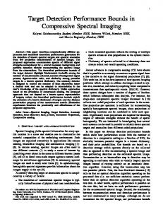
Figure 1. Model overview of the insect-inspired tracker (IIT). The model includes: 1) Early visual processing which simulates the spectral sensitivity, optical blur and low resolution sampling of the insect visual system. 2) Target matched filtering or Elementary Small Target Motion Detector (ESTMD) provides selectivity for small moving targets: separation of OFF and ON channels, fast temporal adaptation, strong surround antagonism and temporal correlation between opposite contrast polarity channels. 3) The facilitation mechanism which is observed in dragonfly CSTMD1 neurons was modelled by building a weighted map (FG(r'), supplementary material, Fig. S1) based on the predicted location of the target in the next sampling time (r'(t+1)). The predicted target location was calculated by shifting the location of the winning feature (r(t)) with an estimation of the target velocity vector (v(t)) provided by the Hassenstein-Reichardt elementary motion detector which was multiplied with sampling time (Ts). The facilitation mechanism multiplies the winning output of ESTMDs (maximum) with a delayed (z-1) version of a weighted map based on the current location of the winning feature but offset in the direction of the target’s movement. The time constant of the facilitation low-pass filter controls the duration of the enhancement around the winning feature.
5
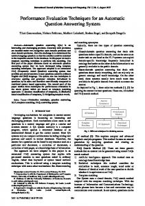
Figure 2. Output of model stages, including optics, large monopolar cells (LMC) and elementary small target motion detector (ESTMD). The red rectangle in the input image shows the bounding box of the target.
2.1.3 Integration and facilitation A hyperbolic tangent function was used to model the neuronlike soft saturation of ESTMD outputs, ensuring a signal range between 0 and 1:
𝑠(𝑥) =
Figure 3. Fast adaptation algorithm (FA). The half-wave rectified channels ‘u’, is fed into the ‘Gradient Check’ block (Eq. 6), which determines whether the luminance of each individual pixel is rising or falling, and outputs a matrix of appropriate ‘τ’ (time constant) values. Both ‘u’ and ‘τ’ are fed into the FA low-pass filter block, which filters each pixel of the image according to the time constant value. The filtered image ‘v’ is subtracted from the original image ‘u’. This computation emulates fast temporal adaptation, reducing responses to textural variations in the image.
Kernel S -1 -1 -1 -1 -1
Kernel M -1 -1 -1 -1 -1
Kernel L -1 -1 -1 -1 -1
-1 -1 -1 -1 -1
-1 0
-1 2
-1 -1 2 -1 -1 -1 -1 -1 -1 -1 -1 -1 -1 -1 -1
-1 0 2 0 -1 -1 0 0 0 -1 -1 -1 -1 -1 -1
0
0 -1
2
2 -1
-1 2 2 2 -1 -1 2 2 2 -1 -1 -1 -1 -1 -1
Figure 4. The kernels that are used in centre-surround antagonism (CSA) to change model size-tuning.
𝑒 𝑥 −𝑒 −𝑥 𝑒 𝑥 +𝑒 −𝑥
.
(9)
A simple competitive selection mechanism is added to the target detection algorithm by choosing the maximum of all ESTMD output values sampling the visual field. The location of this maximum in the ESTMD output is considered as the target location. The slow build-up of facilitation as observed in dragonfly CSTMD1 neurons (Nordström et al., 2011; Dunbier et al., 2011; Dunbier et al., 2012) permits the extraction of the target signal from noisy (cluttered) environments (Bagheri et al., 2015). Previously, we modelled this facilitation mechanism with a Gaussian weighted ‘map’, located relative to the winning feature, shifted to account for the target’s velocity (Bagheri et al., 2015). Here we implement facilitation with a retinotopic array of small-field STMDs, each integrating ESTMD output (~10°x10° region) with weights defined by a grid of 2D Gaussian kernels (half-width at half maximum of 5°) with centres separated by 5° (50% overlap) (Supplementary Materials, Fig. S1). To mimic the slow build-up of the response of CSTMD1 neurons the ESTMD output was multiplied with a low-pass filtered version of this facilitation map (Ts=0.001 ms). 𝑧+1 𝐿𝑃𝐹𝑎𝑐 = , (10) 40 40 (1 + ) 𝑧 + (1 − ) 𝑤 𝑤 by changing w we varied the time constant of this discrete lowpass filter (facilitation time constant), thus controlling the duration of enhancement around the predicted location of the winning feature. We previously showed that the optimal
6 facilitation time constant is dependent on the amount of background clutter and the target’s velocity (Bagheri et al., 2015). In physiological recordings, we observe variability in individual response time-courses (mean ~200 ms), suggesting variability in facilitation time constants and modulatory factors that may dynamically change this parameter are currently under investigation. Here, we approximated this variability by determining the optimum facilitation time constant for each data sequence, testing across the range 40 to 2000 ms (9 values). The directional component of the velocity vector was provided using a traditional bio-inspired direction selective model; the Hassenstein-Reichardt elementary motion detector (HR-EMD) (Hassenstein and Reichardt, 1956). The HR-EMD (Fig. 5a) was applied to the ESTMD outputs, correlating two adjacent inputs, one after a delay (via a low-pass filter, τ=40 ms, Ts=0.001 ms): 𝐿𝑃𝐻𝑅−𝐸𝑀𝐷 =
𝑧+1 . 9𝑧 − 7
(11)
This results in a direction-selective output that is tuned to the velocity of small objects (Wiederman and O'Carroll, 2013b). The output of HR-EMD will be positive when the target moves from S1 to S2 (Fig. 5a), and negative in the reverse direction. The HR-EMD was applied in both horizontal and vertical directions to estimate whether the target is moving right/up (positive) or left/down (negative). The spatial shift of the facilitation kernel was determined by binning the magnitude of the output of the HR-EMD into three equal intervals, to estimate whether the speed of the target is slow, medium or fast (Bagheri et al., 2015). Fig. 5b shows how this facilitation map builds up throughout tracking. 2.2 Input Imagery 2.2.1 High contrast target The ESTMD model is size-tuned, due to spatial centresurround antagonism and temporal cross correlation between local ON and OFF pathways. This forms a ‘matched filter’ for both the spatial and temporal characteristics of small, moving features. Additionally, the model has inherent velocity tuning as observed in correlation-type motion detection mechanisms (i.e. HR-EMD). The position of the peak velocity response is dependent on the ON/OFF delay filter time constant as seen in Fig. 1. We quantified this model tuning by presenting high contrast (black on white) targets of varying size and velocity. 2.2.2 Large targets within natural scenes The IIT model was designed to detect small moving targets, in the order of a few degrees. However, because large objects may be composed of several small parts, we examined what the IIT model would do when presented with a range of object sizes. To test such scenarios, we used the CVPR2013 Online Object Tracking Benchmark (OOTB) (Wu et al., 2013). This is a popular and comprehensive benchmark dataset of 50 sequences with a manually generated ground truth for each frame, specifically designed for evaluating performance. The field of view (FOV) for these sequences was not available, therefore our 1° subsampling was implemented assuming capture by a 35 mm (equivalent) camera with a normal 50 mm lens (average diagonal FOV~55°). Fig. 6a shows a 2-D
histogram of target size and velocity within OOTB. This reveals that only a small proportion of targets within the OOTB dataset is within the tuning range of IIT (see Section 3.1). 2.2.3 Small targets within natural scenes To match our problem definition, i.e. tracking small, moving targets in natural scenes, we recorded 25 additional video sequences (STNS Dataset). These sequences included heavy background clutter and camera motion. The statistical properties of the targets within these video sequences are presented in Fig. 6b. The range of target size and velocity presented in the STNS dataset is one typically required for applications such as airborne surveillance. Datasets varied from 71 to 3872 frames, with an average of 760. These video sequences are available online, including the manually generated ground truth for each frame (https://figshare.com/articles/STNS_Dataset/4496768). The datasets we used here contained a range (and type) of background motion including translation, rotation, and vibration. Although due to the lack of depth perception we could not quantify the motion in the direction perpendicular to the image plane, the camera motion in the image plane in these sequences ranges from a stationary camera (0 °/s) to an average camera velocity of 22±8 °/s. 2.3 Benchmarking Algorithms To establish the efficacy and computational efficiency of our insect-inspired tracker (IIT) model, we compared its performance with three recent models DSST (Danelljan et al., 2014), KCF (Henriques et al., 2015), and MUSTer (Hong et al., 2015) as well as six ‘classic’, highly-cited algorithms. We chose MATLAB implementations of these algorithms (provided by their authors), to maximise the fairness of comparison. The Matlab code for the IIT model is downloadable via https://figshare.com/s/377380f3def1ad7b9d44. 1- Discriminative Scale Space Tracker (DSST) (Danelljan et al., 2014) proposes a separate 1dimensional correlation filter to estimate the target scale. This model uses the original feature space as the object representation. 2- Kernelised correlation filter (KCF) tracker (Henriques et al., 2015) uses multiple channels by summing over the results from all the channels in the Fourier domain. This model boosts its performance by using a Gaussian kernel and histogram-of-oriented-gradients (HOG) features. 3- MUlti-Store Tracker (MUSTer) (Hong et al., 2015) proposes a cooperative tracking framework inspired by a biological memory model called the Atkinson Shiffrin Memory Model (ASMM) (Atkinson and Shiffrin, 1968). ASMM is inspired by short-term and long-term memory in the human brain. Short-term memory which updates aggressively and forgets information quickly, stores local and temporal information. However, long-term memory which updates conservatively and maintains information for a long time, retains general and reliable information.
7
Figure 5. a) The Hassenstein-Reichardt (HR) EMD uses two spatially separated contrast signals (S1, S2) and correlates them after a delay (LP, low-pass filter) resulting in a direction selective output (Hassenstein and Reichardt, 1956). Subtracting the two mirrored symmetric sub-units yields positive response for the preferred motion direction (in this case left to right) and a negative one in the opposite direction (right to left). b) The facilitation map builds up slowly in response to targets that move along long, continuous trajectories. Therefore, as the tracking progresses, the facilitation map builds in strength around the selected target.
4- Compressive Tracking (CT) (Zhang et al., 2012) proposes an appearance model based on features extracted in the compressed domain. This tracker uses a sparse measurement matrix to extract the features for the appearance model. 5- Incremental Visual Tracker (IVT) (Ross et al., 2008) proposes an adaptive appearance model. This tracker calculates and stores the Eigen images of the latest target observation with incremental principal component analysis (IPCA) while slowly deletes the old observations. 6- L1-minimization Tracker (L1T) (Mei et al., 2011) employs sparse representation by L1 to provide an occlusion insensitive method. This tracker uses a particle filter to find target windows. Then it defines sparse representation by using the intensity of sample windows close to the target location. 7- Locally Orderless Tracker (LOT) (Oron et al., 2012) divides the initial bounding box into super pixels. Each super pixel is represented by its centre of mass and average HSV-value. This tracker employs a parameterized Earth Mover Distance (Rubner et al., 2000) between the super pixels of the candidate and the target windows to calculate the likelihood of each particle sample. 8- Super Pixel Tracker (SPT) (Wang et al., 2011) clusters super pixels based on their histograms to form a discriminative appearance model for distinguishing the object from the background. 9- Tracking, Learning and Detection (TLD) (Kalal et al., 2012) combines a discriminative learning method with a
detector and a Median-Flow tracker. The learning process uses a pair of false positives and false negatives experts to estimate the errors of the detector and to avoid these errors in future observations. All models were tested in MATLAB on the same PC with a 4-core Intel i7 3770 CPU (3.4 GHz) and 16 GB RAM. The location of a target bounding box in the initial frame was provided for the benchmark algorithms. Likewise, in the first frame, we biased our IIT model toward the initial location of the target by allowing the facilitation to build up in the target region for 200 ms prior to the start of the experiment. This was implemented by feeding the target location in the first frame as the future location of the target (r’(t+1) in Fig. 1) to the facilitation mechanism.
8
Figure 6. 2D histograms of dataset statistics showing the target size and velocity range in the tested datasets. The OOTB dataset has a broader range of objects at larger sizes, that move at slower speeds. Our problem definition is the tracking of small, moving targets as created in the STNS dataset (~5°, ~20-70°/s).
3
RESULTS
Here, we present our measures of robustness and processing speed for the group of trackers. The protocol is to initialize the tracker in the first frame and then track the object of interest until the last. The resultant trajectory is compared to ground truth using metrics as specified in each experiment.
3.1 Size and Velocity Tuning An important feature of our model is its size and velocity tuning. The addition of facilitation increases target discriminability, but also modifies model size and velocity tuning. We quantified this tuning (Fig. 7) to investigate the relationship between model responses and target properties within the input imagery. We varied facilitation time constants in addition to a non-facilitated model. The model displays maximum responses at a target size of ~3-4°, diminishing above 10º. The model does not respond to targets slower than 20º/s and the optimum velocity increases as target size increases. This is due to the increased spatial separation between leading and trailing edges (in the direction of travel), which requires a faster transit speed to match the correlation delay between OFF and ON channels (confounding target width and velocity, as observed in physiology). This relationship between velocity and size might be beneficial in closed-loop pursuit as the insect approaches its target. Fig. 7 shows facilitation changes the size and velocity tuning of the model. While the non-facilitated model responds to target sizes of up to 14º, facilitation broadens the tuning range to 27º at high target velocities (V>200º/s, facilitation time constant τ=40 ms). The shorter the facilitation time constant is, the faster facilitation builds up to its maximum (Bagheri et al., 2015), therefore, model responses increase as facilitation time constant decreases. However, the choice of optimum facilitation time constant is complicated since it depends on different factors such as target velocity and background image statistics (Bagheri et al., 2015). 3.2 Size Tuning Fig. 8 shows tracking snapshots for each sequence, representative of early, middle and late stages of the tracking. In OOBT sequences, our IIT model selects sub-features of the large object within its tuning size, and retains that selection throughout the tracking. For example, in the Couple sequence the model locks on to the shoes of the pedestrians, in the Mountain Bike sequence it focuses on the bike seat and in the Jogging sequence it follows the head of the jogger. However, in the sequences belonging to the STNS dataset (Key, Train, Pony2, Owl2), where the target is already within the size tuning, it tracks the object itself.
9
Without Facilitation
Facilitation Time Constant =40 ms 1
Target Diagonal (°)
30 25 0.2
20
0.4
0.8 0.6
15 0.2
10
0.8 0.4
5
1
0.6
0.6
0 Facilitation Time Constant=400 ms
Facilitation Time Constant =100 ms
Target Diagonal (°)
30
0.4
25
Avergae Model Response
0.8 1
0.2
20
0.4
15
0.2 0.4
0.6
0.6
10 0.8
5 0 20
0.2
0.8 1
1
50
100
150
200
250
300 20
Target Velocity (°/s)
50
100
150
200
250
300
0
Target Velocity (°/s)
Figure 7. Size and velocity tuning of the model. The average model response was calculated by varying the size and velocity of a black target moving against a white background for both facilitated (with different time constant) and non-facilitated cases. The maximum response in all cases is for a target of ~3-4° moving at velocity of ~ 70-100 (°/s). However, the optimum velocity increases as the target size increases.
The IIT model was designed to mimic size tuning observed in STMD neurons. However, recent physiological experiments have observed additional STMD types with peak responses for larger objects at ~10° (Wiederman et al., 2013a). This raises the intriguing possibility of parallel pathways encoding different, broadly-tuned size ranges, which might be combined later in the visual pathway for a precise estimate of size (Evans et al., In press). This would be analogous to a human’s capability to encode millions of colour wavelengths, with only three broadly tuned photoreceptor classes. To explore how individual, sizetuned pathways would respond to input imagery, we varied the model’s size tuning by changing the strong spatial centresurround antagonism at the ESTMD stage (Fig. 4). Kernel S (small) provides a stronger surround antagonism compared to Kernel M (medium, the default kernel), hence, the model is selective to smaller features. Kernel L (large) tunes the model to larger objects. Fig. 9 shows how the size tuning range of the model changes with different kernels and Fig. 10 provides examples of the sub-features tracked with different kernels. For instance, in the Jogging sequence, the model locks on to the head (~3.6°) with Kernel M. However, the model is able to
select other features, such as, a shoe (Kernel S, ~1°) and the jogger’s pants (Kernel L, ~7°). We measured success rate as the frame percentage where the target is correctly identified by the tracker. Target size and orientation could be useful information in some applications. However, for our purpose, targets are a small square (i.e. equal to its subsampling resolution) and we limit our success metric to correctly locating target position in each frame. For the IIT algorithm, if the location of the winning feature was within the ground truth box of the whole target, it was considered a successful detection of the target. Fig. 11 shows box-and-whiskers plots summarizing how the size tuning of the model influences the success rate. The central mark (white circle) is median success rate, edges are the 25th and 75th percentiles, and whiskers are the non-outlier data range. For the OOTB dataset, which has generally larger targets, the success rate of the model increases with a kernel selected for larger objects (Kernel L). In contrast, for the STNS dataset which uses small targets deliberately designed to match the relative size of typical prey pursued by predatory dragonflies,
10 Kernel S leads to a more robust model performance. Kernel M provides a trade-off between selectivity to large features and small features. Consequently, the success of the IIT model with Kernel M is between those for Kernel S and Kernel L. For the remaining analysis, we use the result of experiments with Kernel M. 3.3 Facilitation Time Constant Our previously published work (Bagheri et al., 2015) show that the optimum facilitation time constant varies systematically with image statistics and target velocity, suggesting that a dynamic modulation of time constant would improve target detection. However, in the current version of the model rather than implementing a dynamic control system for the time constant, we simply used several variants. We also tested the model with a global optimum facilitation time constant (τf=400 ms). Fig. 12 shows the difference between median of these two implementations is not significant (less than 1.5%). However, using a global optimal time constant (IIT) diminishes the 25th and 75th percentile by ~8% compared to the implementation with suboptimal time constant for each data sequence (IIT*). In the following sections, we used the results of experiments with optimum time constant for each data sequence. 3.4 Benchmarking Success Plot In computer vision literature, target detection is typically represented with a bounding box, with a common measure for success being a 50% overlap between the ground truth box and target bounding box (Wu et al., 2013; Smeulders et al., 2014).
Here we scored each frame as a success if the bounding box centre was within the target ground truth box. Although this provides a higher success rate than the common success measure, since our model represents the target with a small square, we used this metric to provide a fairer comparison between our model and the other engineering models. Fig. 12a shows OOTB dataset results which mainly consists of large targets (see Methods 2.2.2). The median of IIT*, CT, IVT, LOT and SPT are similar though all fall far behind the state-of-the-art trackers such as DSST, KCF and MUSTer. This is unsurprising, given our model is designed to track small moving targets in natural scenes, whilst the OOBT dataset is composed of many larger objects that are, in effect, false positives for our model design. Of interest, is that in the OOBT dataset, the IIT model often tracks smaller components of a large object. Whether the combination of parallel size-tuned pathways could be utilized to track OOBT objects is currently being investigated. In comparison to the public dataset, our STNS dataset explores another set of challenges; tracking small moving targets that are frequently camouflaged against the background clutter from a moving platform. In this more challenging set of scenarios, the median performance of all trackers (Fig 12b.) are lower than the OOTB dataset. Although the 75th percentile of our model is not as high as other trackers, it has the highest median and 25th percentile showing its more robust and reliable performance in the most challenging of these scenarios.
11
Figure 8. Snapshots of IIT tracking results in three different frames representing early, middle and late stages for each sequence. The red square marks the location of the winning feature in the output of the IIT model.
12
Figure 9. The size tuning range of the model changes with the choice of kernel for strong spatial centre-surround antagonism at the ESTMD stage. With Kernel S the model is selective for small targets and Kernel L tunes the model to larger objects. Kernel M provides a trade-off between selectivity to large features and small features. The average response of the model was measured for a black target moving against white background at velocity of 100 °/s with a facilitation time constant of 40 ms.
Figure 10. Different kernels for centre-surround antagonism change size tuning of the model and consequently sub-features of the target that the model selects for tracking. The red square marks the location of the winning feature in the output of the IIT model.
3.5 Precision Plot The Precision plot is an evaluation method recently adopted to measure the robustness of tracking (Wu et al., 2013; Danelljan et al., 2014; Henriques et al., 2015; Homg et al., 2015; Babenko et al., 2011). It shows the percentage of the frames where the Euclidean distance between the centre of the tracked target and the ground truth is within a given ‘location error’ threshold (Fig. 13). A higher precision at low thresholds means the tracker is more accurate. Precision at a 20 pixel threshold is widely used as a performance benchmark in the literature (Wu et al., 2015; Henriques et al., 2015; Babenko et al., 2011). Fig. 14a shows the precision plot for all trackers both for OOTB and STNS datasets. In the OOTB dataset our IIT model has a low precision until the threshold of 11 pixels. Nonetheless, its precision catches up to SPT, CT, L1T and IVT, LOT and TLD around the threshold of 16 pixels. However, its precision never nears DSST, KCF or MUSTer. In contrast, in the experiments with the STNS dataset, the precision of our model exceeds the precision of all trackers at a threshold of 30 pixels. The poor precision of our model below the threshold of 16 pixels with the OOTB dataset is due to two factors. Firstly, large objects are composed of small contrasting parts, allowing our model to lock on to these sub-features of the larger object. The result is robust target tracking, but with the location of the tracked feature typically offset from the centre of the object.
Figure 11. Effect of size tuning on model performance. Tuning to larger objects increases the model success rate in the OOTB dataset, however, it diminishes model performance in the STNS dataset. This is because the OOTB dataset is biased to large objects, whereas the STNS dataset has small moving targets.
13
Figure 13. Schematic of the mechanism that is used for calculation of precision. The green arrow (d) shows the ‘location error’ between the centre of the ground truth and winning feature. The white arrow (D) shows half of the diagonal of the ground truth rectangle which is used for normalization. Therefore, the normalized location error is equal to d/D.
Figure 12. Box and whiskers plots for successful target tracking of different algorithms for a) OOTB dataset, b) our own dataset (STNS dataset). The white circles represent the median success rate, and the box shows the 25th and 75th percentile. The IIT and IIT* present the results with a global optimum time constant and optimum time constant for each sequence, respectively. The success of IIT model
is the result of experiments with Kernel M.
The second factor is the subsampling of the input image. In Fig. 14a the grey rectangular area shows the location error thresholds below the average subsampling ratio that is applied to the images. This shows our model precision improves as it gets closer to the boundary of the grey region. Although subsampling reduces the redundant information in the scene and increases the processing speed, it also reduces model spatial resolution – a situation that mimics the low spatial acuity of dragonfly compound eyes. However, whether a high spatial acuity is necessary or not is generally application dependent. For example, in applications such as face tracking and gesture recognition in a crowded scene where the target representation is very important, an accurate detection of the target is desirable. Nonetheless, in aerial video surveillance where the target motion and ego-motion of the camera are the more important components, high spatial acuity is not necessary as long as the tracker detects the correct location of the target. Although the precision at a 20 pixel threshold has been used for benchmarking in the literature, this somewhat arbitrary benchmark threshold does not tell the whole story. A 20 pixel offset is a relatively large error for tracking a small object (e.g. on the scale of pixels themselves), yet may not be at all significant for identifying a large object. Therefore, to account for the huge range of target sizes in these image sequences we also normalized the location error of the target in each frame by half of the diagonal of the ground truth rectangle within that frame (Fig. 13). Fig. 14b shows the results of this normalization. Similar to the precision plot in the OOTB dataset our model provides an average level of precision compared to other algorithms. However, in the STNS dataset, over the entire upper 1/2 of this normalized error threshold (NT) our model is substantially more precise, revealing the successful identification of the correct small target location.
14
Figure 14. a) Precision plot for both OOTB and STNS datasets. The grey area shows the location error thresholds below the average subsampling ratio that is applied to the images in the IIT model. b) The precision of the trackers is normalized by half of the diagonal of the ground truth rectangle.
3.6 Overall Performance Table 2 provides a descriptive summary of algorithm performance with the OOTB and STNS datasets. The average success represents the performance across all videos in each dataset (nOOTB=50, nIIT=25). In addition to the average success rate of the sequences, we also calculated the weighted success which shows the percentage of the successful frames out of all the tested frames in each dataset (FOOTB=29518, F STNS=27514). This normalization accounted for the difficulty of ‘long term’ tracking, where it is easier for the trackers to lock on to the target in a short sequence than a long one. Since our STNS dataset mainly includes small moving targets within heavily cluttered environments, the target is frequently well camouflaged against the background clutter.
Therefore, it is more difficult for trackers to lock on to the target. This might explain why the weighted success of all the engineering algorithms for the STNS dataset are lower than their average success (Table 2). However, in both datasets, the weighted success of our model is higher than its average success. Our facilitation mechanism (based on the recently observed facilitatory behaviour of target-detecting neurons (Nordström et al., 2011; Dunbier et al., 2011; Dunbier et al., 2012)) builds up slowly in response to targets that move in long continuous trajectories, and thus improves target detection as tracking progresses (Bagheri et al., 2015). Overall, in the experiments with the OOTB dataset, while it does well, the performance of our IIT model does not exceed those of classical trackers such as CT, IVT, L1T, LOT, SPT and
15 TLD. However, in the STNS dataset, our model outperforms all other trackers in terms of average success, weighted success, and normalized precision. 3.7 Processing Speed In addition to tracking performance, processing efficiency is a critical concern in target tracking applications. Indeed, many trackers are considered impractical in real-time scenarios due to the long processing duration required using typical hardware (Yang et al., 2011; Zhang et al., 2012; Yilmaz et al., 2006). Fig. 15 shows the calculated processing speed for all algorithms using the author-provided MATLAB code. The processing speed is consistent with values reported in the original papers of these algorithms. The most computationally expensive process that applies to images in the IIT model is the Gaussian optical blur in the early visual processing stage. However, previous studies have shown that a Gaussian blur can directly be obtained via optics (Brückner et al., 2006; Colonnier et al., 2015). Likewise, our software implementation of the optical blur built in to biological eyes could be readily implemented by using de-focusing optics in robotic applications. Therefore, we tested the processing speed of our IIT algorithm both with and without optical blur. Even with the processing time required for optical blur the speed of the IIT has the second best median among all trackers. However, when we eliminate the processing time for optical blur, the IIT model exceeds all other trackers, with an average performance approximately 2 times faster than the fastest engineering algorithm (KCF) (note the logarithmic scale in Fig. 15). 3.8 Complexity of Algorithms Although we presented the processing speed of algorithms for the tested sequences, the size of the input image can affect the processing speed of the models. Therefore, to identify how the processing time of these algorithms changes as the problem size increases, we determined the Big O notation (Bach and Shallit, 1996) for our IIT model as well as some of the fastest processing engineering models. The Big O notation characterizes functions according to their growth rates. For the IIT model there are two factors that can change the processing speed and therefore the complexity of the model. The first one is the size of the input image, which mainly affects the processing speed due to the Gaussian optical blur in the early visual processing stage. However, as we mentioned in Section 3.7, this optical blur can be achieved via hardware rather than software. The other factor is the Field of View (FOV) which changes the processing speed after optical blur. Table 3 summarizes the results of the complexity analysis. Although the complexity of the IIT model is quadratic in response to the changes of input image size, the processing time changes linearly in response to variation of FOV. We should mention that we made no attempt to optimize our MATLAB code (e.g. it does not use parallel computation). 4.
CONCLUSION
We have demonstrated the robustness and efficiency of a target-tracking algorithm inspired directly by insect neurophysiology. As with the dragonfly, our model is particularly suited to tracking small moving targets, rather than some of the larger objects within the public OOTB dataset.
Model performance for this task is improved with different tuning kernel weights (Fig. 4 and Fig. 11) and in future research we will test the effect of integrating parallel, size-tuned subsystems. This elaboration may improve precision and yet still retain the real-time performance inherent in our model approach. Although there is no definitive evidence for such parallel processing in insect vision, this processing is wellsupported in human psychophysics experiments (Graham and Nachmias, 1971). How an insect integrates the information of these small moving features across the visual field to detect larger objects is a question physiologists are currently investigating. Nevertheless, in terms of processing speed, our model is one of the best among all the tested trackers, mimicking the remarkable efficiency of the insect visual system upon which it is based. As such, it may be well suited to applications where efficiency is paramount. This is the first time that an insect-inspired target tracking algorithm has been directly tested against state-of–the-art engineered systems. One prior study (Shoemaker et al., 2011) compared an insect-inspired optic flow processing algorithm with computational optic flow estimates based on LucasKanade equations, both in closed loop simulation. As with our own model, their insect inspired system (Shoemaker et al., 2011) was computationally highly efficient and with sufficient elaboration was shown to be robust for certain closed-loop control robotic applications. However, in absolute performance terms, it never surpassed the engineered solution. Perhaps the conclusion of our current work is that despite the relatively simple feed-forward mechanism we implemented, the performance of our system exceeds all other trackers in the scenarios where the target is within its tuning range (i.e., when tracking small objects on the scale of the camera resolution). Nonetheless, our results show that this performance does not come at the cost of additional processing time and the model processes the frames at high speed, especially when the optical blur process is obtained via defocusing optics rather than software implementation. Our previous modelling efforts suggest that the temporal optima of facilitation mechanism varies with respect to the amount of background clutter and target velocity (Bagheri et al., 2015). One of the limitations of the current work is that it uses a static facilitation time constant. Therefore, we simply used several variants of facilitation time constant to find the optimum for each sequence. However, for future robotic applications, an interesting extension of the model would be a system which dynamically modulates the facilitation time constant during run-time. For instant, a fast processing system such as Fuzzy control can be exploited to estimate the facilitation time constant using target velocity (as estimated by the velocity estimator) and background clutter (e.g. using a simple metric for visual clutter such as the one developed by Silk (1995)). Since fuzzy control system uses a set of logical rules to estimate the output, it is well suited for low-cost implementations and would cause very little overhead in terms of execution time.
16
STNS Dataset
OOTB Dataset
Table 2. Summary of experimental results on both OOTB dataset and STNS dataset. Performance Measure Average Success (%) Weighted Success (%) Precision (20 px) Normalized Precision (NT=1) Average Success (%) Weighted Success (%) Precision (20 px) Normalized Precision (NT=1)
IIT 52.0
DSST 78.3
KCF 78.0
MUSTer 89.4
Algorithm CT IVT 51.0 52.9
L1T 45.1
LOT 57.1
SPT 44.6
TLD 55.0
60.0
85.0
87.5
94.3
62.8
60.6
51.5
69.3
47.8
70.0
0.56 0.78
0.81 0.94
0.83 0.94
0.92 0.99
0.42 0.78
0.56 0.70
0.44 0.74
0.61 0.80
0.34 0.73
0.62 0.80
47.6
41.5
33.2
36.4
37.3
42.7
15.0
40.5
41.9
35.0
52.1
34.5
29.9
36.8
32.7
35.8
14.2
40.0
35.9
32.2
0.41 0.57
0.44 0.51
0.27 0.35
0.32 0.44
0.29 0.37
0.25 0.34
0.12 0.22
0.37 0.44
0.32 0.39
0.29 0.41
strategies in a robotic platform to test the performance of them together under real-world conditions. ACKNOWLEDGMENT This research was supported under Australian Research Council's Discovery Projects (DP130104572) and Discovery Early Career Researcher Award (DE15010054) funding scheme, and the Swedish Research Council (VR 2014-4904). We thank the manager of the Botanic Gardens in Adelaide for allowing insect collection and video capture. REFERENCES [1]
Figure 15. Processing speed of trackers. IIT1 and IIT2 represent the model with and without optical blur processing time, respectively. Table 3. The computational complexity of algorithms. IIT1 and IIT2 represent the complexity of IIT model in terms of change in the size of input image and size of FOV, respectively.
Algorithm
IIT1
IIT2
KCF
CT
DSST
TLD
Complexity
O(n2)
O(n)
O(n3)
O(n)
O(n)
O(n2)
Here, we tested our algorithm in open-loop, however, animals interact with the target by changing eye or body movements, which then modulate the visual inputs underlying the detection and selection task (via closed-loop feedback). This active vision system may be a key to further exploiting visual information by the simple insect brain for complex tasks such as target tracking. Future research will attempt to implement this model along with insect active vision gaze-control
Abdel-Hakim A. E., & Farag A. A. (2006). CSIFT: A SIFT descriptor with color invariant characteristics. In 2006 IEEE Computer Society Conference on Computer Vision and Pattern Recognition, 2, 1978-1983. [2] Atkinson R. C., & Shiffrin R. M. (1968). Human memory: A proposed system and its control processes. Psychology of Learning and Motivation, 2, 89-195. [3] Babenko B., Yang M. H., & Belongie S. (2011). Robust object tracking with online multiple instance learning. IEEE Transactions on Pattern Analysis and Machine Intelligence, 33(8), 1619-1632. [4] Bach E., & Shallit J. O. (1996). Algorithmic Number Theory: Efficient Algorithms (Vol. 1). MIT press. [5] Bagheri Z. M., Wiederman S. D., Cazzolato B. S., Grainger S., & O'Carroll D. C. (2015). Properties of neuronal facilitation that improve target tracking in natural pursuit simulations. Journal of The Royal Society Interface, 12(108), 20150083. [6] Bagheri Z. M., Wiederman S. D., Cazzolato B. S., Grainger S., & O'Carroll D. C. (2014a). A biologically inspired facilitation mechanism enhances the detection and pursuit of targets of varying contrast. In International Conference on Digital Image Computing: Techniques and Applications (DlCTA), 1-5. [7] Bagheri Z., Wiederman S. D., Cazzolato B. S., Grainger S., & O'Carroll D. C. (2014b). Performance assessment of an insect-inspired target tracking model in background clutter. In International Conference on Control Automation Robotics & Vision (ICARCV), 822-826. [8] Bar-Shalon Y. and Fortmann T. (1988). Tracking and data Association. Academic Press Professional, Inc. San Diego, CA, USA. [9] Bay H., Tuytelaars T., & Van Gool L. (2006). Surf: Speeded up robust features. In European Conference on Computer Vision, 404-417. [10] Black M. J., & Jepson A. D. (1998). Eigentracking: Robust matching and tracking of articulated objects using a view-based representation. International Journal of Computer Vision, 26(1), 63-84. [11] Blum A., & Mitchell T. (1998). Combining labeled and unlabeled data with co-training. In Proceedings of the 11th Annual Conference on Computational Learning Theory, 92-100.
17 [12] Brückner A., Duparré J., Bräuer A., & Tünnermann A. (2006). Artificial compound eye applying hyperacuity. Optics express, 14(25), 1207612084. [13] Burghouts G. J., & Geusebroek J. M. (2009). Performance evaluation of local colour invariants. Computer Vision and Image Understanding, 113(1), 48-62. [14] Chapelle O., Schölkopf B. & Zien A., (2006). Semi-supervised learning. MIT Press, Cambridge, Massachusetts, USA, 2006. [15] Chen J., Shan S., He C., Zhao G., Pietikainen M., Chen X., & Gao W. (2010). WLD: A robust local image descriptor. IEEE Transactions on Pattern Analysis and Machine Intelligence, 32(9), 1705-1720. [16] Comaniciu D., Ramesh V., & Meer P. (2003). Kernel-based object tracking. IEEE Transactions on Pattern Analysis and Machine Intelligence, 25(5), 564-577. [17] Colonnier F., Manecy A., Juston R., Mallot H., Leitel R., Floreano D., & Viollet S. (2015). A small-scale hyperacute compound eye featuring active eye tremor: application to visual stabilization, target tracking, and short-range odometry. Bioinspiration & Biomimetics, 10(2), 026002. [18] Corbet P. S. (1999). Dragonflies: Behaviour and ecology of Odonata. Cornell University Press, Ithaca, New York. [19] Danelljan M., Häger G., Khan F., & Felsberg M. (2014). Accurate scale estimation for robust visual tracking. In British Machine Vision Conference, 1-5. [20] Dunbier J. R., Wiederman S. D., Shoemaker P. A., & O'Carroll D. C. (2011). Modelling the temporal response properties of an insect small target motion detector. In IEEE International Conference on Intelligent Sensors, Sensor Networks and Information Processing (ISSNIP), 125130. [21] Dunbier J. R., Wiederman S. D., Shoemaker P. A., & O'Carroll D. C. (2012). Facilitation of dragonfly target-detecting neurons by slow moving features on continuous paths. Frontiers in Neural Circuits, 6, 79. [22] Evans B. J. E., O’Carroll D. C., & Wiederman S. D., (In Press). Salience invariance with divisive normalization in higher order insect neurons. 6th European Workshop on Visual Information Processing, EUVIP. [23] Felzenszwalb P., McAllester D., & Ramanan D. (2008). A discriminatively trained, multiscale, deformable part model. In IEEE Conference on Computer Vision and Pattern Recognition, 1-8. [24] Gall J., & Lempitsky V. (2013). Class-specific hough forests for object detection. In Decision Forests for Computer Vision and Medical Image Analysis, 143-157. [25] Grabner H., Leistner C., & Bischof H. (2008). Semi-supervised on-line boosting for robust tracking. In European Conference on Computer Vision, 234-247. [26] Graham N., & Nachmias J. (1971). Detection of grating patterns containing two spatial frequencies: A comparison of single-channel and multiple-channels models. Vision Research, 11(3), 251-259. [27] Halupka K. J., Wiederman S. D., Cazzolato B. S., & O'Carroll D. C. (2013). Bio-inspired feature extraction and enhancement of targets moving against visual clutter during closed loop pursuit. In IEEE International Conference on Image Processing (ICIP), 4098-4102. [28] Halupka K. J., Wiederman S. D., Cazzolato B. S., & O'Carroll, D. C. (2011, December). Discrete implementation of biologically inspired image processing for target detection. In IEEE International Conference on Intelligent Sensors, Sensor Networks and Information Processing (ISSNIP), 143-148. [29] Hare S., Saffari A., & Torr P. H. (2011). Struck: Structured output tracking with kernels. In IEEE International Conference on Computer Vision (ICCV), 263-270. [30] Hassenstein, B. & Reichardt W. (1956). Systemtheoretische analyse der zeit-, reihenfolgen-und vorzeichenauswertung bei der bewegungsperzeption des rüsselkäfers chlorophanus. Zeitschrift für Naturforschung B, 11(9-10), 513-524. [31] Henriques J. F., Caseiro R., Martins P., & Batista J. (2015). High-speed tracking with kernelized correlation filters. IEEE Transactions on Pattern Analysis and Machine Intelligence, 37(3), 583-596. [32] Hong Z., Chen Z., Wang C., Mei X., Prokhorov D., & Tao D. (2015). Multi-store tracker (muster): A cognitive psychology inspired approach to object tracking. IEEE Conference on Computer Vision and Pattern Recognition, 749-758. [33] Jansonius N. M., & Van Hateren J. H. (1991). Fast temporal adaptation of on-off units in the first optic chiasm of the blowfly. Journal of Comparative Physiology A, 168(6), 631-637. [34] Javed O., Ali S., & Shah M. (2005). Online detection and classification of moving objects using progressively improving detectors. In IEEE
[35]
[36]
[37]
[38]
[39] [40]
[41]
[42]
[43]
[44] [45] [46]
[47]
[48]
[49]
[50]
[51]
[52]
[53]
[54]
[55]
[56]
[57]
[58]
Computer Society Conference on Computer Vision and Pattern Recognition, 696-701. Kalal Z., Mikolajczyk K., & Matas J. (2012). Tracking-learningdetection. IEEE Transactions on Pattern Analysis and Machine Intelligence, 34(7), 1409-1422. Kitagawa G. (1987). Non-Gaussian state-space modeling of nonstationary time series. Journal of the American statistical association, 82(400), 10321041. Leistner C., Saffari A., Roth P. M., & Bischof H. (2009). On robustness of on-line boosting-a competitive study. In IEEE 12th Computer Vision Workshops, 1362-1369. Levin A., Viola P., & Freund Y. (2003). Unsupervised improvement of visual detectors using co-training. In Proceedings of 9th IEEE International Conference on Computer Vision, 626-633. Li P., Zhang T., & Ma B. (2004). Unscented Kalman filter for visual curve tracking. Image and Vision Computing, 22(2), 157-164. Masnadi-Shirazi H., Mahadevan V., & Vasconcelos N. (2010). On the design of robust classifiers for computer vision. In IEEE Conference on Computer Vision and Pattern Recognition, 779-786. Mei X., Ling H., Wu Y., Blasch E., & Bai L. (2011). Minimum error bounded efficient ℓ 1 tracker with occlusion detection. IEEE International Conference on Computer vision and pattern recognition (CVPR),12571264. Nordström K., & O’Carroll D. C. (2009). Feature detection and the hypercomplex property in insects. Trends in Neurosciences, 32(7), 383391. Nordström K., Bolzon D. M., & O'Carroll D. C. (2011). Spatial facilitation by a high-performance dragonfly target-detecting neuron. Biology Letters, 7(4), 588-592. Nordström K., Barnett P. D., & O'Carroll D. C. (2006). Insect detection of small targets moving in visual clutter. PLoS Biology, 4(3), e54. O'Carroll, D. (1993). Feature-detecting neurons in dragonflies. Nature, 362, 541-543. O'Carroll D. C., & Wiederman S. D. (2014). Contrast sensitivity and the detection of moving patterns and features. Philosophical Transactions of Royal Society B, 369(1636), 20130043. O'Carroll D. C., Barnett P. D., & Nordström K. (2011). Local and global responses of insect motion detectors to the spatial structure of natural scenes. Journal of Vision, 11(14), 20-20. Ojala T., Pietikainen M., & Maenpaa T. (2002). Multiresolution grayscale and rotation invariant texture classification with local binary patterns. IEEE Transactions on Pattern Analysis and Machine Intelligence, 24(7), 971-987. Olberg R. M., Worthington A. H., & Venator K. R. (2000). Prey pursuit and interception in dragonflies. Journal of Comparative Physiology A, 186(2), 155-162. Oron S., Bar-Hillel A., Levi D., & Avidan S. (2012). Locally orderless tracking. IEEE International Conference on Computer vision and pattern recognition (CVPR), 1940-1947. Osorio D. (1991). Mechanisms of early visual processing in the medulla of the locust optic lobe: How self-inhibition, spatial-pooling, and signal rectification contribute to the properties of transient cells. Visual Neuroscience, 7(4), 345-355. Porikli F., Tuzel O., & Meer P., (2006). Covariance tracking using model update based on lie algebra. In IEEE Computer Society Conference on Computer Vision and Pattern Recognition, 728-735. Ross D. A., Lim J., Lin R. S., & Yang M. H. (2008). Incremental learning for robust visual tracking. International Journal of Computer Vision, 77(13), 125-141. Rubner Y., Tomasi C., & Guibas L. J. (2000). The earth mover's distance as a metric for image retrieval. International Journal of Computer Vision, 40(2), 99-121. Saffari A., Godec M., Pock T., Leistner C., & Bischof H. (2010). Online multi-class LPBoost. In IEEE Conference on Computer Vision and Pattern Recognition (CVPR), 3570-3577. Scovanner P., Ali, S., & Shah, M. (2007). A 3-dimensional SIFT descriptor and its application to action recognition. In Proceedings of the 15th ACM International Conference on Multimedia, 357-360. Shoemaker P. A., Hyslop A. M., & Humbert J. S. (2011). Optic flow estimation on trajectories generated by bio-inspired closed-loop flight. Biological Cybernetics, 104(4-5), 339-350. Silk J. D. (1995) Statistical variance analysis of clutter scenes and applications to a target acquisition test. Institute for Defense Analysis, Alexandria, Virginia, 2950.
18 [59] Smeulders A. W., Chu D. M., Cucchiara R., Calderara S., Dehghan A., & Shah, M. (2014). Visual tracking: An experimental survey. IEEE Transactions on Pattern Analysis and Machine Intelligence, 36(7), 14421468. [60] Srinivasan M. V., & Guy R. G. (1990). Spectral properties of movement perception in the dronefly Eristalis. Journal of Comparative Physiology A, 166(3), 287-295. [61] Stavenga D. (2003). Angular and spectral sensitivity of fly photoreceptors. I. Integrated facet lens and rhabdomere optics. Journal of Comparative Physiology A, 189(1), 1-17. [62] Straw A. D., Warrant E. J., & O'Carroll D. C. (2006). A bright zone in male hoverfly (Eristalis tenax) eyes and associated faster motion detection and increased contrast sensitivity. Journal of Experimental Biology, 209(21), 4339-4354. [63] Wang S., Lu H., Yang F., & Yang M. H. (2011). Superpixel tracking. In IEEE International Conference on Computer Vision (ICCV), 1323-1330. [64] Wiederman S. D., & O’Carroll D. C. (2013a). Selective attention in an insect visual neuron. Current Biology, 23(2), 156-161. [65] Wiederman S. D., & O'Carroll D. C. (2013b). Biomimetic target detection: Modeling 2nd order correlation of OFF and ON channels. In IEEE Symposium on Computational Intelligence for Multimedia, Signal and Vision Processing (CIMSIVP), pp. 16-21. [66] Wiederman S. D., & O'Carroll D. C. (2011). Discrimination of features in natural scenes by a dragonfly neuron. The Journal of Neuroscience, 31(19), 7141-7144. [67] Wiederman S. D., Shoemaker P. A., & O'Carroll D. C. (2013). Correlation between OFF and ON channels underlies dark target selectivity in an insect visual system. The Journal of Neuroscience, 33(32), 13225-13232. [68] Wiederman S. D., Shoemaker P. A., & O'Carroll D. C. (2008). A model for the detection of moving targets in visual clutter inspired by insect physiology. PloS One, 3(7), e2784. [69] Wu, Y., Lim, J., & Yang, M. H. (2013). Online object tracking: A benchmark. In Proceedings of the IEEE Conference on Computer Vision and Pattern Recognition, 2411-2418. [70] Yang H., Shao L., Zheng F., Wang L., & Song Z. (2011). Recent advances and trends in visual tracking: A review. Neurocomputing, 74(18), 38233831.
[71] Yilmaz A., Javed O., & Shah M. (2006). Object tracking: A survey. ACM Computing Surveys (CSUR), 38(4), 1-45. [72] Zeisl, B., Leistner C., Saffari A., & Bischof H. (2010). On-line semisupervised multiple-instance boosting. In IEEE Conference on Computer Vision and Pattern Recognition (CVPR), 1879-1879. [73] Zhang K., Zhang L., & Yang M. H. (2012). Real-time compressive tracking. In European Conference on Computer Vision, 864-877. [74] Zhao G., & Pietikainen M. (2007). Dynamic texture recognition using local binary patterns with an application to facial expressions. IEEE Transactions on Pattern Analysis and Machine Intelligence, 29(6), 915928. [75] Zhu X., & Goldberg A. B. (2009). Introduction to semi-supervised learning. Synthesis Lectures on Artificial Intelligence and Machine Learning, 3(1), 1-130.