Algorithms for remote estimation of chlorophyll-a in coastal and inland waters using red and near infrared bands Alexander A. Gilerson,1,* Anatoly A. Gitelson,2 Jing Zhou,1 Daniela Gurlin,2 Wesley Moses,2 Ioannis Ioannou,1 and Samir A. Ahmed1 1
Optical Remote Sensing Laboratory, Department of Electrical Engineering, The City College of the City University of New York, 140 St & Convent Ave, New York, New York 10031 USA 2 Center for Advanced Land Management Information Technologies (CALMIT), School of Natural Resources, University of Nebraska-Lincoln, USA *
[email protected]
Abstract: Remote sensing algorithms that use red and NIR bands for the estimation of chlorophyll-a concentration [Chl] can be more effective in inland and coastal waters than algorithms that use blue and green bands. We tested such two-band and three-band red-NIR algorithms using comprehensive synthetic data sets of reflectance spectra and inherent optical properties related to various water parameters and a very consistent in situ data set from several lakes in Nebraska, USA. The two-band algorithms tested with MERIS bands were Rrs(708)/Rrs(665) and Rrs(753)/Rrs(665). The three-band algorithm with MERIS bands was in the form R3 = [Rrs−1(665) − Rrs−1(708)] × Rrs(753). It is shown that the relationships of both Rrs(708)/Rrs(665) and R3 with [Chl] do not depend much on the absorption by CDOM and non-algal particles, or the backscattering properties of water constituents, and can be defined in terms of water absorption coefficients at the respective bands as well as the phytoplankton specific absorption coefficient at 665 nm. The relationship of the latter with [Chl] was established for [Chl] > 1 mg/m3 and then further used to develop algorithms which showed a very good match with field data and should not require regional tuning. ©2010 Optical Society of America OCIS codes: (010.4450) Ocean optics; (280.0280) Remote sensing.
References and links 1.
2. 3. 4. 5.
6.
7.
G. Moore, J. Aiken, and J. Lavender, “The atmospheric correction of water colour and the quantitative retrieval of suspended particulate matter in Case II waters: application to MERIS,” Int. J. Remote Sens. 20(9), 1713–1733 (1999). J. Aiken, and G. Moore, “ATBD case 2 bright pixel atmospheric correction,” Center for Coastal & Marine Sciences, Plymouth Marine Laboratory, U.K., Rep, PO-TN-MEL-GS 4, 0005 (2000). M. Wang, and W. Shi, “Estimation of ocean contribution at the MODIS near-infrared wavelengths along the east coast of the U.S.: Two case studies,” Geophys. Res. Lett. 32(13), L13606 (2005), doi:10.1029/2005GL022917. M. Wang, and W. Shi, “The NIR-SWIR combined atmospheric correction approach for MODIS ocean color data processing,” Opt. Express 15(24), 15722–15733 (2007). R. Doerffer, and H. Schiller, “MERIS regional coastal and lake case 2 water project atmospheric correction ATBD,” Institute for Coastal Research, GKSS Research Center, Geesthacht, Germany, Rep, GKSS-KOFMERIS-ATB D01, 1 (2008). P. J. Werdell, S. W. Bailey, B. A. Franz, L. W. Harding, Jr., G. C. Feldman, and C. R. McClain, “Regional and seasonal variability of chlorophyll-a in Chesapeake Bay as observed by SeaWiFS and MODIS-Aqua,” Remote Sens. Environ. 113(6), 1319–1330 (2009). A. A. Gitelson, G. Keydan, and V. Shishkin, “Inland waters quality assessment from satellite data in visible range of the spectrum,” Sov. Remote Sens. 6, 28–36 (1985).
#134029 - $15.00 USD
(C) 2010 OSA
Received 25 Aug 2010; revised 25 Oct 2010; accepted 26 Oct 2010; published 3 Nov 2010
8 November 2010 / Vol. 18, No. 23 / OPTICS EXPRESS 24109
8. 9. 10.
11. 12. 13.
14.
15. 16.
17. 18.
19. 20.
21. 22.
23. 24.
25. 26.
27. 28.
29.
30. 31. 32.
33.
R. P. Stumpf, and M. A. Tyler, “Satellite detection of bloom and pigment distributions in estuaries,” Remote Sens. Environ. 24(3), 385–404 (1988). A. A. Gitelson, “The peak near 700 nm on radiance spectra of algae and water: relationships of its magnitude and position with chlorophyll concentration,” Int. J. Remote Sens. 13(17), 3367–3373 (1992). A. A. Gitelson, G. Dall’Olmo, W. Moses, D. C. Rundquist, T. Barrow, T. R. Fisher, D. Gurlin, and J. Holz, “A simple semi-analytical model for remote estimation of chlorophyll-a in turbid waters: Validation,” Remote Sens. Environ. 112(9), 3582–3593 (2008). H. R. Gordon, “Diffuse reflectance of the ocean: the theory of its augmentation by chlorophyll a fluorescence at 685 nm,” Appl. Opt. 18(8), 1161–1166 (1979). A. Vasilkov, and O. Kopelevich, “Reasons for the appearance of the maximum near 700 nm in the radiance spectrum emitted by the ocean layer,” Oceanology (Mosc.) 22, 697–701 (1982). J. F. Schalles, “Optical Remote Sensing Techniques to Estimate Phytoplankton Chlorophyll a Concentrations in Coastal Waters with Varying Suspended Matter and CDOM Concentrations,” in Remote Sensing of Aquatic Coastal Ecosystem Processes: Science and Management Applications, L.L. Richardson and E.F. LeDrew, eds. (Springer, 2006), Chap. 3. G. Dall'Olmo, A. A. Gitelson, and D. C. Rundquist, “Towards a unified approach for remote estimation of chlorophyll-a in both terrestrial vegetation and turbid productive waters,” Geophys. Res. Lett. 30(18), 1938 (2003), doi:10.1029/2003GL018065. L. Han, and D. Rundquist, “Comparison of NIR/Red ratio and first derivative of reflectance in estimating algalchlorophyll concentration: a case study in a turbid reservoir,” Remote Sens. Environ. 62(3), 253–261 (1997). C. Le, Y. Li, Y. Zha, D. Sun, C. Huang, and H. Lu, “A four-band semi-analytical model for estimating chlorophyll a in highly turbid lakes: The case of Taihu Lake, China,” Remote Sens. Environ. 113(6), 1175–1182 (2009). H. J. Gons, M. Rijkeboer, and K. G. Ruddick, “A chlorophyll-retrieval algorithm for satellite imagery (Medium Resolution Imaging Spectrometer) of inland and coastal waters,” J. Plankton Res. 24(9), 947–951 (2002). K. G. Ruddick, H. J. Gons, M. Rijkeboer, and G. Tilstone, “Optical remote sensing of chlorophyll a in case 2 waters by use of an adaptive two-band algorithm with optimal error properties,” Appl. Opt. 40(21), 3575–3585 (2001). J. Gower, S. King, G. Borstad, and L. Brown, “Detection of intense plankton blooms using the 709 nm band of the MERIS imaging spectrometer,” Int. J. Remote Sens. 26(9), 2005–2012 (2005). G. Dall’Olmo, and A. A. Gitelson, “Effect of bio-optical parameter variability on the remote estimation of chlorophyll-a concentration in turbid productive waters: experimental results,” Appl. Opt. 44(3), 412–422 (2005). A. A. Gitelson, J. Schalles, and C. M. Hladik, “Remote chlorophyll-a retrieval in turbid productive estuarine: Chesapeake Bay case study,” Remote Sens. Environ. 109(4), 464–472 (2007). G. Dall’Olmo, and A. A. Gitelson, “Effect of bio-optical parameter variability and uncertainties in reflectance measurements on the remote estimation of chlorophyll-a concentration in turbid productive waters: modeling results,” Appl. Opt. 45(15), 3577–3592 (2006). C. D. Mobley, Light and Water. Radiative Transfer in Natural Waters (Academic Press, New York, 1994). A. Gilerson, J. Zhou, S. Hlaing, I. Ioannou, J. Schalles, B. Gross, F. Moshary, and S. Ahmed, “Fluorescence component in the reflectance spectra from coastal waters. Dependence on water composition,” Opt. Express 15(24), 15702–15721 (2007). Z. P. Lee, http://www.ioccg.org/groups/OCAG_data.html. A. M. Ciotti, M. R. Lewis, and J. J. Cullen, “Assessment of the relationships between dominant cell size in natural phytoplankton communities and the spectral shape of the absorption coefficient,” Limnol. Oceanogr. 47(2), 404–417 (2002). A. Bricaud, M. Babin, A. Morel, and H. Claustre, “Variability in the chlorophyll-specific absorption coefficients of natural phytoplankton: Analysis and parameterization,” J. Geophys. Res. 100(C7), 13321–13332 (1995). A. A. Gitelson, D. Gurlin, W. J. Moses, and T. Barrow, “A bio-optical algorithm for the remote estimation of the chlorophyll-a concentration in case 2 waters,” Environ. Res. Lett. 4(4), 045003 (2009), doi:10.1088/17489326/4/4/045003. W. J. Moses, A. A. Gitelson, S. Berdnikov, and V. Povazhnyy, “Satellite Estimation of Chlorophyll-a Concentration Using the Red and NIR Bands of MERIS—The Azov Sea Case Study,” IEEE Geosci. Remote Sens. Lett. 6(4), 845–849 (2009). H. R. Gordon, O. B. Brown, R. H. Evans, J. W. Brown, R. C. Smith, K. S. Baker, and D. K. Clark, “A semianalytic radiance model of ocean color,” J. Geophys. Res. 93(D9), 10909–10924 (1988). R. C. Smith, and K. S. Baker, “Optical properties of the clearest natural waters (200-800 nm),” Appl. Opt. 20(2), 177–184 (1981). J. Zhou, A. Gilerson, I. Ioannou, S. Hlaing, J. Schalles, B. Gross, F. Moshary, and S. Ahmed, “Retrieving quantum yield of sun-induced chlorophyll fluorescence near surface from hyperspectral in-situ measurement in productive water,” Opt. Express 16(22), 17468–17483 (2008). P. Gege, and A. Albert, “A tool for inverse modeling of spectral measurements in deep and shallow waters,” in Remote Sensing of Aquatic Coastal Ecosystem Processes: Science and Management Applications, L.L. Richardson and E.F. LeDrew, eds. Chap. 4, Springer, 2006.
#134029 - $15.00 USD
(C) 2010 OSA
Received 25 Aug 2010; revised 25 Oct 2010; accepted 26 Oct 2010; published 3 Nov 2010
8 November 2010 / Vol. 18, No. 23 / OPTICS EXPRESS 24110
34. J. E. O'Reilly, and 24 Coauthors, “SeaWiFS Postlaunch Calibration and Validation Analyses, Part 3,” in NASA Tech. Memo. 2000–206892, Vol. 11, S. B. Hooker and E. R. Firestone, eds., (NASA Goddard Space Flight Center, Greenbelt, MD, 2000) 49 pp.
1. Introduction Recent advances in the development of atmospheric correction models [1–5] have made the retrieval of reflectance of coastal and inland waters from electromagnetic signals from the top of the atmosphere more accurate and have inspired further development of retrieval algorithms for turbid productive waters and their analysis [6]. This includes algorithms that employ wavebands in the red and near infrared (NIR) range (650-800 nm), which are less sensitive than traditional blue-green (440-550 nm) ratio algorithms to the absorption by colored dissolved organic matter (CDOM) and scattering by mineral particles: both CDOM absorption and particulate scattering decrease rapidly with the wavelength and are small in the red-NIR part of the spectrum. Simple red-NIR band ratio algorithms have been known for a long time [7–9] and successfully used for the estimation of chlorophyll-a concentration [Chl] from reflectance spectra in coastal and inland waters [10] for [Chl] above 3-5 mg/m3 when the reflectance peak around 700 nm [9] becomes quite pronounced. Generally this peak includes two components: i) an elastic component which corresponds to the local minimum of absorption coefficient due to the confluence of the phytoplankton and water absorption spectra, and ii) chlorophyll fluorescence with a maximum near 685 nm [9,11,12]. For [Chl] < 3-5 mg/m3, the elastic component of the peak is small and the magnitude of the peak above the baseline is mostly related to the chlorophyll fluorescence signal. For [Chl] > 3-5 mg/m3, both components contribute to the signal, with the peak of the elastic component and the resulting combined reflectance moving towards longer wavelengths and the minimum in reflectance, which is due to the phytoplankton absorption peak around 675 nm, becoming more pronounced, as [Chl] increases. Many algorithms have been developed which employ two or more bands in the red-NIR spectral range or use a combination of these bands with bands in the blue-green part of the spectrum (see the comprehensive review in [13] and other references [14–16]). Some of the algorithms included correction for the backscattering at different bands [17] and the band tuning procedures [18]. In most cases, the algorithms had spectral bands where the contribution of chlorophyll fluorescence cannot be considered negligible. Such algorithms required additional tuning and often did not produce acceptable accuracies in retrieving [Chl], especially for [Chl] values below 10 mg/m3. Moreover, the bands in some of the algorithms are not available on the current ocean color satellites, which limits the applicability of those algorithms. Gower [19] introduced the Maximum Chlorophyll Index (MCI), which was successfully used for the detection of algal blooms. This index uses bands at 681, 709 and 753 nm, so it is very sensitive to the chlorophyll fluorescence and is used only for qualitative detection of algal blooms. The advanced version of red-NIR algorithm [10] includes three bands instead of two [14], which enables better separation of the absorption by [Chl] from absorption and scattering by other constituents in water in the red and NIR parts of the spectrum. Both two- and three-band algorithms have been tested in multiple water environments [10,20,21]. But the sources of the uncertainties were difficult to trace because multiple parameters involved (absorption and backscattering coefficients of water components) were not directly measured in the experiments. Optimization of the band positions was done using the synthetic data sets simulated with a semi-analytical model [22]. However, the sensitivity of the retrievals to CDOM absorption, concentration of minerals, and shape of phytoplankton absorption spectrum were not considered. In this work we tested two- and three-band algorithms with bands that matched the spectral channels of MERIS (Medium Resolution Imaging Spectrometer) centered at 665, 708 and 753 nm. Comprehensive synthetic data sets of reflectance spectra and inherent optical
#134029 - $15.00 USD
(C) 2010 OSA
Received 25 Aug 2010; revised 25 Oct 2010; accepted 26 Oct 2010; published 3 Nov 2010
8 November 2010 / Vol. 18, No. 23 / OPTICS EXPRESS 24111
properties (IOP) for a wide range of water constituents were used together with field data. Specifically, we analyzed relationships between [Chl] and Rrs(708)/Rrs(665), Rrs(753)/Rrs(665), and [Rrs(665)−1 – Rrs(708)−1]*Rrs(753), where Rrs(λ) is the remote sensing reflectance at the wavelengths λ = 665, 708, and 753 nm. The main goal of the work was to analyze the contributions of different components to the estimated [Chl] values and arrive at more robust algorithms which would not require significant regional tuning. In Section 2, which follows, we describe our methods, which are based on our synthetic and field (in situ) data sets; in Sections 3-6 we report results, specifically, in Section 3 we make a preliminary analysis of the sensitivity of the algorithms to water quality parameters; in Section 4 we analyze the contributions of main components to the relationships between the algorithms and [Chl]; in Section 5 we establish the relationship between the phytoplankton specific absorption coefficient in the red-NIR part of the spectrum and [Chl]; in Section 6 we arrive at more accurate algorithms that relate [Chl] and reflectances; and in Section 7 we analyze the performance of blue-green ratio algorithms on the same data sets and compare them with the performance of the red-NIR algorithms. 2. Description of the data sets About two thousand reflectance spectra were simulated using Hydrolight [23], with and without taking into account the chlorophyll fluorescence, with 1 nm resolution for a wide range of conditions typical for inland and coastal waters: [Chl] = 1-100 mg/m3, CDOM (yellow substance) absorption coefficient at 400 nm, ay(400) = 0-5 m−1, different shapes of phytoplankton specific absorption coefficient spectra, and concentrations of non-algal particles, CNAP = 0-10 mg/l. All the details and assumptions used for the simulation of water optical properties are given in Gilerson et al. [24]. They were based on the findings of many authors for IOP characteristics, with similar assumptions to those used in the development of the data sets of the IOCCG working group [25], and included variations of absorption and backscattering spectra in a very wide range [24]. Thus, for example, the power coefficient in the CDOM absorption model, a y a y (400) * exp[− S y (λ − 400)] , was in the range S y = 0.1= * , was in the range 0.2 nm−1 and the specific scattering of non-algal particles, bNAP
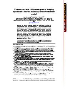
0.5-1.0 m 2 / g . Solar input was simulated with a cloud-free sky. To be able to analyze the impact of the phytoplankton specific absorption coefficient, a*ph , on the performance of the algorithms, as a first step, two data sets were simulated with the shapes of the specific absorption coefficient spectra taken, according to Eq. (2) from Ciotti et al. [26], as a sum of the specific absorptions coefficients of microplankton and picoplankton, as shown in Fig. 1. The weighting factor Sf ranged from 0.1 to 0.3. CNAP ranged from 0 to 1 mg/l in one data set and from 1 to 10 mg/l in the other data set. It should be noted that based on the dependence of a*ph (440) on [Chl], as shown in [27], the range 0-0.3 for Sf is typical for [Chl] > 1mg/m3. But we found that the model [26] usually underestimates a*ph values in the red and NIR parts of the spectrum [see Fig. 8(b) below]. For the purpose of evaluating the red–NIR models, we also used the spectral shapes from the model [26] in the 650-800 nm part of the spectrum with a*ph (675) = 0.0142, 0.0156, and 0.02 m2/(mg Chl a) which are also shown
in
Fig.
2
1.
For
the
spectral
shapes
with
a*ph (675)
=
0.0142
and
−1
0.02 m (mg Chl a) an additional set of IOP spectra and the associated reflectances was generated with CNAP = 0-10 mg/l, 1 < [Chl] < 40 mg/m3 (1 < [Chl] < 20 mg/m3 for a*ph (675) = 0.02 m2/(mg Chl a) and CDOM absorption at 400 nm, ay(400) = 0-3 m−1. This range of [Chl], 1 < [Chl] < 40 mg/m3, is more typical for coastal and inland waters (rather than higher [Chl] values). Thus, a very accurate evaluation of the algorithms is required for this [Chl] range. In all simulations the phytoplankton absorption was considered proportional to [Chl] #134029 - $15.00 USD
(C) 2010 OSA
Received 25 Aug 2010; revised 25 Oct 2010; accepted 26 Oct 2010; published 3 Nov 2010
8 November 2010 / Vol. 18, No. 23 / OPTICS EXPRESS 24112
a ph (λ ) = [Chl ]a*ph (λ )
(1)
* a*ph (λ ) = S f ⋅ a*pico (λ ) + (1 − S f ) ⋅ amicro (λ )
(2)
and
0.050 0.045
a*ph(675)= 0.02 m^2/(mg Chl a) a*ph(675)=0.0156 a*ph(675)=0.0142 a*ph(675)=0.0128 Sf=0.3 a*ph(675)=0.0114 Sf=0.2 a*ph(675)=0.01 Sf=0.1
a*ph, m2(mg Chl a)-1
0.040 0.035 0.030 0.025 0.020 0.015 0.010 0.005 0.000 -0.005 400
500
600
700
800
Wavelength, nm
Fig. 1. Phytoplankton specific absorption spectra used in the simulations.
Fluorescence quantum yield (together with the chlorophyll reabsorption coefficient) in the original simulations for Sf = 0.1-0.3 was, η = 0.5%. The fluorescence contribution was calculated as the difference between the total and elastic reflectances and was assumed to change proportionally with η, which enabled the assessment of the impact of the fluorescence component. All reflectances were simulated for the sun zenith angle θi = 30° and for nadir viewing. Field data set consisted of data collected by the CALMIT group at 85 stations in Fremont State Lakes, Nebraska, USA, during the summer of 2008, with [Chl] = 2-100 mg/m3, ay(400) = 0.9-3 m−1, and CNAP = 0-3 mg/l [28]. A standard set of water quality parameters was measured: turbidity, [Chl], total, inorganic, and organic suspended solids. Hyperspectral reflectance measurements were taken from a boat using two intercalibrated Ocean Optics USB2000 spectrometers. More details on the instrumentation and methodology are provided in Gitelson et al [28]. 3. Preliminary analysis of the main factors impacting red – NIR algorithms 3.1 Comparison of the synthetic and field data Moses et al. [29] calibrated and validated red-NIR models using MERIS satellite reflectances and [Chl] measured in the field. As a result of the calibration, the following linear relationships between [Chl] and the models were obtained. The two-band MERIS algorithm:
= [Chl]
61.324* Rrs (708) / Rrs (665) − 37.94
(3)
The three-band MERIS algorithm:
[Chl] =232.329[ (Rrs (665) −1 − Rrs (708) −1 ) *Rrs (753)] + 23.174
(4)
These relationships are compared in Fig. 2 with the relationships obtained between the models and [Chl] simulated from the synthetic data set for a*ph (675) = 0.0156 m2/(mg Chl a). As can be seen, for both two-band and three-band models, the relationships obtained from the
#134029 - $15.00 USD
(C) 2010 OSA
Received 25 Aug 2010; revised 25 Oct 2010; accepted 26 Oct 2010; published 3 Nov 2010
8 November 2010 / Vol. 18, No. 23 / OPTICS EXPRESS 24113
synthetic data set are closely related to those obtained from the field data set (RMSE = 4.05 mg/m3 and 5.58 mg/m3, respectively). Although further detailed analysis is required, especially for low [Chl] values, the close similarity of these relationships prompted the study of the sensitivity of the algorithms to variable water parameters. 120
120 a*ph =0.0156 0