Performance of recommender algorithms on top-n recommendation ...

Performance of Recommender Algorithms on Top-N Recommendation Tasks Paolo Cremonesi Politecnico di Milano Milan, Italy

[email protected]

Yehuda Koren

Roberto Turrin

[email protected]

[email protected]

Yahoo! Research Haifa, Israel

Neptuny Milan, Italy

ABSTRACT

General Terms

In many commercial systems, the ‘best bet’ recommendations are shown, but the predicted rating values are not. This is usually referred to as a top-N recommendation task, where the goal of the recommender system is to find a few specific items which are supposed to be most appealing to the user. Common methodologies based on error metrics (such as RMSE) are not a natural fit for evaluating the topN recommendation task. Rather, top-N performance can be directly measured by alternative methodologies based on accuracy metrics (such as precision/recall). An extensive evaluation of several state-of-the art recommender algorithms suggests that algorithms optimized for minimizing RMSE do not necessarily perform as expected in terms of top-N recommendation task. Results show that improvements in RMSE often do not translate into accuracy improvements. In particular, a naive non-personalized algorithm can outperform some common recommendation approaches and almost match the accuracy of sophisticated algorithms. Another finding is that the very few top popular items can skew the top-N performance. The analysis points out that when evaluating a recommender algorithm on the top-N recommendation task, the test set should be chosen carefully in order to not bias accuracy metrics towards nonpersonalized solutions. Finally, we offer practitioners new variants of two collaborative filtering algorithms that, regardless of their RMSE, significantly outperform other recommender algorithms in pursuing the top-N recommendation task, with offering additional practical advantages. This comes at surprise given the simplicity of these two methods.

Algorithms, Experimentation, Measurement, Performance

1.

Categories and Subject Descriptors H.3.4 [Information Storage and Retrieval]: Systems and Software—user profiles and alert services; performance evaluation (efficiency and effectiveness); H.3.3 [Information Storage and Retrieval]: Information Search and Retrieval— Information filtering

Permission to make digital or hard copies of all or part of this work for personal or classroom use is granted without fee provided that copies are not made or distributed for profit or commercial advantage and that copies bear this notice and the full citation on the first page. To copy otherwise, to republish, to post on servers or to redistribute to lists, requires prior specific permission and/or a fee. RecSys2010, September 26–30, 2010, Barcelona, Spain. Copyright 2010 ACM 978-1-60558-906-0/10/09 ...$10.00.

39

INTRODUCTION

A common practice with recommender systems is to evaluate their performance through error metrics such as RMSE (root mean squared error), which capture the average error between the actual ratings and the ratings predicted by the system. However, in many commercial systems only the ‘best bet’ recommendations are shown, while the predicted rating values are not [8]. That is, the system suggests a few specific items to the user that are likely to be very appealing to him. While the majority of the literature is focused on convenient error metrics (RMSE, MAE), such classical error criteria do not really measure top-N performance. At most, they can serve as proxies of the true top-N experience. Direct evaluation of top-N performance must be accomplished by means of alternative methodologies based on accuracy metrics (e.g., recall and precision). In this paper we evaluate – through accuracy metrics – the performance of several collaborative filtering algorithms in pursuing the top-N recommendation task. Evaluation is contrasted with performance of the same methods on the RMSE metric. Tests have been performed on the Netflix and Movielens datasets. The contribution of the work is threefold: (i) we show that there is no trivial relationship between error metrics and accuracy metrics; (ii) we propose a careful construction of the test set for not biasing accuracy metrics; (iii) we introduce new variants of existing algorithms that improve top-N performance together with other practical benefits. We first compare some state-of-the-art algorithms (e.g., Asymmetric SVD) with a non-personalized algorithm based on item popularity. The surprising result is that the performance of the non-personalized algorithm on top-N recommendations are comparable to the performance of sophisticated, personalized algorithms, regardless of their RMSE. However, a non-personalized, popularity-based algorithm can only provide trivial recommendations, interesting neither to users, which can get bored and disappointed by the recommender system, nor to content providers, which invest in a recommender system for pushing up sales of less known items. For such a reason, we run an additional set of experiments in order to evaluate the performance of the algorithms while excluding the extremely popular items. As expected, the accuracy of all algorithms decreases, as it is more difficult to recommend non-trivial items. Yet, ranking of the different algorithms aligns better with our expectations, with the

non-personalized methods being ranked lower. Thus, when evaluating algorithms in the top-N recommendation task, we would advise to carefully choose the test set, otherwise accuracy metrics are strongly biased. Finally, when pursuing a top-N recommendation task, exact rating prediction is not required. We present new variants of two collaborative filtering algorithms that are not designed for minimizing RMSE, but consistently outperform other recommender algorithms in top-N recommendations. This finding becomes even more important, when considering the simple and less conventional nature of the outperforming methods.

2.

100%

Netflix Movielens

% of items

10%

1%

0.1%

Short−head (popular)

Long−tail (unpopular)

0

TESTING METHODOLOGY

0

The testing methodology adopted in this study is similar to the one described in [6] and, in particular, in [10]. For each dataset, known ratings are split into two subsets: training set M and test set T . The test set T contains only 5-stars ratings. So we can reasonably state that T contains items relevant to the respective users. The detailed procedure used to create M and T from the Netflix dataset is similar to the one set for the Netflix prize, maintaining compatibility with results published in other research papers [3]. Netflix released a training dataset containing about 100M ratings, referred to as the training dataset. In addition to the training set, Netflix also provided a validation set, referred to as the probe set, containing 1.4M ratings. In this work, the training set M is the original Netflix training set, while the test set T contains all the 5-stars ratings from the probe set (|T |=384,573). As expected, the probe set was not used for training. We adopted a similar procedure for the Movielens dataset [13]. We randomly sub-sampled 1.4% of the ratings from the dataset in order to create a probe set. The training set M contains the remaining ratings. The test set T contains all the 5-star ratings from the probe set. In order to measure recall and precision, we first train the model over the ratings in M . Then, for each item i rated 5-stars by user u in T :

20%

40%

60%

% of ratings

80%

100%

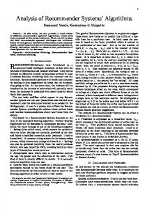
Figure 1: Rating distribution for Netflix (solid line) and Movielens (dashed line). Items are ordered according to popularity (most popular at the bottom). 0 or 1/N . The overall recall and precision are defined by averaging over all test cases: #hits |T | recall(N ) #hits precision(N ) = = N · |T | N recall(N ) =

where |T | is the number of test ratings. Note that the hypothesis that all the 1000 random items are non-relevant to user u tends to underestimate the computed recall and precision with respect to true recall and precision.

2.1

Popular items vs. long-tail

According to the well known long-tail distribution of rated items applicable to many commercial systems, the majority of ratings are condensed in a small fraction of the most popular items [1]. Figure 1 plots the empirical rating distributions of the Netflix and Movielens datasets. Items in the vertical axis are ordered according to their popularity, most popular at the bottom. We observe that about 33% of ratings collected by Netflix involve only the 1.7% of most popular items (i.e., 302 items). We refer to this small set of very popular items as the short-head, and to the remaining set of less popular items – about 98% of the total – as the long-tail [5]. We also note that Movielens’ rating distribution is slightly less long-tailed then Netflix’s: the short-head (33% of ratings) involves the 5.5% of popular items (i.e., 213 items). Recommending popular items is trivial and do not bring much benefits to users and content providers. On the other hand, recommending less known items adds novelty and serendipity to the users but it is usually a more difficult task. In this study we aim at evaluating the accuracy of recommender algorithms in suggesting non-trivial items. To this purpose, the test set T has been further partitioned into two subsets, Thead and Tlong , such that items in Thead are in the short-head while items in Tlong are in the long-tail of the distribution.

(i) We randomly select 1000 additional items unrated by user u. We may assume that most of them will not be of interest to user u. (ii) We predict the ratings for the test item i and for the additional 1000 items. (iii) We form a ranked list by ordering all the 1001 items according to their predicted ratings. Let p denote the rank of the test item i within this list. The best result corresponds to the case where the test item i precedes all the random items (i.e., p = 1). (iv) We form a top-N recommendation list by picking the N top ranked items from the list. If p ≤ N we have a hit (i.e., the test item i is recommended to the user). Otherwise we have a miss. Chances of hit increase with N . When N = 1001 we always have a hit. The computation of recall and precision proceeds as follows. For any single test case, we have a single relevant item (the tested item i). By definition, recall for a single test can assume either the value 0 (in case of miss) or 1 (in case of hit). Similarly, precision can assume either the value

3.

COLLABORATIVE ALGORITHMS

Most recommender systems are based on collaborative filtering (CF), where recommendations rely only on past user

40

nij sij where λ1 is a shrinking nij + λ1 factor [10]. A typical value of λ1 is 100. Neighborhood models are further enhanced by means of a kNN (k-nearest-neighborhood) approach. When predicting rating rui , we consider only the k items rated by u that are the most similar to i. We denote the set of most similar items by Dk (u; i). The kNN approach discards the items poorly correlated to the target item, thus decreasing noise for improving the quality of recommendations. Prior to comparing and summing different ratings, it is advised to remove different biases which mask the more fundamental relations between items. Such biases include itemeffects which represent the fact that certain items tend to receive higher ratings than others. They also include usereffects, which represent the tendency of certain users to rate higher than others. More delicate calculation of the biases, would also estimate temporal effects [11], but this is beyond the scope of this work. We take as baselines the static itemand user-biases, following [10]. Formally, the bias associated with the rating of user u to item i is denoted by bui . An item-item kNN method predicts the residual rating rui − bui as the weighted average of the residual ratings of similar items:

behavior (to be referred here as ‘ratings’, though such behavior can include other user activities on items like purchases, rentals and clicks), regardless of domain knowledge. There are two primary approaches to CF: (i) the neighborhood approach and (ii) the latent factor approach. Neighborhood models represent the most common approach to CF. They are based on the similarity among either users or items. For instance, two users are similar because they have rated similarly the same set of items. A dual concept of similarity can be defined among items. Latent factor approaches model users and items as vectors in the same ‘latent factor’ space by means of a reduced number of hidden factors. In such a space, users and items are directly comparable: the rating of user u on item i is predicted by the proximity (e.g., inner-product) between the related latent factor vectors.

3.1

as the coefficient dij =

Non-personalized models

Non-personalized recommenders present to any user a predefined, fixed list of items, regardless of his/her preferences. Such algorithms serve as baselines for the more complex personalized algorithms. A simple estimation rule, referred to as Movie Average (MovieAvg), recommends top-N items with the highest average rating. The rating of user u on item i is predicted as the mean rating expressed by the community on item i, regardless of the ratings given by u. A similar prediction schema, denoted by Top Popular (TopPop), recommends top-N items with the highest popularity (largest number of ratings). Notice that in this case the rating of user u about item i cannot be inferred, but the output of this algorithm is only a ranked list of items. As a consequence, RMSE or other error metrics are not applicable.

3.2

rˆui = bui +

P

j∈D k (u;i)

P

dij (ruj − buj )

j∈D k (u;i)

dij

(1)

Hereinafter, we refer to this model as Correlation Neighborhood (CorNgbr), where sij is measured as the Pearson correlation coefficient.

3.2.1

Non-normalized Cosine Neighborhood

Notice that in (1), the denominator forces that predicted rating values fall in the correct range, e.g., [1 . . . 5] for a typical star-ratings systems. However, for a top-N recommendation task, exact rating values are not necessary. We simply want to rank items by their appeal to the user. In such a case, we can simplify the formula by removing the denominator. A benefit of this would be higher ranking for items P with many similar neighbors (that is high j∈D k (u;i) dij ), where we have a higher confidence in the recommendation. Therefore, we propose to rank items by the following coefficient denoted by rˆui : X rˆui = bui + dij (ruj − buj ) (2)

Neighborhood models

Neighborhood models base their prediction on the similarity relationships among either users or items. Algorithms centered on user-user similarity predict the rating by a user based on the ratings expressed by users similar to him about such item. On the other hand, algorithms centered on item-item similarity compute the user preference for an item based on his/her own ratings on similar items. The latter is usually the preferred approach (e.g., [15]), as it usually performs better in RMSE terms, while being more scalable. Both advantages are related to the fact that the number of items is typically smaller than the number of users. Another advantage of item-item algorithms is that reasoning behind a recommendation to a specific user can be explained in terms of the items previously rated by him/her. In addition, basing the system parameters on items (rather than users) allows aseamless handling of users and ratings new to the system. For such reasons, we focus on item-item neighborhood algorithms. The similarity between item i and item j is measured as the tendency of users to rate items i and j similarly. It is typically based either on the cosine, the adjusted cosine, or (most commonly) the Pearson correlation coefficient [15]. Item-item similarity is computed on the common raters. In the typical case of a very sparse dataset, it is likely that some pairs of items have a poor support, leading to a nonreliable similarity measure. For such a reason, if nij denotes the number of common raters and sij the similarity between item i and item j, we can define the shrunk similarity dij

j∈D k (u;i)

Here rˆui does not represent a proper rating, but is rather a metric for the association between user u and item i. We should note that similar non-normalized neighborhood rules were mentioned by others [7, 10]. In our experiments, the best results in terms of accuracy metrics have been obtained by computing sij as the cosine similarity. Unlike Pearson correlation which is computed only on ratings shared by common raters, the cosine coefficient between items i and j is computed over all ratings (taking missing values as zeroes), that is: cos(i, j) = ~i ·~j/(||~i|| ·||~j|| ). We denote such model by Non-Normalized 2 2 Cosine Neighborhood (NNCosNgbr).

3.3

Latent Factor Models

Recently, several recommender algorithms based on latent factor models have been proposed. Most of them are

41

Dataset Users Items Ratings Density Movielens 6,040 3,883 1M 4.26% Netflix 480,189 17,770 100M 1.18%

based on factoring the user-item ratings matrix [12], also informally known as SVD models after the related Singular Value Decomposition. The key idea of SVD models is to factorize the user-item rating matrix to a product of two lower rank matrices, one containing the so-called ‘user factors’, while the other one containing the so-called ‘item-factors’. Thus, each user u is represented with an f -dimensional user factors vector pu ∈ ℜf . Similarly, each item i is represented with an item factors vector qi ∈ ℜf . Prediction of a rating given by user u for item i is computed as the inner product between the related factor vectors (adjusted for biases), i.e., rˆui = bui + pu qi T

Table 1: Statistical properties of Movielens and Netflix. orthonormal matrix, and Σ is a f × f diagonal matrix containing the first f singular values. In order to demonstrate the ease of imputing zeroes, we should mention that we used a non-multithreaded SVD package (SVDLIBC, based on the SVDPACKC library [4]), which factorized the 480K users by 17,770 movies Netflix dataset under 10 minutes on an i7 PC (f = 150). Let us define P = U · Σ, so that the u-th row of P represents the user factors vector pu , while the i-th row of Q represents the item factors vector qi . Accordingly, rˆui can be computed similarly to (3). In addition, since U and Q have orthonormal columns, we can straightforwardly derive that:

(3)

Since conventional SVD is undefined in the presence of unknown values – i.e., the missing ratings – several solutions have been proposed. Earlier works addressed the issue by filling missing ratings with a baseline estimations (e.g., [16]). However, this leads to a very large, dense user rating matrix, whose factorization becomes computationally infeasible. More recent works learn factor vectors directly on known ratings through a suitable objective function which minimizes prediction error. The proposed objective functions are usually regularized in order to avoid overfitting (e.g., [14]). Typically, gradient descent is applied to minimize the objective function. As with neighborhood methods, this article concentrates on methods which represent users as a combination of item features, without requiring any user-specific parameterization. The advantages of these methods are that they can create recommendations for users new to the system without re-evaluation of parameters. Likely, they can immediately adjust their recommendations to just entered ratings, providing users with an immediate feedback for their actions. Finally, such methods can explain their recommendations in terms of items previously rated by the user. Thus, we experimented with a powerful matrix factorization model, which indeed represents users as a combination of item features. The method is known as Asymmetric-SVD (AsySVD) and is reported to reach an RMSE of 0.9000 on the Netflix dataset [10]. In addition, we have experimented with a beefed up matrixfactorization approach known as SVD++ [10], which represents highest quality in RMSE-optimized factorization methods, albeit users are no longer represented as a combination of item features; see [10].

3.3.1

P=U·Σ=R·Q

where R is the user rating matrix. Consequently, by denoting with ru the u-th row of the user rating matrix - i.e., the vector of ratings of user u, we can rewrite the prediction rule rˆui = ru · Q · qi T

(6)

Note that, similarly to (1), in a slight abuse of notation, the symbol rˆui , is not exactly a valid rating value, but an association measure between user u and item i. In the following we will refer to this model as PureSVD. As with item-item kNN and AsySVD, PureSVD offers all the benefits of representing users as a combination of item features (by Eq. (5)), without any user-specific parameterization. It also offers convenient optimization, which does not require tunning learning constants.

4.

RESULTS

In this section we present the quality of the recommender algorithms presented in Section 3 on two standard datasets: MovieLens [13] and Netflix [3]. Both are publicly available movie rating datasets. Collected ratings are in a 1-to-5 star scale. Table 1 summarizes their statistical properties. We used the methodology defined in Section 2 for evaluating six recommender algorithms. The first two - MovieAvg and TopPop - are non-personalized algorithms, and we would expect them to be outperformed by any recommender algorithm. The third prediction rule - CorNgbr - is a well tuned neighborhood-based algorithm, probably the most popular in the literature of collaborative filtering. The forth algorithm is a variant of CorNgbr - NNCosNgbr - and it is one of the two proposed algorithm oriented to accuracy metrics. Fifth is the latent factor model AsySVD with 200 factors. Sixth is a 200-D SVD++, among the most powerful latent factor models in terms of RMSE. Finally, we consider our variant of latent factor models, PureSVD, which is shown in two configurations: one with a fewer latent factors (50), and one with a larger number of latent factors (150 for Movielens and 300 for the larger Netflix dataset). Three of the algorithms – TopPop, NNCosNgbr, and PureSVD – are not sensible from an error minimization viewpoint and cannot be assessed by an RMSE measure. The other four

PureSVD

While pursuing a top-N recommendation task, we are interested only in a correct item ranking, not caring about exact rating prediction. This grants us some flexibility, like considering all missing values in the user rating matrix as zeros, despite being out of the 1-to-5 star rating range. In terms of predictive power, the choice of zero is not very important, and we have received similar results with higher imputed values. Importantly, now we can leverage existing highly optimized software packages for performing conventional SVD on sparse matrices, which becomes feasible since all matrix entries are now non-missing. Thus, the user rating matrix R is estimated by the factorization [2]: ˆ = U · Σ · QT R

(5)

(4)

where, U is a n × f orthonormal matrix, Q is a m × f

42

algorithms were optimized to deliver best RMSE results, and their RMSE scores on the Netflix test set are as follows: 1.053 for MovieAvg, 0.9406 for CorNgbr, 0.9000 for AsySVD, and 0.8911 for SVD++ [10]. For each dataset, we have performed one set of experiments on the full test set and one set of experiments on the long-tail test set. We report the recall as a function of N (i.e., the number of items recommended), and the precision as a function of the recall. As for recall(N ), we have zoomed in on N in the range [1 . . . 20]. Larger values of N can be ignored for a typical top-N recommendations task. Indeed, there is no difference whether an appealing movie is placed within the top 100 or the top 200, because in neither case it will be presented to the user.

4.1

ures 4 and 5 show the performance of the algorithms on the Netflix dataset. As before, we focus on both the full test set and the long-tail test set. Once again, non-personalized TopPop shows surprisingly good results when including the 2% head items, outperforming the widely popular CorNgbr. However, the more powerful AsySVD and SDV++, which were possibly better tuned for the Netflix data, are slightly outperforming TopPop. Note also that AsySVD is now in line with SVD++. Consistent with the Movielens experience, the best performing algorithm in terms of recall and precision is still the non-RMSE-oriented PureSVD. As for the other non-RMSEoriented NNCosNgbr, the picture becomes mixed. It is still outperforming the RMSE-oriented algorithms when including the head items, but somewhat underperforms them when the top-2% most popular items are excluded. The behavior of the commonly used CorNgbr on the Netflix dataset is very surprising. While it significantly underperforms others on the full test set, it becomes among the top-performers when concentrating on the longer tail. In fact, while all the algorithms decrease their precision and recall when passing from the full to the long-item test set, CorNgbr appears more accurate in recommending long-tail items. After all, the wide acceptance of the CorNgbr approach might be for a reason given the importance of longtail items.

Movielens dataset

Figure 2 reports the performance of the algorithms on the Movielens dataset over the full test set. It is apparent that the algorithms have significant performance disparity in terms of top-N accuracy. For instance, the recall of AsySVD at N = 10 is about 0.28, i.e., the model has a probability of 28% to place an appealing movie in the top-10. Surprisingly, the recall of the non-personalized TopPop is very similar to AsySVD (e.g., at N = 10 recall is about 0.29). The best algorithms in terms of accuracy are the non-RMSE-oriented NNCosNgbr and PureSVD, which reach, at N = 10, a recall equaling about 0.44 and 0.52, respectively. As for the latter, this means that about 50% of 5-star movies are presented in a top-10 recommendation. The best algorithm in the RMSE-oriented familiy is SVD++, with a recall close to that of NNCosNgbr. Figure 2(b) confirms that PureSVD also outperforms the other algorithms in terms of precision metrics, followed by the other non-RMSE-oriented algorithm – NNCosNgbr. Each line represents the precision of the algorithm at a given recall. For example, when the recall is about 0.2, precision of NNCosNgbr is about 0.12. Again, TopPop performance is aligned with that of a state-of-the-art algorithm as AsySVD. We should note the gross underperformance of the widely used CorNgbr algorithm, whose performance is in line with the very naive MovieAvg. We should also note that the precision of SVD++ is competitive with that of PureSVD50 for small values of recall. The strange and somehow unexpected result of TopPop motivates the second set of experiments, accomplished over the long-tail items, whose results are drawn in Figure 3. As a reminder, now we exclude the very popular items from consideration. Here the ordering among the several recommender algorithms better aligns with our expectations. In fact, recall and precision of the non-personalized TopPop dramatically falls down and it is very unlikely to recommend a 5-star movie within the first 20 positions. However, even when focusing on the long-tail, the best algorithms is still PureSVD, whose recall at N = 10 is about 40%. Note that while the best performance of PureSVD was with 50 latent factors in the case of full test set, here the best performance is reached with a larger number of latent factors, i.e., 150. Performance of NNCosNgbr now becomes significantly worse than PureSVD, while SVD++ is the best within the RMSE-oriented algorithms.

4.2

5.

DISCUSSION — PureSVD

Over both Movielens and Netflix datasets, regardless of inclusion of head-items, PureSVD is consistently the top performer, beating more detailed and sophisticated latent factor models. Given its simplicity, and poor design in terms of RMSE optimization, we did not expect this result. In fact, we would view it as a good news for practitioners of recommender systems, as PureSVD combines multiple advantages. First, it is very easy to code, without a need to tune learning constants, and fully relies on off-the-shelf optimized SVD packages . This comes with good computational performance in both offline and online modes. PureSVD also has the convenience of representing the users as a combination of item features (Eq. (6)), offering designers a flexibility in handling new users, new ratings by existing users and explaining the reasoning behind the generated recommendations. An interesting finding, observed at both Movielens and Netflix datasets, is that when moving to longer tail items, accuracy improves with raising the dimensionality of the PureSVD model. This may be related to the fact that the first latent factors of PureSVD capture properties of the most popular items, while the additional latent factors represent more refined features related to unpopular items. Hence, when practitioners use PureSVD, they should pick its dimensionality while accounting for the fact that the number of latent factors influences the quality of long-tail items differently than head items. We would like to offer an explanation as to why PureSVD could consistently deliver better top-N results than best RMSErefined latent factor models. This may have to do with a limitation of RMSE testing, which concentrates only on the ratings that the user provided to the system. This way, RMSE (or MAE for the matter) is measured on a held-out test set containing only items that the user chose to rate, while completely missing any evaluation of the method on

Netflix dataset

Analogously to the results presented for Movielens, Fig-

43

0.7 0.6

0.12

0.08

0.4 0.3

0.06

0.04

0.2

0.02

0.1 0 0

MovieAvg TopPop CorNgbr NNCosNgbr AsySVD SVD++ PureSVD50 PureSVD150

0.1

precision

recall(N)

0.5

MovieAvg TopPop CorNgbr NNCosNgbr AsySVD SVD++ PureSVD50 PureSVD150

5

10

N

15

0 0

20

0.2

(a) recall

0.4

recall

0.6

0.8

1

(b) precision vs recall

Figure 2: Movielens: (a) recall-at-N and (b) precision-versus-recall on all items.

0.6

recall(N)

0.5 0.4

0.07 MovieAvg TopPop CorNgbr NNCosNgbr AsySVD SVD++ PureSVD50 PureSVD150

0.05

0.3

0.04 0.03

0.2

0.02

0.1

0.01

0 0

5

MovieAvg TopPop CorNgbr NNCosNgbr AsySVD SVD++ PureSVD50 PureSVD150

0.06

precision

0.7

10

N

15

0 0

20

(a) recall

0.2

0.4

recall

0.6

0.8

1

(b) precision vs recall

Figure 3: Movielens: (a) recall-at-N and (b) precision-versus-recall on long-tail (94% of items).

44

0.7 0.6

0.1

MovieAvg TopPop CorNgbr NNCosNgbr AsySVD SVD++ PureSVD50 PureSVD300

0.09 0.08 0.07

0.4

precision

recall(N)

0.5

MovieAvg TopPop CorNgbr NNCosNgbr AsySVD SVD++ PureSVD50 PureSVD300

0.3 0.2

0.06 0.05 0.04 0.03 0.02

0.1

0.01 0 0

5

10

N

15

0 0

20

0.2

(a) recall

0.4

recall

0.6

0.8

1

(b) precision vs recall

Figure 4: Netflix: (a) recall-at-N and (b) precision-versus-recall on all items.

0.7 0.6

0.08

0.06

0.4 0.3 0.2

0.05 0.04 0.03 0.02

0.1 0 0

MovieAvg TopPop CorNgbr NNCosNgbr AsySVD SVD++ PureSVD50 PureSVD300

0.07

precision

recall(N)

0.5

MovieAvg TopPop CorNgbr NNCosNgbr AsySVD SVD++ PureSVD50 PureSVD300

0.01 5

10

N

15

0 0

20

(a) recall

0.2

0.4

recall

0.6

0.8

1

(b) precision vs recall

Figure 5: Netflix: (a) recall-at-N and (b) precision-versus-recall on long-tail (98% of items).

45

items that the user has never rated. This testing-mode bodes well with the RMSE-oriented models, which are trained only on the known ratings, while largely ignoring the missing entries. Yet, such a testing methodology misses much of the reality, where all items should count, not only those actually rated by the user in the past. The proposed Top-N based accuracy measures indeed do better in this respect, by directly involving all possible items (including unrated ones) in the testing phase. This may explain the outperformance of PureSVD, which considers all possible user-item pairs (regardless of rating availability) in the training phase. Our general advise to practitioners is to consider PureSVD as a recommender algorithm. Still there are several unexplored ways that may improve PureSVD. First, one can optimize the value imputed at the missing entries. Direct usage of ready sparse SVD solvers (which usually assume a default value of zero) would still be possible by translating all given scores. For example, imputing a value of 3 instead of zero would be effectively achieved by translating the given star ratings from the [1...5] range into the [-2...2] range. Second, one can grant a lower confidence to the imputed values, such that SVD will emphasize more efforts on real ratings. For an explanation on how this can be accomplished consider [9]. However, we would expect such a confidence weighting to significantly increase the time complexity of the offline training.

6.

[2] R. Bambini, P. Cremonesi, and R. Turrin. Recommender Systems Handbook, chapter A Recommender System for an IPTV Service Provider: a Real Large-Scale Production Environment. Springer, 2010. [3] J. Bennett and S. Lanning. The Netflix Prize. Proceedings of KDD Cup and Workshop, pages 3–6, 2007. [4] M. W. Berry. Large-scale sparse singular value computations. The International Journal of Supercomputer Applications, 6(1):13–49, Spring 1992. [5] O. Celma and P. Cano. From hits to niches? or how popular artists can bias music recommendation and discovery. Las Vegas, USA, August 2008. [6] P. Cremonesi, E. Lentini, M. Matteucci, and R. Turrin. An evaluation methodology for recommender systems. 4th Int. Conf. on Automated Solutions for Cross Media Content and Multi-channel Distribution, pages 224–231, Nov 2008. [7] M. Deshpande and G. Karypis. Item-based top-n recommendation algorithms. ACM Transactions on Information Systems (TOIS), 22(1):143–177, 2004. [8] J. Herlocker, J. Konstan, L. Terveen, and J. Riedl. Evaluating collaborative filtering recommender systems. ACM Transactions on Information Systems (TOIS), 22(1):5–53, 2004. [9] Y. Hu, Y. Koren, and C. Volinsky. Collaborative filtering for implicit feedback datasets. Data Mining, IEEE International Conference on, 0:263–272, 2008. [10] Y. Koren. Factorization meets the neighborhood: a multifaceted collaborative filtering model. In KDD ’08: Proceeding of the 14th ACM SIGKDD international conference on Knowledge discovery and data mining, pages 426–434, New York, NY, USA, 2008. ACM. [11] Y. Koren. Collaborative filtering with temporal dynamics. In KDD ’09: Proceedings of the 15th ACM SIGKDD international conference on Knowledge discovery and data mining, pages 447–456, New York, NY, USA, 2009. ACM. [12] Y. Koren, R. M. Bell, and C. Volinsky. Matrix factorization techniques for recommender systems. IEEE Computer, 42(8):30–37, 2009. [13] B. Miller, I. Albert, S. Lam, J. Konstan, and J. Riedl. MovieLens unplugged: experiences with an occasionally connected recommender system. Proceedings of the 8th international conference on Intelligent user interfaces, pages 263–266, 2003. [14] A. Paterek. Improving regularized singular value decomposition for collaborative filtering. Proceedings of KDD Cup and Workshop, 2007. [15] B. Sarwar, G. Karypis, J. Konstan, and J. Reidl. Item-based collaborative filtering recommendation algorithms. 10th Int. Conf. on World Wide Web, pages 285–295, 2001. [16] B. Sarwar, G. Karypis, J. Konstan, and J. Riedl. Application of Dimensionality Reduction in Recommender System-A Case Study. Defense Technical Information Center, 2000.

CONCLUSIONS

Evaluation of recommender has long been divided between accuracy metrics (e.g., precision/recall) and error metrics (notably, RMSE and MAE). The mathematical convenience and fitness with formal optimization methods, have made error metrics like RMSE more popular, and they are indeed dominating the literature. However, it is well recognized that accuracy measures may be a more natural yardstick, as they directly assess the quality of top-N recommendations. This work shows, through an extensive empirical study, that the convenient assumption that an error metric such as RMSE can serve as good proxy for top-N accuracy is questionable at best. There is no monotonic relation between error metrics and accuracy metrics. This may call for a reevaluation of optimization goals for top-N systems. On the bright side we have presented simple and efficient variants of known algorithms, which are useless in RMSE terms, and yet deliver superior results when pursuing top-N accuracy. In passing, we have also discussed possible pitfalls in the design of a test set for conducting a top-N accuracy evaluation. In particular, a careless construction of the test set would make recall and precision strongly biased towards non personalized algorithms. An easy solution, which we adopted, was excluding the extremely popular items from the test set (while retaining ∼98% of the items). The resulting test set, which emphasizes the rather important nontrivial items, seems to shape better with our expectations. First, it correctly shows the lower value of non-personalized algorithms. Second, it shows a good behavior for the widely used correlation-based kNN approach, which otherwise (when evaluated on the full set of items) exhibits extremely poor results, strongly confronting the accepted practice.

7.

REFERENCES

[1] C. Anderson. The Long Tail: Why the Future of Business Is Selling Less of More. Hyperion, July 2006.

46