Performance of the Effective-characteristic-polynomial Π2 Method for Diatomic Molecules: Basis-set Dependencies and Vibrational Levels Herbert H. H.Homeier and M. D. Neef Email:
[email protected] Institut f¨ ur Physikalische und Theoretische Chemie Universit¨at Regensburg D-93040 Regensburg, Germany October 19, 1999 Abstract The performance of the recently introduced Π2 method [1] is investigated for some diatomic molecules. For this end, ground state energies are calculated at the MP4 level for various basis sets of increasing size. With negligible extra effort, the Π2, F4, and [2/2] estimators are obtained, together with information on the reliability of the basic perturbation series [1]. The results are compared to more expensive CCSD(T) results. Also, electronic energy hypersurfaces are calculated at these levels. As a further possibility to test the performance of the method, vibrational frequencies and other spectroscopic constants of diatomic molecules are calculated by fitting different analytic functions to the hypersurfaces obtained by different methods and compared to experimental data. [1] H. H. H. Homeier, Correlation energy estimators based on Møller-Plesset perturbation theory, J. Mol. Struct. (Theochem), 366:161-171, 1996. Category: Ab initio Keywords: Correlation energy, Perturbation theory, Morse potential, Anharmonicity constant, Hypersurface, Spectroscopic constants
1
Introduction
Recently, methods have been discussed for the computation of correlation energy estimators based on Møller-Plesset (MP) perturbation theory that may also be regarded as accelerating the convergence of the MP series [1],[2],[3],[4],[5],[6],[7],[8],[9],[10]. In [8], some methods were discussed that are based on MP calculations of fourth order (MP4)1 : • The Feenberg energy of fourth order F4 [11],[12],[10],[8], • The Pad´e approximant [2/2]2 , [13],[14],[15] • The Π2 approximation that is computed as the zero of an effective characteristic polynomial [16],[17],[18],[19],[20],[21],[22],[23] of degree 2. All these approximations are calculated from the terms of the MP series with negligible extra effort. Explicit formulas for these methods are given in Section 2. All the methods are sizeextensive [8],[9]. Also, test calculations were reported in [8] for a rather large number of small molecules (BH, HF, CH2 , H2 O, NH2 , NH3 , CO, C2 H2 , O3 , CN) for which Full Configuration Interaction (FCI) or Coupled-Cluster (CC) including Single (S), Double (D) and Triple (T) excitations, i.e., CCSDT results are available, mainly for basis sets of double zeta (DZ) or DZ plus polarization (DZP) quality. It was shown that (for the treated cases) the Π2 method yields very good approximations for the energy if the values of F4, [2/2] and Π2 are sufficiently close together. If the latter criterion is satisfied, all three methods improve the MP4 values considerably. The above criterion to accept the result of the perturbation calculation is especially important since it is well-known that the quality of the MP results deteriorates for greater distances from the equilibrium geometry. Thus, the criterion allows to judge the quality of the MP series. The criterion will be further discussed in Section 2. In the present contribution, we report further studies of the performance of the Π2 and also the F4 and [2/2] methods. In particular, the dependence on the choice of the basis sets is important for the application of the methods. We limit attention to diatomic systems. Also, we report some results concerning the quality of potential energy surfaces and the calculation of spectroscopic constants.
2
Methods
The ab initio MP4 and CCSD(T) calculations were done using the Gaussian 94 program package [24]. For all systems under study, we calculate properties of the lowest singlet state. For the MP energy terms, we used (1) E2 = E(M P 2) − E(SCF ), E3 = E(M P 3) − E(M P 2), E4 = E(M P 4SDT Q) − E(M P 3). Then, the F4 energy is given by (2)
F 4 = E(SCF ) + 3
E23 (−E2 + 2 E3 − E4) (−E2 + E3)
3
constants three different approaches were examined. Two fits of a narrow region around the minimum by polynomials of degree 3 or 5 were used to calculate the five spectroscopic constants ωe , ωe xe , Be , αe , De , the equilibrium distance Re , the force constant k e and the minimum total electronic energy U e . The third approach using a four parameter Morse potential as fit function yielded the two constants ωe and ωe xe . The calculated spectroscopic constants arise from a second order approximation of the rovibrational energy as follows: (7)
Etot (v, J) = Evib (v) + Erot (v, J)
with (8)
1 1 Evib (v) = ωe (v + ) − ωe xe (v + )2 2 2
and (9)
Erot (v, J) = Bv J(J + 1) − Dv J 2 (J + 1)2
where (10)
1 Bv = Be − αe (v + ) 2
and (11)
1 Dv = De + βe (v + ). 2 The centrifugal distortion constant De should not be confused neither with the dissociation energy D0 nor the depth De of the potential at the minimum. The Morse data were obtained by a least square fit of a Morse potential U (R) = U e + De (1 − exp(−β(R − Re )))2
(12)
with fit parameters U e , De , Re , β to a suitable part of the calculated potential surface that was chosen according to the above criterion (6). A Fortran 77 program which used the NAG [26] routine E04FDF was used in the fitting procedure. We follow the spectroscopic praxis and choose cm−1 as unit for energies and frequencies in formulas and tables. The vibrational frequency ω e and the first anharmonicity constant were then calculated from the parameters of the Morse potential using the formulas √ ~De ωe = β (13) πcµ and (14)
ω e xe =
ω 2e 4De
where µ is the reduced mass of the diatomic molecule. The least square fitting of the polynomials to the potential curves was done using a MapleV [27] worksheet in each case. From the coefficients Re ,k e ,a,b of the fitted polynomial (15)
U (x) = U e +
ke (x − Re )2 − a(x − Re )3 + b(x − Re )4 + c(x − Re )5 2
the spectroscopic constants were calculated in the following way [28], chapter 1.4
√
(16)
1 ωe = 2πc
(17)
Be =
(18)
αe = 24
(19)
ω e xe =
~ 4πcµR2e
a(B e Re )3 B 2e − 6 ω 3e ωe
30B 3e R6e a2 6B 2e R4e b − ω 4e ω 2e De =
(20)
ke µ
4B 3e ω 2e
In the case of a polynom fit of third degree we set b = 0 and c = 0.
3 3.1
Results and Discussion Single-point Calculations
Using the methods described in Section 2, single-point calculations were done for various diatomic systems in the vicinity of the equilibrium geometry using basis sets of varying sizes. In the table below we compare the relative quality of full core and frozen core results with the validity of criterion (6) averaged over the different basis sets. For each molecule except Hydrogen we
3.2
Potential Energy Surfaces and Spectroscopical Parameters
In Figures 2, 3, 4, and 5, the potential energy surface of LiH is shown as computed with different basis sets. For each basis set, MP4, F4, [2/2], Π2 and CCSD(T) results are presented. In this particular example, the Π2 methods is closest to the CCSD(T) result up to R ≈ 5 bohr where the criterion (6) is satisfied. For larger distances R, this is no longer the case, and in the case of Figures 2 and 4, some unphysical behavior of the Π2 surface is seen in this region where however the criterion (6) indicates that the perturbative results are not acceptable. Comparing the figures, it is also observed that in this case, adding polarization functions slightly enlarges the region where the criterion is satisfied, while adding diffuse functions does not have a large effect. In order to further judge the quality of the method, a Morse potential and polynomials of degree 3 and 5 were fitted to the data as described in Section 2. The results are displayed in Tables 18 to 22 and Figures 6 (LiH), 7 (HF), 8 (HCl) and 9 (N2 ). The color code is blue for MP4, red for Π2, and green for CCSD(T) results. Broken lines represent Morse fits, and full lines the polynomial fit of third degree to the data points that are displayed also. It is seen that in the equilibrium region, the Morse fits often are lying below the data although they reproduce the overall shape of the curves nicely. This leads to the assumption that the vibrational parameters will be acceptable for the Morse fit. The third degree polynomial fits are in most cases more accurate in the region of the minimum but differ significantly from the potential curve for bigger distances. Hence, it is expected that they will produce more accurate estimates for the harmonic frequencies but worse values for the other spectroscopic constants which should be calculated using a 5th degree fitting polynomial. This is indeed the case. In Table 18 we report the results for the harmonic frequencies, the anharmonic correction term obtained from the Morse fit, the values of the resulting fit parameters De and β and experimental data from Refs. [29] and (in parentheses) [30]. The results for the polynomial fits, 8 Parameter for each molecule, are shown in Tables 19 (LiH),20 (HF), 21 (HCl) and 22 (N2 ). In this context, it should be noted that all results are relatively sensitive to the selection of the data points used in the fitting procedure. In the fits, we usually included all points that are compatible with the criterion (6) in case of the Morse potential – beware that not all these data points are displayed in the figures in order to be able to simultaneously display the Morse and polynomial fits with sufficient resolution –, and 8 points around the minimum for the polynomial fit. The selection of the latter points is plain from the corresponding figures. In the case of N2 , the MP4 values for R > 2.6 bohr were unphysical and excluded from the fit. Also, the criterion (6) was not satisfied in this region. However, since it was observed that the Π2 results agreed rather closely the CCSD(T) results even in this region, we included some points from this region also in order to produce the corresponding Morse fits. The results for the harmonic frequency as obtained from a second Morse fit using only points for which the criterion (6) was satisfied was close to the result displayed in Table 18 while the value for the anharmonicity constant was worse. The main results using Π2/6 − 311G and CCSD(T )/6 − 311G levels of theory are that • the Π2 results are sufficiently close to the (more expensive) CCSD(T) method using the same fit methodology, • harmonic frequencies are in most cases better (accuracy 1-3 percent) calculated via polynomial fits of third degree than using Morse fits that can be competitive if these fits of the potential surface are in the equilibrium region of high accuracy, as in the case of the HF molecule, or at least have the same shape as the polynomial fit, as in the case of LiH, • Morse fits are able to reproduce experimental anharmonic parameter xe with an accuracy of about 10-30 percent. For this parameter the 5th degree polynomial fit results are of similar accuracy whereas for the remaining three spectroscopic constants the accuracy lies around 5-10 percent.
3.3
Conclusion
In conclusion, the Π2 method is seen to perform similarly to the more expensive CCSD(T) method if the criterion (6) is satisfied. This is equally valid for frozen and full core calculations. Especially for ”difficult” molecules like N2 the quality of the calculated spectroscopic constants can be improved significantly using the Π2 method instead of MP4. For DZ- and DZP-quality basis sets, usually good results are obtained whereas adding diffuse functions does not always yield an improvement for the quality of the perturbational methods.
4
Acknowledgement
Financial support of the Deutsche Forschungsgemeinschaft in the project Die Berechnung der Energiezust¨ ande von Quantensystemen mittels effektiver charakteristischer Polynome auf der Grundlage von St¨ orungsreihen and the Verein der Freunde der Universit¨ at Regensburg e.V. is gratefully acknowledged. H.H.H.H. also acknowledges financial support by the Fonds der Chemischen Industrie.
5
Tables
For detailed explanations of the meaning of the following data see Sec. 3.1.
Basis 3-21G 4-31G 6-31G 6-311G 6-311G(d,p) 6-311G(3df,2p) 6-311++G Dunning DZ Dunning DZP Dunning DZP+diff Dunning TZ cc-p-VDZ cc-p-VTZ AUG cc-p-VDZ
MP4 -48.751134 -48.953405 -49.013358 -49.064917 -49.113682 -49.152838 -49.066636 -49.044619 -49.082232 -49.083394 -49.063643 -49.072115 -49.121360 -49.080497
F4 -48.759092 -48.960828 -49.021379 -49.072378 -49.120836 -49.158225 -49.074051 -49.052475 -49.089432 -49.090541 -49.071194 -49.080373 -49.126569 -49.088505
[2/2] -48.766450 -48.969685 -49.029569 -49.078850 -49.127568 -49.164410 -49.080497 -49.056773 -49.094560 -49.095783 -49.077818 -49.087292 -49.133500 -49.094912
Π2 -48.829253 -49.051426 -49.106974 -49.113003 -49.156699 -49.184867 -49.114295 -49.082403 -49.119004 -49.120513 -49.114272 -49.126796 -49.157880 -49.128833
Table 1: B2 , R=3.13 bohr, full core CCSD(T) -48.742630 -48.945615 -49.583559 -49.665516 -49.102234 -49.139593 -49.670688 -49.036684 -49.787531 -49.786059 -49.661605 -49.727998 -49.108293 -49.727220
Basis 3-21G 4-31G 6-31G 6-311G 6-311G(d,p) 6-311G(3df,2p) 6-311++G Dunning DZ Dunning DZP Dunning DZP+diff Dunning TZ cc-p-VDZ cc-p-VTZ AUG cc-p-VDZ AUG cc-p-VTZ
MP4 -48.748966 -48.950762 -49.011157 -49.030472 -49.076451 -49.096937 -49.031991 -49.017109 -49.052655 -49.053692 -49.033240 -49.067474 -49.097514 -49.072671 -49.099559
F4 -48.757182 -48.958444 -49.019430 -49.037706 -49.083318 -49.101448 -49.039172 -49.024893 -49.059479 -49.060446 -49.040383 -49.076090 -49.102643 -49.081069 -49.104305
[2/2] -48.764715 -48.967563 -49.027829 -49.046694 -49.092077 -49.109735 -49.048128 -49.030785 -49.066122 -49.067223 -49.049218 -49.083259 -49.110571 -49.087874 -49.112014
Π2 -48.839818 -49.077452 -49.139437 -49.158408 -49.138885 -49.140053 -49.148217 -49.073897 -49.101248 -49.102837 -49.139848 -49.127627 -49.141289 -49.127420 -49.140237
Table 2: B2 , R=3.13 bohr, frozen core CCSD(T) -48.740443 -48.942960 -49.003115 -49.600385 -49.742210 -49.083486 -49.605121 -49.009149 -49.042690 -49.043625 -49.609209 -49.056230 -49.739408 -49.713183 -49.086344
For detailed explanations of the meaning of the following data see Sec. 3.2.
Basis 3-21G 4-31G 6-31G 6-311G 6-311G(d,p) 6-311G(3df,2p) 6-311++G Dunning DZ Dunning DZP
MP4 -25.033956 -25.135758 -25.167247 -25.194634 -25.233940 -25.251448 -25.195699 -25.182810 -25.216566
F4 -25.038944 -25.141305 -25.172614 -25.198815 -25.237485 -25.254632 -25.199840 -25.187302 -25.220145
[2/2] -25.037724 -25.139923 -25.171317 -25.197736 -25.236603 -25.253814 -25.198772 -25.186184 -25.219254
Π2 -25.039643 -25.142173 -25.173335 -25.199589 -25.237918 -25.255170 -25.200603 -25.187947 -25.220605
Table 3: BH, R=2.35 bohr, full core CCSD(T) -25.039020 -25.141305 -25.172560 -25.199549 -25.238558 -25.256087 -25.200521 -25.187667 -25.221310
Basis 3-21G 4-31G 6-31G 6-311G 6-311G(d,p) 6-311G(3df,2p) 6-311++G Dunning DZ Dunning DZP Dunning DZP+diff Dunning TZ cc-p-VDZ cc-p-VTZ AUG cc-p-VDZ AUG cc-p-VTZ
MP4 -25.032868 -25.134418 -25.166151 -25.177471 -25.215910 -25.224928 -25.178434 -25.169350 -25.202314 -25.203131 -25.178746 -25.210964 -25.226400 -25.214427 -25.227304
F4 -25.037975 -25.140127 -25.171634 -25.182689 -25.219945 -25.228724 -25.183602 -25.174468 -25.206327 -25.207155 -25.184031 -25.215117 -25.230067 -25.218631 -25.230885
[2/2] -25.036762 -25.138748 -25.170355 -25.181403 -25.218987 -25.227752 -25.182326 -25.173373 -25.205353 -25.206173 -25.182710 -25.214243 -25.229129 -25.217707 -25.229966
Π2 -25.038607 -25.140903 -25.172270 -25.183452 -25.220360 -25.229357 -25.184360 -25.174895 -25.206801 -25.207645 -25.184864 -25.215388 -25.230655 -25.218949 -25.231497
Table 4: BH, R=2.35 bohr, frozen core CCSD(T) -25.037969 -25.140010 -25.171502 -25.182461 -25.220584 -25.229595 -25.183330 -25.174228 -25.207074 -25.207926 -25.183681 -25.215654 -25.231036 -25.219073 -25.231938
Basis 3-21G 4-31G 6-31G 6-311G 6-311G(d,p) 6-311G(3df,2p) 6-311++G Dunning DZ Dunning DZP Dunning DZP+diff Dunning TZ cc-p-VDZ cc-p-VTZ AUG cc-p-VDZ AUG cc-p-VTZ
MP4 -75.252284 -75.566421 -75.646444 -75.704877 -75.801671 -75.857046 -75.706746 -75.672728 -75.768652 -75.770327 -75.707674 -75.745753 -75.828311 -75.757730 -75.846440
F4 -75.222388 -75.535652 -75.616554 -75.674690 -75.782256 -75.838547 -75.676529 -75.645292 -75.751544 -75.753102 -75.676677 -75.727009 -75.808863 -75.739238 -75.827665
[2/2] -75.243982 -75.557563 -75.637781 -75.697601 -75.802303 -75.857945 -75.699533 -75.664570 -75.768954 -75.770683 -75.700273 -75.745961 -75.828635 -75.758018 -75.846836
Π2 -75.252936 -75.566225 -75.645915 -75.708103 -75.817771 -75.872142 -75.710187 -75.670699 -75.781575 -75.783539 -75.711515 -75.760684 -75.843006 -75.772390 -75.860367
Table 5: C2 , R=2.38 bohr, full core CCSD(T) -75.249891 -75.563736 -75.643978 -75.698979 -75.788482 -75.841211 -75.700551 -75.670302 -75.759574 -75.760971 -75.701328 -75.735719 -75.813128 -75.747104 -75.830932
Table 6: C2 , R=2.38 bohr, frozen core
Basis 3-21G 4-31G 6-31G 6-311G 6-311G(d,p) 6-311G(3df,2p) 6-311++G Dunning DZ Dunning DZP Dunning DZP+diff Dunning TZ cc-p-VDZ cc-p-VTZ AUG cc-p-VDZ
MP4 -197.914048 -198.741515 -198.927632 -199.050853 -199.228720 -199.373606 -199.062715 -198.999868 -199.135706 -199.141913 -199.083273 -199.108729 -199.332327 -199.167350
F4 -197.913676 -198.740120 -198.926179 -199.048203 -199.227931 -199.373260 -199.059467 -198.998400 -199.135705 -199.141836 -199.080307 -199.108744 -199.331875 -199.166908
[2/2] -197.914686 -198.741678 -198.927784 -199.050862 -199.229618 -199.374940 -199.062705 -199.000185 -199.136875 -199.143180 -199.083340 -199.109637 -199.333639 -199.168557
Table 7: F2 , R=2.82 bohr, full core Π2 CCSD(T) -197.915596 -197.916044 -198.742446 -198.742934 -198.928565 -198.928941 -199.052007 -199.050273 -199.230985 -199.227379 -199.376634 -199.370768 -199.064118 -199.061342 -199.001181 -198.999936 -199.138267 -199.134817 -199.144732 -199.140587 -199.084714 -199.081896 -199.110683 -199.109431 -199.335363 -199.329491 -199.170175 -199.165668
Basis 3-21G 4-31G 6-31G 6-311G 6-311G(d,p) 6-311G(3df,2p) 6-311++G Dunning DZ Dunning DZP Dunning DZP+diff Dunning TZ cc-p-VDZ cc-p-VTZ AUG cc-p-VDZ AUG cc-p-VTZ
MP4 -197.910679 -198.739527 -198.925817 -199.018279 -199.186203 -199.302381 -199.029650 -198.973694 -199.108074 -199.114125 -199.051797 -199.101943 -199.300447 -199.156386 -199.323355
F4 -197.910373 -198.738185 -198.924412 -199.015239 -199.185295 -199.301821 -199.025951 -198.971942 -199.107942 -199.113906 -199.048433 -199.102025 -199.299977 -199.156002 -199.322711
[2/2] -197.911371 -198.739733 -198.926008 -199.018143 -199.187133 -199.303711 -199.029475 -198.973893 -199.109218 -199.115368 -199.051705 -199.102910 -199.301819 -199.157664 -199.324898
Table 8: F2 , R=2.82 bohr, frozen core Π2 CCSD(T) -197.912322 -197.912688 -198.740530 -198.740973 -198.926816 -198.927152 -199.019307 -199.017749 -199.188605 -199.184905 -199.305513 -199.299691 -199.030921 -199.028335 -198.974882 -198.973803 -199.110644 -199.107232 -199.116964 -199.112847 -199.053087 -199.050471 -199.104002 -199.102665 -199.303639 -199.297665 -199.159352 -199.154747 -199.327014 -199.319654
Table 9: H2 , R=2.04 bohr
Basis 3-21G 4-31G 6-31G 6-311G 6-311G(d,p) 6-311G(3df,2p) 6-311++G Dunning DZ Dunning DZP Dunning DZP+diff Dunning TZ cc-p-VDZ cc-p-VTZ AUG cc-p-VDZ AUG cc-p-VTZ
Basis 3-21G 4-31G 6-31G 6-311G 6-311G(d,p) 6-311G(3df,2p) 6-311++G Dunning DZ Dunning DZP Dunning DZP+diff Dunning TZ cc-p-VDZ cc-p-VTZ AUG cc-p-VDZ
MP4 -99.587341 -100.020553 -100.116008 -100.185280 -100.300414 -100.350460 -100.197994 -100.161709 -100.252681 -100.259762 -100.206147 -100.233720 -100.357540 -100.274331 -100.376242
MP4 -99.585656 -100.019559 -100.115101 -100.168951 -100.278930 -100.181450 -100.148582 -100.238684 -100.245697 -100.190362 -100.230179 -100.341090 -100.268763 -100.354794
F4 -99.587377 -100.020421 -100.115856 -100.184699 -100.300342 -100.350266 -100.196898 -100.161429 -100.252851 -100.259839 -100.205273 -100.233858 -100.357515 -100.274283 -100.376079
F4 -99.585709 -100.019443 -100.114964 -100.168261 -100.278837 -100.180190 -100.148217 -100.238820 -100.245729 -100.189358 -100.230336 -100.341066 -100.268738 -100.354615
[2/2] -99.587455 -100.020607 -100.116062 -100.185271 -100.300613 -100.350537 -100.197881 -100.161830 -100.253046 -100.260177 -100.206083 -100.233920 -100.357881 -100.274685 -100.376628
Table 10: HF, R=1.78 bohr, full core Π2 CCSD(T) -99.587567 -99.587855 -100.020716 -100.020854 -100.116179 -100.116222 -100.185487 -100.184984 -100.300858 -100.299872 -100.350328 -100.348279 -100.198200 -100.196839 -100.162077 -100.160993 -100.253394 -100.251485 -100.260623 -100.257975 -100.206361 -100.205299 -100.234086 -100.233714 -100.358270 -100.356299 -100.275104 -100.272813 -100.377126 -100.374337
[2/2] -99.585782 -100.019623 -100.115165 -100.168893 -100.279134 -100.181263 -100.148662 -100.239038 -100.246099 -100.190235 -100.230392 -100.341448 -100.269140 -100.355202
Table Π2 -99.585900 -100.019737 -100.115286 -100.169101 -100.279394 -100.181570 -100.148899 -100.239388 -100.246551 -100.190499 -100.230567 -100.341858 -100.269578 -100.355734
11: HF, R=1.78 bohr, frozen core CCSD(T) -99.586179 -100.019876 -100.115331 -100.168687 -100.278406 -100.180333 -100.147893 -100.237519 -100.243944 -100.189545 -100.230188 -100.339866 -100.267275 -100.352904
Basis 3-21G 4-31G 6-31G 6-311G 6-311G(d,p) 6-311G(3df,2p) 6-311++G Dunning DZ Dunning DZP Dunning DZP+diff Dunning TZ cc-p-VDZ cc-p-VTZ AUG cc-p-VDZ AUG cc-p-VTZ
Basis 3-21G 4-31G 6-31G 6-311G 6-311G(d,p) 6-311G(3df,2p) 6-311++G Dunning DZ Dunning DZP Dunning DZP+diff Dunning TZ cc-p-VDZ cc-p-VTZ AUG cc-p-VDZ AUG cc-p-VTZ
MP4 -108.539562 -108.997188 -109.109713 -109.154494 -109.322322 -109.385107 -109.160368 -109.114285 -109.282694 -109.284769 -109.164725 -109.285651 -109.382702 -109.305764 -109.390285
MP4 -54.094661 -54.424372 -54.503657 -54.581564 -54.667773 -54.750317 -54.804586 -54.584163 -54.664709 -54.888852 -54.671265 -54.586494 -54.765870 -54.889913 -54.975771
F4 -108.532665 -108.989495 -109.102202 -109.144631 -109.318754 -109.381840 -109.150046 -109.107219 -109.280910 -109.282916 -109.154670 -109.283574 -109.379691 -109.303437 -109.387183
F4 -54.095802 -54.425322 -54.504512 -54.582176 -54.668900 -54.751686 -54.788613 -54.584522 -54.665538 -54.873205 -54.669518 -54.587810 -54.766318 -54.877445 -54.954630
[2/2] -108.536796 -108.993856 -109.106410 -109.150497 -109.322942 -109.386001 -109.156203 -109.110914 -109.283378 -109.285467 -109.160635 -109.286444 -109.383690 -109.306614 -109.391206
[2/2] -54.095699 -54.425417 -54.504661 -54.582849 -54.669206 -54.752224 -54.799966 -54.584831 -54.665591 -54.884435 -54.671746 -54.587682 -54.767268 -54.886912 -54.970141
Table Π2 -108.536721 -108.993539 -109.106049 -109.150442 -109.325404 -109.388636 -109.156178 -109.110324 -109.285007 -109.287150 -109.160564 -109.288372 -109.386330 -109.308743 -109.393790
Π2 -54.096561 -54.426369 -54.505593 -54.584287 -54.670530 -54.754053 -54.803229 -54.585502 -54.666311 -54.887291 -54.673220 -54.588595 -54.768828 -54.889656 -54.974704
13: N2 , R=2.13 bohr, frozen core CCSD(T) -108.533900 -108.991397 -109.104272 -109.146715 -109.315396 -109.377395 -109.152568 -109.109654 -109.278836 -109.280793 -109.156750 -109.280947 -109.375274 -109.300842 -109.382817
Table 14: NH−2 , R=2.26 bohr, full core CCSD(T) -54.095198 -54.424987 -54.504360 -54.581664 -54.666815 -54.748655 -54.790746 -54.585032 -54.664858 -54.871283 -54.670152 -54.586592 -54.763518 -54.874069 -54.947889
Table 15: NH−2 , R=2.26 bohr, frozen core
Basis 3-21G 4-31G 6-31G 6-311G 6-311G(d,p) 6-311G(3df,2p) 6-311++G Dunning DZ Dunning DZP Dunning DZP+diff Dunning TZ cc-p-VDZ cc-p-VTZ AUG cc-p-VDZ AUG cc-p-VTZ
Basis 3-21G 4-31G 6-31G 6-311G
MP4 -74.986563 -75.361069 -75.443624 -75.505957 -75.607961 -75.681392 -75.573757 -75.497506 -75.591268 -75.642081 -75.552847 -75.541436 -75.679253 -75.656880 -75.737126
MP4 -74.984941 -75.360088 -75.442736 -75.489228
F4 -74.986903 -75.361087 -75.443595 -75.505524 -75.608074 -75.681588 -75.569762 -75.497261 -75.591479 -75.640607 -75.551119 -75.541772 -75.679086 -75.654733 -75.734535
F4 -74.985306 -75.360123 -75.442722 -75.488658
Table 16: OH− , R=1.90 bohr,full core CCSD(T) -74.987071 -75.361707 -75.444262 -75.505969 -75.607340 -75.679964 -75.569692 -75.497832 -75.591277 -75.637489 -75.551570 -75.541693 -75.677523 -75.651265 -75.730277
[2/2] -74.986961 -75.361296 -75.443829 -75.506218 -75.608423 -75.682087 -75.573085 -75.497622 -75.591588 -75.642330 -75.552698 -75.541806 -75.679766 -75.657126 -75.737342
Π2 -74.987295 -75.361547 -75.444074 -75.506703 -75.608907 -75.682812 -75.574151 -75.497847 -75.591864 -75.643264 -75.553266 -75.542094 -75.680424 -75.658382 -75.738742
[2/2] -74.985357 -75.360327 -75.442952 -75.489441
Table 17: OH− , R=1.90 bohr, frozen core Π2 CCSD(T) -74.985703 -74.985455 -75.360587 -75.360736 -75.443204 -75.443384 -75.489933 -75.489270
Molecule LiH
N2
HF
HCl
Method MP4 Π2 CCSD(T) MP4 Π2 CCSD(T) MP4 Π2 CCSD(T) MP4 Π2 CCSD(T)
Parameter U e [a.u.] Re [˚ A] k e [mdyn/˚ A] ω e [cm−1 ] B e [cm−1 ] αe [cm−1 ] ω e xe [cm−1 ] De [cm−1 ]
6
ω e [cm−1 ] 1471 1422 1418 1859 2171 2154 4158 4145 4133 2787 2731 2737
Morse ω e xe [cm−1 ] 25.60 30.01 29.35 18.96 12.80 16.37 121.3 122.5 89.13 64.09 63.62 64.59
3rd degree Polynomial Fit MP4 Π2 CCSD(T) -8.0183 -8.0194 -8.0197 1.6232 1.6280 1.6290 1.035 1.006 0.998 1411 1392 1387 7.257 7.214 7.204 0.181 0.195 0.200 44.57 47.38 48.19 −4 −4 7.67·10 7.74·10 7.77·10−4
fit De [cm−1 ] 21091 16833 17145 45541 92706 70934 35642 35050 34567 30353 29277 28970
Table 18: Results of Morse fits of 4 molecules in a 6-311G basis Experimental data [29] ([30]) β [a.u.] ω e [cm−1 ] ω e xe [cm−1 ] 0.6130 – – 0.6632 (1405.6) (23.20) 0.6555 1.486 2359.6 14.46 1.216 (2358.6) (14.32) 1.379 1.389 4138.5 90.07 1.396 (4138.3) (89.88) 1.402 1.020 2989.7 52.05 1.018 (2990.9) (52.82) 1.026
Table 19: Results of polynomial fits for LiH (µ = 0.881 amu, 6-311G basis) 5th degree Polynomial Fit Experimental data [30] MP4 Π2 CCSD(T) -8.0182 -8.0193 -8.0196 — 1.6229 1.6280 1.6293 1.5957 0.961 0.932 0.924 — 1361 1340 1334 1406 7.260 7.214 7.202 7.5131 0.215 0.224 0.228 0.213 22.55 23.83 24.30 23.20 −4 −4 −4 8.27·10 8.37·10 8.40·10 8.62·10−4
Figures
For detailed explanations of the meaning of the following data see Sec. 2.
Parameter U e [a.u.] Re [˚ A] k e [mdyn/˚ A] −1 ω e [cm ] B e [cm−1 ] αe [cm−1 ] ω e xe [cm−1 ] De [cm−1 ]
3rd degree Polynomial Fit MP4 Π2 CCSD(T) -100.1860 -100.1862 -100.1857 0.9348 0.9347 0.9347 9.778 9.767 9.755 4164 4162 4159 20.150 20.150 20.150 0.842 0.845 0.848 224.7 225.6 226.4 18.87·10−4 18.90·10−4 18.92·10−4
Table 20: Results of polynomial fits for HF (µ = 0.957 amu,6-311G basis) 5th degree Polynomial Fit Experimental data [30] MP4 Π2 CCSD(T) -100.1853 -100.1855 -100.1850 — 0.9376 0.9376 0.9376 0.9168 8.119 8.107 8.097 — 3795 3792 3789 4138 20.025 20.026 20.026 20.956 0.906 0.911 0.914 0.798 90.58 91.49 92.35 89.88 22.31·10−4 22.35·10−4 22.37·10−4 21.51·10−4
Parameter U e [a.u.] Re [˚ A] k e [mdyn/˚ A] −1 ω e [cm ] B e [cm−1 ] αe [cm−1 ] ω e xe [cm−1 ] De [cm−1 ]
Parameter U e [a.u.] Re [˚ A] k e [mdyn/˚ A] −1 ω e [cm ] B e [cm−1 ] αe [cm−1 ] ω e xe [cm−1 ] De [cm−1 ]
3rd degree Polynomial Fit MP4 Π2 CCSD(T) -460.1804 -460.1818 -460.1813 1.3315 1.3388 1.3333 4.780 4.753 4.709 2879 2870 2857 9.702 9.596 9.676 0.266 0.203 0.275 101.1 76.00 104.6 −4 −4 4.41·10 4.29·10 4.44·10−4
Table 21: Results of polynomial fits for HCl (µ = 0.980 amu, 6-311G basis) 5th degree Polynomial Fit Experimental data [30] MP4 Π2 CCSD(T) -460.1796 -460.1806 -460.1806 — 1.3369 1.3385 1.3391 1.2746 3.945 3.872 3.877 — 2615 2590 2592 2991 9.624 9.601 9.592 10.59 0.266 0.288 0.272 0.307 35.48 40.36 36.94 52.82 −4 −4 −4 5.21·10 5.27·10 5.26·10 5.32·10−4
3rd degree Polynomial Fit MP4 Π2 CCSD(T) -109.1901 -109.1919 -109.1868 1.1330 1.1355 1.1319 18.69 23.91 24.48 2128 2407 2436 1.875 1.866 1.878 0.0333 0.0107 0.0104 66.93 17.43 17.07 5.82·10−6 4.49·10−6 4.47·10−6
Table 22: Results of polynomial fits for N2 (µ = 7.002 amu, 6-311G basis) 5th degree Polynomial Fit Experimental data [30] MP4 Π2 CCSD(T) -109.1898 -109.1861 -109.1812 — 1.1449 1.1328 1.1284 1.0977 15.54 18.59 19.37 — 1941 2123 2167 2359 1.836 1.875 1.890 1.998 0.0248 0.0183 0.0179 0.0173 27.11 13.66 13.84 14.32 6.57·10−6 5.86·10−6 5.75·10−6 5.76·10−6
For detailed explanations of the meaning of the following data see Sec. 3.2.
Average Errors No Delta or Delta < 5 mH Thresholds Figure 1: Average Errors over a larger ensemble of molecules (no DELTA) and a subensemble (DELTA) selected by the criterion ∆ < 5 mH (ps-file5 ) mH 28 23 19 14 9 5 0 MAX(no DELTA) RMS(no DELTA) MEAN(no DELTA)
28 23 19 14 9 5 0
References [1] K. Dietz, C. Schmidt, M. Warken, and B. A. Heß. A comparative study of standard and non-standard mean-field theories for the energy, the first and the second moments of Be and LiH. J. Phys. B: At. Mol. Opt. Phys., 25:1705–1718, 1992. [2] K. Dietz, C. Schmidt, M. Warken, and B. A. Heß. On the acceleration of convergence of many-body perturbation theory: I General theory. J. Phys. B, 26:1885–1896, 1993. [3] K. Dietz, C. Schmidt, M. Warken, and B. A. Heß. On the acceleration of convergence of many-body perturbation theory: II Benchmark checks for small systems. J. Phys. B, 26:1897–1914, 1993. [4] K. Dietz, C. Schmidt, M. Warken, and B. A. Heß. The acceleration of convergence of many-body perturbation theory: Unlinked-graph shift in Møller-Plesset perturbation theory. Chem. Phys. Lett., 207:281–286, 1993. [5] K. Dietz, C. Schmidt, M. Warken, and B. A. Heß. Systematic construction of efficient many-body perturbation series. J. Chem. Phys., 100(10):7421–7428, 1994. [6] K. Dietz, C. Schmidt, M. Warken, and B. A. Heß. Explicit construction of convergent MBPT for the 1 ∆ state of C2 and the H2 ground state at large bond distance. Chem. Phys. Lett., 220(6):397–404, 1994. [7] H. H. H. Homeier. Extrapolationsverfahren f¨ ur Zahlen-, Vektor- und Matrizenfolgen und ihre Anwendung in der Theoretischen und Physikalischen Chemie. Habilitation thesis, Universit¨at Regensburg, 1996. [8] H. H. H. Homeier. Correlation energy estimators based on Møller-Plesset perturbation theory. J. Mol. Struct. (Theochem), 366:161–171, 1996. [9] H. H. H. Homeier. The size-extensivity of correlation energy estimators based on effective characteristic polynomials. J. Mol. Struct. (Theochem), 419:29–31, 1997. Proceedings of the 3rd Electronic Computational Chemistry Conference. [10] C. Schmidt, M. Warken, and N. C. Handy. The Feenberg series. An alternative to the Møller-Plesset series. Chem. Phys. Lett., 211(2,3):272–281, 1993. [11] E. Feenberg. Invariance property of the Brillouin-Wigner perturbation series. Phys. Rev., 103(4):1116–1119, 1956. [12] P. Goldhammer and E. Feenberg. Refinement of the Brillouin-Wigner perturbation method. Phys. Rev., 101(4):1233–1234, 1956. [13] G. A. Baker, Jr. The theory and application of the Pad´e approximant method. Adv. Theor. Phys., 1:1–58, 1965. [14] G. A. Baker, Jr. and P. Graves-Morris. Pad´e approximants. Part I: Basic theory. Addison-Wesley, Reading, Mass., 1981. [15] G. A. Baker, Jr. and P. Graves-Morris. Pad´e approximants. Part II: Extensions and applications. Addison-Wesley, Reading, Mass., 1981. [16] P. Bracken. Interpolant Polynomials in Quantum Mechanics and Study of the One Dimensional Hubbard Model. PhD thesis, University of Waterloo, 1994. ˇ ıˇzek. Construction of interpolant polynomials for approximating eigenvalues of a Hamiltonian which is dependent on a coupling constant. Phys. Lett. A, 194:337–342, [17] P. Bracken and J. C´ 1994. ˇ ıˇzek. Investigation of the 1 E− states in cyclic polyenes. Int. J. Quantum Chem., 53:467–471, 1995. [18] P. Bracken and J. C´ 2g ˇ ıˇzek. Interpolant polynomial technique applied to the PPP Model. I. Asymptotics for excited states of cyclic polyenes in the finite cyclic Hubbard model. Int. J. [19] P. Bracken and J. C´ Quantum Chem., 57:1019–1032, 1996. ˇ ıˇzek and P. Bracken. Interpolant polynomial technique applied to the PPP model. II. Testing the interpolant technique on the Hubbard model. Int. J. Quantum Chem., 57:1033–1048, [20] J. C´ 1996. ˇ ıˇzek, E. J. Weniger, P. Bracken, and V. Spirko. ˇ [21] J. C´ Effective characteristic polynomials and two-point Pad´e approximants as summation techniques for the strongly divergent perturbation expansions of the ground state energies of anharmonic oscillators. Phys. Rev. E, 53:2925–2939, 1996. ˇ ıˇzek, and J. Paldus. Multidimensional interpolation by polynomial roots. Chem. Phys. Lett., 67:377–380, 1979. [22] J. W. Downing, J. Michl, J. C´ ˇ ıˇzek, and J. Paldus. Perturbation expansion of the ground state energy for the one-dimensional cyclic Hubbard system in the H¨ [23] M. Takahashi, P. Bracken, J. C´ uckel limit. Int. J. Quantum Chem., 53:457–466, 1995. [24] J. A. Pople, M. J. Frisch, G. W. Trucks, H. B. Schlegel, P. M. W. Gill, B. G. Johnson, M. A. Robb, J. R. Cheeseman, T. Keith, G. A. Petersson, J. A. Montgomery, K. Raghavachari, M. A. Al-Laham, V. G. Zakrzewski, J. V. Ortiz, J. B. Foresman, C. Y. Peng, P. Y. Ayala, W. Chen, M. Wong, J. Andres, E. Replogle, R. Gomperts, R. L. Martin, D. J. Fox, J. S. Binkley, D. Defrees, J. Baker, J. Stewart, M. Head-Gordon, and C. Gonzalez. Gaussian 94, Revision B.3. Gaussian, Inc., Pittsburgh PA, U.S.A., 1995. [25] In the single point calculations with different basis sets some basis sets were used which are not included in Gaussian 94. These Additional Basis sets (see: EMSL Gaussian Basis Set Order Form) were obtained from the Extensible Computational Chemistry Environment Basis Set Database, Version 1.0, as developed and distributed by the Molecular Science Computing Facility, Environmental and Molecular Sciences Laboratory which is part of the Pacific Northwest Laboratory, P.O. Box 999, Richland, Washington 99352, USA, and funded by the U.S. Department of Energy. The Pacific Northwest Laboratory is a multi-program laboratory operated by Battelle Memorial Institute for the U.S. Department of Energy under contract DE-AC06-76RLO 1830. Contact David Feller, Karen Schuchardt, or Don Jones for further information.
LiH, 6-311G -7.94
-7.95
-7.96
E/Hartree
-7.97
-7.98
-7.99
-8
"F4" ’[2,2]’ "Pi2" "MP4" ’CCSD(T)’
LiH, 6-311G(d,p) -7.94
-7.95
-7.96
-7.97
E/Hartree
-7.98
-7.99
-8
-8.01
-8.02
"F4" ’[2,2]’ "Pi2" "MP4" ’CCSD(T)’
LiH, 6-311++G -7.94
-7.95
-7.96
E/Hartree
-7.97
-7.98
-7.99
-8
"F4" ’[2,2]’ "Pi2" "MP4" ’CCSD(T)’
LiH, 6-311++G(d,p) -7.94
-7.95
-7.96
-7.97
E/Hartree
-7.98
-7.99
-8
-8.01
-8.02
"F4" ’[2,2]’ "Pi2" "MP4" ’CCSD(T)’
-7.98
-7.99
E[a.u.] -8
-8.01
–100.04
–100.06
–100.08
–100.1 E[a.u.] –100.12
–100.14
–100.16
–100.18 1 1.2 1.4 1.6 1.8
2 2.2 2.4 2.6 2.8 r[a.u.]
3
Figure 7: HF: Morse and polynomial fits (ps-file11 )
-460.1
-460.12
E[a.u.]
-460.14
-460.16
-108.8
-108.9
E[a.u.] -109
-109.1