Performance Prediction Network for Serial Manipulators Inverse Kinematics solution Passing Through Singular Configurations Ali T. Hasan1 and H.M.A.A.Al-Assadi2 Department of Mechanical and Manufacturing Engineering, University Putra Malaysia, 43400UPM,Serdang, Selangor, Malaysia 2Faculty of Mechanical Engineering, Universiti Teknologi MARA (UiTM) 40450 Shah Alam, Selangor, Malaysia Corresponding author E‐mail:
[email protected] 1
Abstract: This paper is devoted to the application of Artificial Neural Networks (ANN) to the solution of the Inverse Kinematics (IK) problem for serial robot manipulators, in this study two networks were trained and compared to examine the effect of considering the Jacobian Matrix to the efficiency of the IK solution. Given the desired trajectory of the end effector of the manipulator in a free‐of‐obstacles workspace, Offline smooth geometric paths in the joint space of the manipulator are obtained. Even though it is very difficult in practice, data used in this study were recorded experimentally from sensors fixed on robot’s joints to overcome the effect of kinematics uncertainties presence in the real world such as ill‐defined linkage parameters, links flexibility and backlashes in gear train The generality and efficiency of the proposed algorithm are demonstrated through simulations of a general six DOF serial robot manipulator, finally the obtained results have been verified experimentally. Keywords: neural networks, inverse kinematics, Jacobian matrix, singularities, back propagation, robot control.
1. Introduction The most frequently attempted to be solved problem for serial robots is the Inverse Kinematics (IK) task. The complexity in the solution arises from robots geometry and non‐linear equations (trigonometric equations) occurring when transforming between Cartesian and joint spaces (multiple solutions and singularities exist), mathematical solutions for the problem may not always correspond to physical solutions and methods of solution depends on the robot configuration (Dulęba and Sasiadek, 2002). Researchers have used three approaches to the IK solutions; first approach is the analytical solution (close form solution) where all of the joints variables are solved analytically according to given configuration data (Duffy, 1980), closed form solution is preferable because in many applications where the manipulator supports or is to be supported by a sensory system, the results from kinematics computations need to be supplied rapidly in order to have control actions, unfortunately, close form solution is only exist for robots with simple geometry. In the second approach, all of the joint variables are obtained iterative computational procedures. There are four disadvantages in these (incorrect initial estimations before executing the inverse kinematics algorithms,
International Journal of Advanced Robotic Systems, Vol. 7, No. 4 (2010) ISSN 1729‐8806, pp. 11‐24
convergence to the correct solution can not be guarantied, multiple solutions are not known, and, there is no solution if the Jacobian matrix is in singular configuration). In the third approach, some of the joint variables are determined analytically in terms of two or three joints variables and these joint variables computed numerically. Disadvantage of numerical approaches to inverse kinematics problems is also heavy computational calculation and big computational time (Bingual et al., 2005). Techniques for the IK problem solution have been the subject of considerable research effort in the past years, as close‐form analytical solution can only be found for manipulators having simple geometric structures, a number of techniques mainly based on the inversion of the Jacobian Matrix have been proposed for all these structures that can not be solved in close‐form (Antonelli et al., 2003). One of the first techniques employed was the Resolved Motion Rate‐Control method (Whitney, 1969) which uses the pseudoinverse of the Jacobian matrix to obtain the joint velocities corresponding to a given end‐effector velocity, an important drawback of this method was the singularity problem.
10
Ali T. Hasan and H.M.A.A.Al‐Assadi: Performance Prediction Network for Serial Manipulators Inverse Kinematics solution Passing Through Singular Configurations
To overcome the problem of kinematics singularities, the use of a damped least squares inverse of the Jacobian matrix has been later proposed in lieu of the pseudoinverse (Nakamura and Hanafusa, 1986; Wampler, 1986). Since in the above algorithmic methods the joint angles are obtained by numerical integration of the joint velocities, these and other related techniques suffer from errors due to both long‐term numerical integration drift and incorrect initial joint angles. To alleviate the difficulty, algorithms based on the feedback error correction are introduced (Wampler and Leifer, 1988). However, it is assumed that the exact model of manipulator Jacobian matrix of the mapping from joint coordinate to Cartesian coordinate is exactly known. It is also not sure to what extent the uncertainty could be allowed. Therefore, most research on robot control has assumed that the exact kinematics and Jacobian matrix of the manipulator from joint space to Cartesian space are known. This assumption leads to several open problems in the development of robot control laws today (Antonelli et al., 2003). In other words, it is not possible to formulate a mathematical model that has a clear mapping between Cartesian space and joint space for inverse kinematics problem, to overcome this problem, Artificial Neural Networks (ANN) uses samples to obtain the nonlinear model of such systems. Their ability to learn by example makes artificial neural networks very flexible and powerful when traditional model‐based modeling techniques break down. Many researchers have experimented with this approach by applying it to several robot configurations (Kuroe, 1994;Karlik and Aydin, 2000; Köker et al., 2004;Köker, 2005;Hasan et al., 2006). Studying the IK of a serial manipulator by using ANNs has two problems, one of these is the selection of the appropriate type of network and the other is the generating of suitable training data set (Funahashi, 1998;Hasan et al., 2007). Researchers have applied different methods for gathering training data, some of them have used the kinematics equations (Karlik and Aydin, 2000; Bingual et al., 2005), some of them have used the network inversion method (Kuroe, 1994; Köker, 2005), some of them have used the cubic trajectory planning (Köker et al., 2004) and other have used a simulation program for this purpose (Driscoll, 2000). However, there are always kinematics uncertainties presence in the real world such as ill‐defined linkage parameters, links flexibility and backlashes in gear train, in this approach, although this is very difficult in practice (Hornik, 1991), training data were recorded experimentally from sensors fixed on each joint, and the Euler (RPY) representation was used to represent the orientation, as was recommended by (Karilk and Aydin, 2000), (as they have used the robot model to get the training data and used 11
the homogeneous transformation matrix representation to represent the orientation), then the resulting network was compared to another network where the Jacobian Matrix was considered (to show the effect of singularities) ,finally the approach was experimentally verified using a six DOF serial robot. 2. Inverse Kinematics for Serial Manipulators It is known that the vector of Cartesian space coordinates (the end effector position and orientation) x of a robot manipulator is related to the joint coordinates q by:
x f (q)
(1)
Where
f (.) is a nonlinear differential function.
if the Cartesian coordinates x were given, joint coordinates q can be obtained as :
q f
1
( x)
(2)
Solving the above equation, (Denavit and Hertenberg, 1955) proposed a matrix method of systematically establishing a coordinate system to each link of an articulated chain as shown in Figure 1, to describe both translational and rotational relationships between adjacent links. In this method each of the manipulator links is modelled, this modelling describes the “A” homogeneous transformation matrix, which uses four link parameters (Fu et al. 1987; Köker, 2005). The forward kinematics solution can be obtained as: Position n Rotation x | matrix vector n | y AEND EFFECTOR T6 A1 . A2 . A3 . A4 . A5 . A6 n z Perspective transformation | Scaling 0
sx
ax
sy sz 0
ay az 0
px py pz 1
(3)
Where: n : Normal vector of the hand. Assuming a parallel‐jaw hand, it is orthogonal to the fingers of the robot arm.
s : Sliding vector of the hand. It is pointing in the
direction of the finger motion as the gripper opens and closes. a : Approach vector of the hand. It is pointing in the direction normal to the palm of the hand (i.e., normal to the tool mounting plate of the arm). p :Position vector of the hand. It points from the origin of the base coordinate system to the origin of the hand coordinate system, which is usually located at the center point of the fully closed fingers.
The orientation of the hand is described according to the Euler (RPY) rotation as:
International Journal of Advanced Robotic Systems, Vol. 7, No. 4 (2010)
RPY(x , y ,z ) Rot(Z w ,z ).Rot(Yw ,y ).Rot( X w ,x ) (4)
After T6 matrix is solved:
z ATAN 2( n y , n x )
(5)
y ATAN 2(n z , n x cos z n y sin z )
(6)
x ATAN 2( a x sin z a y cos z , o y cos z o x sin z ) (7)
These equations describe the orientation according to the Euler representation (Karilk and Aydin, 2000). To find the IK solution, however, joints angels are found according to the manipulator’s end position, described with respect to the world coordinate system. IK solution can be shown as a function:
IK ( X , Y , Z , x , y , z ) (1 , 2 , 3 , 4 , 5 , 6 )
(8)
Model‐based methods for solving the IK problem are inadequate if the structure of the robot is complex, therefore; techniques mainly based on inversion of the mapping established between the joint space and the task space of the manipulator’s Jacobian matrix have been proposed for those structures that cannot be solved in closed form. If a Cartesian linear velocity is denoted by V , the joint
velocity vector q has the following relation:
V J q
(9)
Where J is the Jacobian matrix. If V , is a desired Cartesian velocity vector which represents the linear velocity of the desired trajectory to
be followed. Then, the joint velocity vector
q can be
resolved by:
q J 1V
(10)
Inverting the Jacobian Matrix trying to solve the above equation normally results in the singularity problem. The most commonly used techniques of coping with singularities are the following: avoiding singular configurations, robust inverse, normal form approach, extended Jacobian technique and channeling algorithms. Singular configuration avoidance means keeping a current configuration away from a set of singular configurations. Unfortunately, it causes severe restrictions on the configuration space, as well as the workspace (task space), because the singular configurations split the configuration space into separate components (Dulęba and Sasiadek, 2002). To avoid ill conditioning of the Jacobian matrix, robust inverses are used instead inverting the original Jacobian matrix at singularity; a disturbed, well‐conditioned
Jacobian matrix is inverted. This method may force the robot to stop at singular configurations; also robust inverse methods increase errors in following a desired path (Nakamura, 1991). The normal form technique, expresses original kinematics around singularity in the simplest, normal form. Both the kinematics are equivalent around singularity. Trajectory planning in the vicinity of singularity is significantly simpler with the use of the normal form kinematics than with the use of original kinematics. However, the transformation into the normal form is not computationally simple (Tchoń and Muszyński, 1998; Muszyński and Tchoń, 1997). The extended Jacobian technique, supplements original kinematics with auxiliary functions. Then, extended Jacobian is formulated to be well‐conditioned. Obviously, the extended Jacobian matrix has more rows than the original Jacobian matrix. Consequently, computational load of the inverse kinematics algorithm increases (Nakamura, 1991). A channeling algorithm examines singular values of Jacobian matrix while approaching a singularity. As vanishing singular values detect a singular configuration, the algorithm forces to change signs of the singular values (the algorithm, contrary to the classical formulation, admits also negative singular values). The channeling algorithm works for any type of singularities but it is rather computationally involving as it is requires calling the singular values decomposition algorithm frequently (Dulęba, 2000). Therefore, to analyze the singular conditions of a manipulator and develop effective algorithms to resolve the inverse kinematics problem at or in the vicinity of singularities are of great importance. 3.Artificial Neural Networks An ANN consists of massively interconnected processing nodes known as neurons. Each neuron accepts a weighted set of inputs and responds with an output (Knowledge acquired by the network is stored as a set of connection weights). The sum of the weighted inputs is processed through an activation function, Basically, the neuron model represents the biological neuron that fires when its inputs are significantly excited, There are many ways to define the activation function such as threshold function, sigmoid function, and hyperbolic tangent function. An ANN can be trained to perform a particular function by adjusting the values of connections, i.e., weighting coefficients, between the processing nodes. In general, ANNs are adjusted/trained to reach from a particular input to a specific target output using a suitable learning
12
Ali T. Hasan and H.M.A.A.Al‐Assadi: Performance Prediction Network for Serial Manipulators Inverse Kinematics solution Passing Through Singular Configurations
method until the network output matches the target. The error between the output of the network and the desired output is minimized by modifying the weights. When the error falls below a determined value or the maximum number of epochs is exceeded, training process is ceased. Then, this trained network can be used for simulating the system outputs for the inputs that have not been introduced to the network before. The architecture of an ANN is usually divided into three parts: an input layer, a hidden layer(s) and an output layer. The information contained in the input layer is mapped to the output layer through the hidden layer(s). Each unit can send its output to the units only on the higher layer and receive its input from the lower layer. For a given modeling problem, the numbers of nodes in the input and output layers are determined from the physics of the problem, and equal to the numbers of input and output parameters respectively, while the number of nodes in the hidden layers(s) is determined by trail and error (Bingual et al., 2005) 4. Implementing the ANN Two supervised feed forward ANN have been designed using C programming language to overcome the singularities and uncertainties in the arm configurations. Both networks consist of input, output and one hidden layer, every neuron in each of the networks is fully connected with each other, sigmoid transfer function was chosen to be the activation function, generalized backpropagation delta learning rule (GDR) algorithm was used in the training process. Off‐line training was implemented; Trajectory planning was performed for 600 data set for every 1‐second interval from amongst all the possible joint angles in the robot’s workspace, then data sets were recorded experimentally from sensors fixed on the robot joints as was recommended by (Karilk and Aydin, 2000), 400 set were used for the training while the other 200 sets were used for the testing the network. All input and output values are usually scaled individually such that overall variance in data set is maximized, this is necessary as it leads to faster learning, all the vectors were scaled to reflect continuous values ranges from –1 to 1. FANUC M‐710i robot was used in this study, which is a serial robot manipulator consisting of axes and arms driven by servomotors. The place at which arm is connected is a joint, or an axis. This type of robot has three main axes; the basic configuration of the robot depends on whether each main axis functions as a linear axis or rotation axis. The wrist axes are used to move an end effecter (tool) mounted on the wrist flange. The wrist
13
itself can be wagged about one wrist axis and the end effecter rotated about the other wrist axis, this highly non‐linear structure makes this robot very useful in typical industrial applications such as the material handling, assembly of parts and painting. 4.1 Training Phase In order to find the best network’s configuration to solve the IK problem, and to make sure that for a certain trajectory the angular position of each joint will be the same as or sufficiently close to the desired when planning the trajectory for the robot, the ANN technique has been utilized where learning is only based on observation of the input–output relationship. Two networks have been trained and compared. 4.1.1 The First Configuration (6‐6 Configuration) As was recommended by (Karilk and Aydin, 2000), the input vector for the network consists of the position of the end effector of the robot along the X, Y and Z coordinates of the global coordinate system and the orientation according to the Euler representation (RPY), while the output vector was the angular position of each of the 6 joints as can be seen in Figure 2. Number of neurons in the hidden layer has chosen to be 40 with a constant learning factor of 0.85 by trial and error. Table 1 shows the percentage of error of each of the 6 joints after the training was finished after 40,000 iteration. Even though one hidden layer was used in this study and the Euler representation (RPY) was used to represent the orientation, while the previous study of (Karilk and Aydin, 2000) has used two hidden layers and the homogeneous transformation representation to represent the orientation; the results were almost similar (higher error percentage for the last three joints was obtained as compared to the first three joints) even when different number of training patterns was used. 4.1.2 The Second Configuration (7‐12 Configuration) To examine the effect of considering the Jacobian matrix to the IK solution, another network has been designed, as in Figure 3, the new network consists of the Cartesian Velocity added to the input buffer and the angular velocity of each of the 6 joints added to the output buffer of the previous network. Number of the neurons in the hidden layer was set to be 55 with constant learning factor of 0.9 by trial and error. Table 2 shows the percentage of error of each of the 6 joints after the training was finished after 40,000 iteration. 4.1.3 Networks’ Performance To drive the robot to follow a desired trajectory, it will be necessary to divide the path into small portions, and to move the robot through all intermediate points. To accomplish this task, at each intermediate location, the robot’s IK equations are solved, a set of joint variables is
International Journal of Advanced Robotic Systems, Vol. 7, No. 4 (2010)
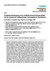
calculated, and the controller is directed to drive the robot to the next segment. When all segments are completed, the robot would be at the end point as desired. Figures 4 to 6, show the experimental trajectory tracking for the robot over the X, Y and Z Coordinates of the global coordinates system while Figures 7 to 9 show the orientation angles (Roll, Pitch and Yaw) tracking for both of the networks compared to each other verses the desired trajectory. The performance of the first network has improved when considering the Jacobian Matrix in the second configuration as Figures 4 to 9 show. 4.2 Testing Phase As the second configuration has shown better response than the first, it has been chosen to implement the testing data, new data that has never been introduced to the network before have been fed to the trained network in order to test its ability to make prediction and generalization to any set of data later overcoming problems resulting from applying the robot model. Testing data were meant to pass through singular configurations (fourth and fifth joints); these configurations have been determined by setting the determinant of the Jacobian matrix to zero. Table 3 shows the percentages of error for the testing data set for each joint. 4.2.1 Experimental Verification In order to verify the testing results, experiment has been performed to make sure that the output is the same or sufficiently close to the desired trajectory, and to show the combined effect of error, Figures 10 to 15 show the trajectory tracking of the X, Y, and Z coordinates with the Roll, Pitch and Yaw orientation angles respectively. The locus of which robot is passing through singular configurations are also shown. The error percentages in the experimental data are shown in table 4. Through these figures, it can be seen that a good prediction has been achieved .
5. Conclusions and Recommendations Inverse Kinematics problem is very important to be solved in close‐form for the robots using the Kinematics control approach, closed‐form analytical solutions can only be found for manipulators having simple geometric structures. A number of algorithmic techniques mainly based on inversion of the mapping established between the joint space and the task space of the manipulator’s
Jacobian matrix have been proposed for those structures that cannot be solved in closed form. In order to overcome the arising problems from applying the system kinematics model, which are mainly singularities and uncertainties in the arm configuration, Artificial Neural Network has been used trying to solve these problems. The proposed technique does not require any prior knowledge of the kinematics model of the system being controlled, the basic idea of this concept is the use of the ANN to learn the characteristics of the robot system rather than to specify explicit robot system model. Any modification in the physical set‐up of the robot such as the addition of a new tool would only require training for a new trajectory without the need for any major system software modification, which is a significant advantage of using neural network approach. In this research, two ANNs have been trained and compared. Comparison results shown that the performance of the network will be improved if considering the Jacobian Matrix in the solution. Euler representation has been used in this study to represent the orientation as a recommended by (Karilk and Aydin, 2000) as they have used the homogeneous transformation matrix to represent the orientation. For further research, we recommend a comparison study comparing the three types of orientation representation; in order to find the best orientation representation to be used. Backpropagation algorithm has been used as a learning algorithm with sigmoid transfer function as an activation function in all neurons, another recommendation we would like to recommend that a different learning algorithm, different activation function and/or different number of hidden neurons to be used in order to achieve, if possible, a better response in terms of precision and iteration. 6. References Antonelli, G., Chiaverini, S. and Fusco, G. A new on‐line algorithm for inverse kinematics of robot manipulators ensuring path‐tracking capability under joint limits. IEEE Transaction on Robotics and Automation 2003; 19(1): 162‐167. Bingual, Z., Ertunc, H.M. and Oysu, C., Comparison of Inverse Kinematics Solutions Using Neural Network for 6R Robot Manipulator with Offset. 2005 ICSC congress on Computational Intelligence. Denavit, J., and Hertenberg, R.S.A. Kinematics Notation for lower Pair Mechanism Based on Matrices. Applied mechanics 1955; 77: 215‐221.
14
Ali T. Hasan and H.M.A.A.Al‐Assadi: Performance Prediction Network for Serial Manipulators Inverse Kinematics solution Passing Through Singular Configurations
Driscoll, J.A. Comparison of neural network architectures for the modeling of robot inverse kinematics. Proceedings of the IEEE, south astcon .2000:44‐51. Duffy, J. Analysis of mechanism and robot manipulators, John Wiley, New York.USA 1980. Dulęba, I., Channel algorithm of transversal passing through singularities for non‐redundant robot manipulators. IEEE conference on Robotics and Automation, San Francisco, CA.USA2000: 1302‐1307. Dulęba,I., Sasiadek, J.Z., Redundant manipulators motion through singularities based on modified Jacobian method. Third International Workshop on Robot Motion and Control, November 9‐11,2002:331‐336. Fu, K.S., Gonzalez, R.C. and Lee, C.S.G. Robotics Control, Vision, and Intelligence. McGraw‐Hill book Co. Singapore, international edition. 1987. Funahashi, K.I. On the approximate realization of continuous mapping by neural networks. Neural Networks, 1998; 2(3): 183‐192. Hasan, A.T., Hamouda, A.M.S., Ismail, N., and Al‐Assadi, H.M.A.A. An adaptive‐learning algorithm to solve the inverse kinematics problem of a 6 D.O.F serial robot manipulator. Journal of Advances in Engineering Software 2006; 37: 432‐438. Hasan, A.T., Hamouda, A.M.S., Ismail, N., and Al‐Assadi, H.M.A.A. A new adaptive learning algorithm for robot manipulator control. Proceeding of the I Mech E, Part I: Journal of System and Control Engineering 2007; 221(4): 663‐672. Hornik, K. Approximation capabilities of multi‐layer feed forward networks.IEEE Trans.Neural Networks 1991;4(2):251‐257. Karilk, B., Aydin, S. An improved approach to the solution of inverse kinematics problems for robot manipulators. Engineering applications of artificial intelligence 2000; 13: 159‐164. Köker, R., Öz, C., Çakar.T. and Ekiz, H. A study of neural network based inverse kinematics solution for a three‐ joint robot. Robotics and Autonomous Systems 2004; 49: 227–234. Köker, R.,Reliability‐based approach to the inverse kinematics solution of robots using Elman’s networks. Engineering applications of artificial intelligence 2005; 18:685‐693. Kuroe, Y., Nakai, Y. Mori, T. A new Neural Network Learning on Inverse Kinematics of Robot Manipulators. International Conference on Neural Networks, IEEE world congress on computational Intelligence 1994; 5: 2819‐2824. Muszyński, R., Tchoń, K., Singularities of non‐redundant robot kinematics. Robotic Research 1997; 16(1): 60‐76. Nakamura Y., Advanced Robotics: Redundancy and Optimization, Addison Wesley, New York, USA.1991. Nakamura, Y. and Hanafusa, H. Inverse kinematic solutions with singularity robustness for robot manipulator control. Journal of Dynamic Systems Measurements Control 1986; 108: 163–171. 15
Tchoń K., Muszyński R., Singular Inverse Kinematic Problem for Robotic Manipulators: A Normal Form Approach”, IEEE Trans. on Robotics and Automation1998; 14 (1): 93‐104. Wampler, C. W. and Leifer, L. J. Applications of damped least‐squares methods to resolved‐rate and resolved‐ acceleration control of manipulators, Journal of Dynamic Systems Measurements Control 1988; 110: 31–38. Wampler, C. W. Manipulator inverse kinematic solutions based on vector formulations and damped least‐ squares methods. IEEE Transaction Syst., Man, Cybernetics 1986; 16: 93–101. Whitney. E. Resolved motion rate control of manipulators and human prostheses, IEEE Transaction Man–Mach. Systems 1969; 10:47–53.
International Journal of Advanced Robotic Systems, Vol. 7, No. 4 (2010)
1
2
3
4
5
6
5.9% 2.487% 2.703% 6.73% 6.803% 3.658% Table 1. Overall error percentages for the training data for the 6‐6 configuration. Joint 1 Joint 2 Joint 3 Joint 4 Joint 5 Joint 6 Angular Position 4.32% 1.408% 1.403% 4.237% 5.165% 1.623% Angular Velocity 2.627% 3.09% 2.33% 2.692% 2.803% 2.325% Table 2. Overall error percentages for the training data for the 7‐12 configuration. Joint 1 Joint 2 Joint 3 Joint 4 Joint 5 Joint 6 Angular Position 2.515% 0.29% 1.745% 10.065% 9.755% 1.78% Angular Velocity 4.2% 6.1% 3.22% 3.7% 6.5% 2.6% Table 3. Overall error percentages for the testing data (Simulation). Cartesian Trajectory Orientation Angles X Y Z Roll Pitch Yaw 3.72% 3.06% 1.042% 3.562% 6.2% 4.964% Table 4. Overall error percentages for the testing data (Experiment).
Fig. 1. Schematic diagram for a general 6DOF serial robot showing the wrist mechanism.
16
Ali T. Hasan and H.M.A.A.Al‐Assadi: Performance Prediction Network for Serial Manipulators Inverse Kinematics solution Passing Through Singular Configurations
Angular Position
2
1
X
Y
3
Z
Cartesian Position
4
5
6
Role Pitch Yaw
Orientation
Fig. 2. The topology of the 6‐6 Network configuration
Angular Position Cartesian Position Fig. 3. The topology of the 7‐12 Network configuration 17
Angular Velocity
Orientation
Linear Velocity
International Journal of Advanced Robotic Systems, Vol. 7, No. 4 (2010)
800 Desired 6- 6 Configurtion 600
7 - 12 Configuration
Distance ( mm )
400
200
0 0
50
100
150
200
250
300
350
400
-200
-400
-600 Time ( Sec. ) Fig. 4.Trajectory tracking of the X coordinate for both configurations compared.
1200
1000
Desired 6 - 6 Configuration
Distance ( mm )
800
7 - 12 Configuration
600
400
200
0 0
50
100
150
200
250
300
350
400
-200
-400 Time ( Sec. ) Fig. 5.Trajectory tracking of the Y coordinate for both configurations compared. 18
Ali T. Hasan and H.M.A.A.Al‐Assadi: Performance Prediction Network for Serial Manipulators Inverse Kinematics solution Passing Through Singular Configurations
2000 1800 1600
Distance ( mm )
1400 1200 1000 800
Desired 6 - 6 Configuration
600
7 - 12 Configuration
400 200 0 0
50
100
150
200
250
300
350
Time ( Sec. ) Fig. 6.Trajectory tracking of the Z coordinate for both configurations compared. 250 Desired
400
6 - 6 Configuration
200
7 - 12 Configuration
150
Angle ( Degree )
100 50 0 0
50
100
150
200
250
300
350
400
-50 -100 -150 -200 -250 Time ( Sec. )
Fig. 7. Orientation tracking of the Roll angle for both configurations compared. 19
International Journal of Advanced Robotic Systems, Vol. 7, No. 4 (2010)
80
Desired 6 - 6 Configuration
60
7 - 12 Configuration
40
Angle ( Degree )
20 0 0
50
100
150
200
250
300
350
400
-20 -40 -60 -80 -100 Time ( Sec. )
Fig. 8. Orientation tracking of the Pitch angle for both configurations compared.
250
Desired 6 - 6 Configuration 7 - 12 Configuration
200 150
Angle ( Degree )
100 50 0 0
50
100
150
200
250
300
350
400
-50 -100 -150 -200 -250 Time ( Sec. )
Fig. 9. Orientation tracking of the Yaw angle for both configurations compared. 20
Ali T. Hasan and H.M.A.A.Al‐Assadi: Performance Prediction Network for Serial Manipulators Inverse Kinematics solution Passing Through Singular Configurations
600
400 Desired Predicted Lucas of which robot is passing through Singular configuration in 2 Joints 2 DOF expected to be lost
Distance ( mm )
200
0 0
20
40
60
80
100
120
140
160
180
200
-200
-400
Lucas of which robot is passing through Singular configuration in 1 Joint 1 DOF expected to be lost
-600 Time ( Sec. )
Fig. 10. Experimental trajectory tracking of the X coordinate for the testing data.
1400
1200 Desired
Distance ( mm )
1000
Predicted
800 Lucas of which robot is passing through Singular configuration in 2 Joints 2 DOF expected to be lost
600
400 Lucas of which robot is passing through Singular configuration in 1 Joint 1 DOF expected to be lost
200
0 0
20
40
60
80
100
120
Time ( Sec. ) Fig. 11. Experimental trajectory tracking of the Y coordinate for the testing data. 21
140
160
180
200
International Journal of Advanced Robotic Systems, Vol. 7, No. 4 (2010)
Lucas of which robot is passing through Singular configuration in 2 Joints 2 DOF expected to be lost
2000 1800 Desired
1600
Predicted
Distance ( mm )
1400 1200 1000 800 600 400
Lucas of which robot is passing through Singular configuration in 1 Joint 1 DOF expected to be lost
200 0 0
20
40
60
80
100
120
140
160
180
200
Time ( Sec. )
Fig. 12. Experimental trajectory tracking of the Z coordinate for the testing data. Lucas of which robot is passing through Singular configuration in 2 Joints 2 DOF expected to be lost
200 180
Desired Predicted
160
Lucas of which robot is passing through Singular configuration in 1 Joint 1 DOF expected to be lost
Angle ( Degree )
140 120 100 80 60 40 20 0 0
25
50
75
100
125
Time ( Sec. )
150
175
200
Fig. 13. Experimental orientation tracking of the Roll angle for the testing data. 22
Ali T. Hasan and H.M.A.A.Al‐Assadi: Performance Prediction Network for Serial Manipulators Inverse Kinematics solution Passing Through Singular Configurations
80 60
Desired Predicted
40
Lucas of which robot is passing through Singular configuration in 2 Joints 2 DOF expected to be lost
Angle ( Degree )
20 0 0
20
40
60
80
100
120
140
160
180
200
-20 -40 -60
Lucas of which robot is passing through Singular configuration in 1 Joint 1 DOF expected to be lost
-80 -100 Time ( Sec. ) Fig. 14. Experimental orientation tracking of the Pitch angle for the testing data. 140 120
Lucas of which robot is passing through Singular configuration in 2 Joints 2 DOF expected to be lost
Desired Predicted
100 80
Angle ( Degree )
60 40 20 0 0
20
40
60
80
100
120
140
160
180
200
-20 -40 -60
Lucas of which robot is passing through Singular configuration in 1 Joint 1 DOF expected to be lost
-80 Time ( Sec. ) Fig. 15. Experimental orientation tracking of the Yaw angle for the testing data. 23