Performance Visualization and Exploration for ... - CiteSeerX

Performance Visualization and Exploration for Reconfigurable Computing Applications Seth Koehler and Alan D. George NSF Center for High-Performance Reconfigurable Computing (CHREC) ECE Department, University of Florida, Gainesville, FL, USA Abstract— Reconfigurable computing (RC) applications have the potential for significant performance while consuming little power. Although runtime performance analysis of RC applications has previously been shown to be important in achieving this potential, the optimization process is still arduous. We target two primary contributing factors: the incongruence between traditional CPU-based performance visualizations and RC performance data, and the need to manually predict the benefits of each potential optimization. To address these issues, we propose a methodology for interactive performance visualization targeted toward RC applications. Our methodology presents performance data hierarchically within the system and application contexts while simultaneously permitting a user to explore “what-if” scenarios to predict the effects of optimizations. We present a prototype of this visualization in our ReCAP (Reconfigurable Computing Application Performance) tool and demonstrate its utility via an application case study.

1. Introduction Reconfigurable computing (RC), which typically employs both CPUs and FPGAs, has been shown to provide substantial performance over using processors alone in a number of applications. Due to the complexity of these hybrid applications and systems, RC performance analysis (i.e., monitoring an RC application’s performance from within an RC device) has been shown to be important in achieving this potential [1], [2]. Unfortunately, even with current tools, the optimization process can still be difficult and time-consuming. Several factors complicate optimization. First, current performance visualizations are CPU-centric and do not reflect the heterogeneous, hierarchical parallelism common to RC applications, making it difficult to locate and understand performance bottlenecks. Second, once bottlenecks and potential optimizations are identified, the expected change in performance must be manually predicted for each optimization and weighed against other expected costs (e.g., implementation effort, power, resources used). Finally, due to the complexity of RC applications, the optimized application may still not meet desired performance, requiring additional optimization. In this paper, we seek to ameliorate these issues by proposing concepts and techniques for RC performance visualization and exploration that accelerate the optimization process; while we visualize and explore application performance within the

context of the system, our focus is on application (rather than system) performance. Section 2 provides background and related research for performance analysis, visualization, and performance prediction. In Section 3, we propose our methodology for RC performance visualization and provide details of a prototype visualization within our Reconfigurable Computing Application Performance (ReCAP) tool. Next, Section 4 overviews our methodology for performance exploration within this visualization, using runtime performance data to enable a user to perform “what-if” scenarios during the optimization process before implementing any changes. Finally, Section 5 provides a case study demonstrating the utility of our framework and tool, and Section 6 concludes.

2. Background and Related Research Performance analysis aides a user in quickly locating and remedying performance bottlenecks (see [3] for a good treatment of challenges and techniques). Performance analysis may be divided into stages including gaining access to application data (instrumentation), recording and storing data at runtime (measurement), optionally analyzing data for performance bottlenecks (automated analysis), visualizing performance data and analyses (presentation) that allow the user to carry on further analyses (manual analysis), and finally formulating and implementing optimizations to ameliorate bottlenecks (optimization). The process can be repeated if desired. Performance analysis can address metrics such as runtime performance, resource usage, or power consumption. These metrics may be interchangeable; for example, increasing application performance can allow fewer (or slower) devices to be used while still meeting performance requirements, potentially reducing the system cost or size. FPGAs, due to their reconfigurability, are even more flexible since application architecture and clock frequency can be changed, potentially trading performance improvements for lower power or fewer resources. Thus, improving runtime efficiency is often useful in achieving a balance among performance metrics. Since, RC applications are commonly programmed using high-level languages (HLLs) for CPUs (e.g., C/C++) and hardware description languages (HDLs) for FPGAs (e.g., VHDL, Verilog), it is beneficial to monitor performance from both portions of the application (as is done in our ReCAP framework and tool [1]). While HLLs can also be used to program an FPGA (and thus monitored as well [2]), we restrict

our focus to HDL-based applications. ReCAP monitors application performance via the HDL Instrumenter that instruments HDL code, the PPW+RC backend that instruments HLL code, and the PPW+RC frontend GUI that presents performance data post-mortem. PPW+RC components are extended from Parallel Performance Wizard (PPW), an open-source performance analysis tool for parallel programs [4]. ReCAP supports software written using C/C++, MPI, UPC, and SHMEM and hardware written using VHDL (Verilog support is in progress) using Xilinx ISE or Altera Quartus II tool-flows. Performance visualization seeks to rapidly convey application behavior to a user. While we found no previous work in visualization for RC applications beyond ReCAP, research in visualization for parallel applications suggests that visualizations should be concise, easy-to-use, informative, appropriate to the programming model, scalable, and interactive [5], [6]. Visualization can often benefit from a user’s high-level model of the application that is not present in (or not easily extracted from) source code, using this model to structure performance data in an intuitive, application-specific context (and potentially reducing instrumentation overhead as well) [7]–[9]. While we know of no work providing performance exploration for RC applications using runtime performance data, there is significant research in performance prediction during design space exploration (DSE). DSE employs analytical modeling or simulation to strategically explore alternative application designs or system architectures based on metrics such as performance, power, and resources. As generally no source code exists, the user supplies parameters or models of application or system behavior to predict performance. Balsamo et al. provide a good survey of performance-driven modeling techniques for software applications [10]. RC performance prediction using analytical models [11], [12] and simulation [9], [13], [14] has also been demonstrated. Finally, process algebras and calculi can be used to predict performance, from which we borrow some concepts for this paper [15].

3. RC Performance Visualization Unfortunately, traditional parallel-processor performance visualizations are not readily suited for RC applications. First, these visualizations typically assume devices are generalpurpose, interchangeable, and within a relatively shallow hierarchy (e.g., timeline visualization with one processor per row). In contrast, many components programmed on the FPGA are special-purpose (e.g., a component that scatters data to cores) and may be connected in arbitrarily deep hierarchies. If treated as a flat list of interchangeable devices, much of the structure and semantics of the application are lost. Second, even with heavily pipelined, superscalar processors executing instructions out-of-order, a single thread or process is still abstractly viewed as roughly sequential (since sequential ordering of application code is preserved), while a single FPGA component may perform an arbitrary amount of tasks in a given cycle (HDL code is inherently parallel). Finally, HDLs lack standardized, high-level communication and synchroniza-

tion functions (e.g., MPI_Send), complicating attempts to automatically classify and visualize such behavior. To address these issues, we follow a similar approach to [7], [8], having a user provide a high-level model of application behavior. However, to make our framework easy-to-use, we provide simple pragmas that allow a user to augment their source code with high-level information while not changing the application itself. Each pragma defines the current state of a hardware or software block (the finest-grained unit that operates in parallel with all other blocks, typically a software thread or process or a VHDL process block or Verilog always block); note that while the term “state” is used, no explicit state machine is needed in the application’s source code to employ our methodology. In software, pragmas are only used to classify FPGA API calls (since PPW, and therefore ReCAP, already monitors traditional parallel-program communication and synchronization). In hardware, pragmas are used to classify how time is spent in each clocked block. Figure 1 shows several examples of software and hardware pragmas. #pragma recap wrX send(top.in, data): words > 0 fpgaWrite(fpga, data, addr, words); ... #pragma recap waitDone wait_recv(top.out, done) while (fpgaReadReg(fpga, addr2) == 0);

(a) SW pragmas case current_state is when recvXCoord => --pragma recap getX recv($CPU,data) ... when waitAck => --pragma recap w1 wait_recv(top.out,ack):ack=‘0’ --pragma recap d1 recv(top.out,ack):ack=‘1’ ...

(b) HW pragmas Figure 1.

Example of user-defined pragmas

Each pragma-defined state is given a name and one or more classifications such as wait send, wait recv, send, recv, and busy (performing internal tasks), although other categories such as wait sync and overhead could be useful as well (the chosen categories are similar to those visualized in current performance tools [16] and used for performance modeling [15]). The “busy” category requires no arguments, while “wait” and “communication” categories require two arguments specifying dependencies and a “purpose” tag used to distinguish between similarly-typed messages from the same block. While a pragma automatically inherits all conditions that contain it, an optional condition field (after the colon) permits additional control over when a block is in a given state. Given this framework, we extended ReCAP to automatically monitor these pragma-defined states. While trace (timeline) information is ideal for viewing exact details of application behavior (and is supported by ReCAP on both CPUs and FPGAs), limitations on FPGA memory make it difficult to rely on such information. Instead, we build a Markov model of all CPU and FPGA blocks by recording time spent in each state and state transition, accepting a potential loss in fidelity. While this approach incurs O(n2 ) counters, where n is the number

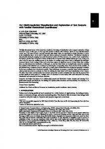
of states, it is common for many transitions to be impossible. Thus, we use a basic sparse-matrix representation for state transitions on both devices; due to the potentially high cost of implementing sparse matrices on FPGAs, we provide optional syntax in hardware pragmas to specify which transitions are possible, thus creating a static sparse matrix. A synthesis tool could potentially determine impossible transitions automatically, but this is difficult and may not be possible in all cases. To present performance in an intuitive, model-appropriate fashion, we visualize performance data within the system and application hierarchy. While HDL code is naturally hierarchical, we found the digraph generated from block dependencies better suited for understanding behavior than the actual structure of code (since HDL components or modules may simply pass data through or connect two sub-components together). For our visualization, we define the system, node, device, block, and state levels, allowing any of these levels to have one or more nested groups within it. A node is generally the smallest networked homogeneous unit of a system (which may contain multiple devices such as CPUs and FPGAs), while the block level refers to the definition of block given earlier (e.g., thread, VHDL process block), which are broken into states via user-supplied pragmas. Examples of application- or system-specific grouping include FPGAs on the same card and threads or cores performing similar tasks. By employing a hierarchical structure, scalability is improved and our visualization is appropriate to the hierarchical structure common in RC applications. As these levels are fairly generic, our visualization and exploration framework could also apply to other computing devices (e.g., GPUs, DSPs). In ReCAP, we prototyped this visualization (without grouping mentioned above) by generating a single file per logical CPU for use in Graphviz [17]; thus, multi-CPU/FPGA applications are supported, but the system-level view is not yet constructed. Graphviz can then generate scalable vector graphics (SVG) files, allowing a user to open the top-level SVG file and traverse the system and application hierarchy via hyperlinked nodes. Figure 2 shows actual tool-generated output for the device, node, and block levels, which have been cropped for brevity. The state level (not shown) is also visualized within our tool as an HTML table including the number of iterations, user pragma, source location, tool overhead, time spent in the state (including min, max, average, and total), and similar summaries of bytes transfered and communication bandwidth. Dependency information between blocks within the FPGA or between the FPGA and CPU are also visualized (e.g., the arrow connecting the two blocks within the device level in Figure 2). While visualization of CPU-CPU communication and synchronization is currently unimplemented in this view, statistical and timeline views of this behavior are available in PPW+RC’s frontend GUI. Figure 2 will be analyzed for performance problems in Section 5. The block level (for CPUs and FPGAs) shows each userdefined state’s name and type, along with the cumulative time spent in that state (numerically and visually via partially filled bars). In addition, transitions are labeled with a percentage

Node Level

Device Level (FPGA)

Block Level (CPU) Figure 2.

ReCAP visualizations for 2-core Collatz application

representing the frequency of a given transition in comparison to all outgoing transitions from the state. In CPU blocks, transitions are also labeled with the total time spent transitioning from one state to another (numerically and visually), as an arbitrary amount of work may occur between FPGA API calls. The CPU block level is shown at the bottom of Figure 2. At higher levels in the hierarchy, it is crucial to summarize data such that a user can quickly determine whether that item deserves further attention. From a performance analysis perspective, an application is performing ideally if all computational resources committed to the application are fully used; certainly better algorithms can have less utilization and still perform better, but performance analysis is concerned with maximizing a given solution, assuming all computation performed is necessary. Deviation from this ideal is considered

a (local) performance problem and potentially an application bottleneck (a critical performance problem degrading the entire application’s performance) and should be highlighted. Therefore, we display total time spent in each category when summarizing blocks within the device and node levels, and we display the maximum of each category’s totals (along with the minimum total busy time) for summarizing devices and nodes themselves. The maximum wait-time, communicationtime, and minimum busy-time show deviations from the ideal, while the maximum busy-time shows hot-spots that may benefit significantly from optimization (including algorithmic improvement). It may also be of use to provide standard deviation and automatic grouping or binning of blocks with other similarly performing blocks, depending on the application. Based on our visualization approach, it is often beneficial to define as few states as necessary to describe high-level application behavior, inserting additional pragmas in key areas if more detail is needed. In addition, while hierarchical structuring has many advantages, it may also be desirable to query or aggregate performance data. For example, a query such as SELECT * FROM FPGA[*] WHERE TIME(SEND) > 0.1*TOTAL_TIME() could be used to find all FPGA states sending data more than 10% of the time. Due to significant implementation cost, this feature is not currently implemented.

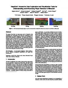
law suggests an ideal speedup of 22.9% (1/(1 − 3s/10.75s + 3s/10.75s )) is possible. However, in reality, the performance 3 of other blocks could inhibit us from achieving this potential. Assuming the average case, the above optimization will reduce each of the four iterations of busy2 by 0.5s, leaving gaps in Block B’s timeline (Figure 4b). Unfortunately, the first three gaps precede a wait state; since Block B was already waiting on Block A, Block B will have to wait that much longer. However, the final gap is followed by communication with Block A, where Block A is waiting for this communication. Thus, Block A could now wait less time, allowing the final send/recv pair to complete 0.5s earlier (Figure 4c) and providing a final speedup of 4.9%, much less than the ideal 22.9% (this ideal could be realized with a similar change to busy1 instead). 1

busy1

1 5s

wait2

3

4

send1

recv2

4s 1

wait1

0.75s

4s

busy2

2

3

3s 1

send2

1s 1

1s 1

Block A (10.75s) Figure 3.

7

4

1

recv1

2.75s 4

Block B (10.75s)

Example application for exploration.

4. RC Performance Exploration Once performance is visualized, the user must formulate potential optimizations and weigh expected performance gains against expected costs of optimization (e.g., effort, power, resources). Unfortunately, predicting performance can be difficult in complex RC applications, potentially leading to wasted implementation effort. As mentioned in Section 2, DSE is invaluable for providing early performance estimates. However, these estimates may be inaccurate due to assumptions concerning the system and application; thus, we employ actual performance data gathered for our visualization to support performance exploration in the optimization stage. Our proposed exploration methodology compliments existing methods in DSE and performance prediction. Since our goal is to maximize performance of an existing system and design, we take advantage of detailed performance data, targeting finergrained changes and more accurate exploration rather than broad changes common in traditional DSE. Ideally, our data and methodology could be integrated with existing DSE tools (e.g., augmenting application and system models with real performance data), enabling more accurate prediction and providing an end-to-end environment in which to study application performance, from conceptual design through optimization. We now motivate our approach. Figure 3 shows mockup performance data for an application consisting of two blocks. Each state contains the cumulative time (CT) spent in that state (over all iterations) as well as the number of incoming and outgoing transitions, from which a potential timeline can be constructed (Figure 4a). Supposing an optimization could reduce the CT of the busy2 state from 3s to 1s, Amdahl’s

Wait

Comm

Busy

A B

10.75s (a) Initial timeline

A B gaps (b) After local modification

A B increase in wait

10.25s

decrease in wait (finish 0.5s earlier)

(c) Final result Figure 4.

Potential timelines when optimizing an example application.

While the previous example focused on changing a state’s CT (along with the corresponding adjustments to other states), other changes can be modeled as well. For example, changing FPGA clock frequency can be modeled as scaling the total time of each FPGA state (except those communicating or waiting on external resources such as SRAMs or CPU). Changing a block’s replication factor by F (e.g., doubling

CPUs or FPGA cores) can be modeled as scaling all busy and communication state times by a factor of 1/F (assuming perfect load balancing). Our framework does not constrain the magnitude of such changes, allowing users to investigate performance if a larger or faster device were employed; however, potential changes in resource usage and achievable frequency should be considered when targeting specific devices. Ideally, a tool could automatically map these higher-level changes into corresponding state-level changes rather than requiring the user to manually perform this mapping. This approach makes several assumptions. Since a generated timeline represents the average case, it could differ significantly from actual runtime behavior (especially with shared effects such as contention). However, a number of RC applications exhibit very regular behavior, and thus our approach is reasonable given the significant memory reduction afforded by using summary statistics (even trace data can be insufficient to predict performance as a single execution may not include all execution paths). Also, although a user’s change to the CT of one or more states could affect the CT of a busy or communication state, we assume only the CT of wait states is adjusted, as this case is far more common and easier to model. Finally, although matching communication states between blocks can wait on each other (e.g., in one iteration Block A waits on Block B while in the next Block B waits on Block A), we assume that communication can be shifted such that only one block is waiting on another; while not always possible, this represents an ideal case if such a synchronization problem is remedied. We show in Section 5 that our methodology can still be fairly accurate, even with non-uniform behavior. Unfortunately, generating timelines consistent across all blocks can be difficult, as matching send/recv pairs must be aligned globally (e.g., in Figure 4a, Block B’s first wait state was elongated in order to line up communication states). Thus, for simplicity and efficiency, we forego timeline generation, instead employing a heuristic methodology that calculates the CST, or cumulative time a state is shifted in the timeline (e.g., the final -0.5s shift in Figure 4c), as well as the CT for each state; pseudocode for our approach is provided in Figures 5 and 6. Note that while CST/CT calculation may yield different results from a timeline approach (as the latter ensures matching transfers occur together rather than just ensuring that dependencies, on average, are met), this does not imply the timeline approach is more accurate; both are effectively assuming a schedule that may differ from actual execution. We now re-predict performance for our example application via the CST/CT methodology. As shown in Figure 7a, the user changes the CT of busy2 from 3s to 1s (checkered). The propBlk function (Figure 5) is then called with the busy2 state and -2s CST. This function is responsible for propagating a change in expected CST throughout a block, adding any dependencies to a queue for later processing. The CST is split among all potential next states based on the frequency of transitions to each. If a state has been visited before, the handleCycle function (definition not shown) finds all states outside the cycle that have a transition to them from

void propBlk(State s, double CST) { if (CST == 0) return; s.CST += CST; // add dependencies to queue foreach (dep in s.dependencies) depQueue.add(dep); // compute next state changes double total = sum(s.outTrans); foreach (n in s.nextStates) { double frac = s.outTrans(n) / total; if (n.visited) handleCycle(n, s, frac * s.CST); else propBlk(n, frac * s.CST); }} Figure 5.

sw.CST

Block-propagation methodology

sw

s s.CST Source

dw

dw.CST

d

d.CST Destination

void handleDep(State s, State sw, State d, State dw) { double CST, CT; // modify wait times CST = max(-dw.CT, s.CST – d.CST); CT = min(CST, max(CST – sw.CT, 0)); dw.CT += CT; sw.CT += CT – (s.CST – d.CST); // propagate and back-propagate propBlk(dw, CT); propBlk(sw, CT – (s.CST – d.CST)); } Figure 6.

Dependency-handling methodology

within the cycle (exit states) and determines the correct split of CST between these states (determined either by iteration or geometric series if the number of iterations is sufficiently large). In our example application, the call to propBlk adds dependencies for recv2 and send2 to the queue and results in the final CST values shown (black ellipses) in Figure 7a. At this point, each dependency is incrementally applied by calling handleDep with the four relevant states in the dependency: the source s, its corresponding wait state sw, the destination d, and its corresponding wait state dw (Figure 6). If there is no corresponding wait state for either s or d, an implicit one with zero CT is added. The handleDep function attempts to shift communication as early as possible, resolving any conflict detected by increasing wait time at the source. Figure 7b shows the result of triggering the recv2 dependency, which resolves a conflict where Block B could progress faster but Block A cannot, thus increasing the wait time in wait2 to 4.25s. Figure 7c then shows the final outcome after triggering the send2 dependency, which allows the recv1 state in Block A to shift 0.5s earlier (by reducing the CT of wait1 to 0.25s), yielding a final reduction of 0.5s out of 10.75s (4.9% speedup) for the application, as predicted earlier. Note that our methodology not only predicts overall performance, but also the CT for each state, thus aiding a user in locating and

4

send1

4s 1

wait1

0.75s 1

recv1

1

0s 5s

1s

wait2

3

-1.5s 2.75s

4

0s

recv2

4s 4

0s 2

busy2

1s 1

0s

send2

1

1s

7

-1.5s 3

-2s -2s

1

Block A (10.75s)

Block B (8.75s)

(a) Result of initial update to Block B 1

busy1 4

send1

4s 1

wait1

0.75s 1

recv1

1

0s 5s

1s

wait2

3

0s 4.25s

4

0s

recv2

4s 4

0s 2

busy2

1s 1

0s

send2

1

1s

7

0s 3

-0.5s -0.5s

1

Block A (10.75s)

Block B (10.25s)

(b) Result of recv2 dependency handling 1

busy1 4

send1

4s 1

wait1

0.25s 1

recv1

1

0s 5s

1s 1

Block A (10.25s)

wait2

3

0s 4.25s

4

0s

recv2

-0.5s 2

-0.5s

4s 4

busy2

1s 1

send2

1s

7

0s 3

-0.5s -0.5s

1

Block B (10.25s)

(c) Result of send2 dependency handling Figure 7.

Performance exploration using CST/CT updates

potentially remedying bottlenecks in an optimized version of the application before the optimization has been implemented. While our intent is to allow users to modify a state’s CT, block replication, or frequency within our visualization, performance exploration is not currently implemented in ReCAP. Thus, we manually employ our exploration framework to demonstrate its utility.

5. Results To validate the utility of our framework, we investigate the performance of a Collatz application, which tests the lengths of sequences generated under repetitive iteration of a simple function on the natural numbers (see [18] for details). While this application is not readily used for practical purposes, it contains patterns that closely resemble cryptanalysis (i.e., a large number space is pre-filtered by a CPU, the FPGA performs a large parallel search, and finally the CPU collects and performs post-processing on returned numbers) [19], [20]. In addition, both the CPU and FPGA are involved in computation, with FPGA cores requiring an unknown number of cycles to complete, thus providing a case study that would be difficult to predict performance for via other methods. The application was executed on a Pentium-4 3.2GHz 64bit Xeon processor containing a Nallatech H101-X PCI-X

card with a Virtex-4 LX100. We used GCC 4.4.2 with “O3” optimization and Xilinx ISE 11.3 with default settings to compile the application software and hardware, respectively; the same application served as a C baseline (with FPGA tasks performed on the CPU instead). All execution times were computed from the average of three executions, with the FPGA operating at 100MHz. Each execution consisted of running sequence-length tests on the first 154 billion numbers. Figure 2 shows visualizations generated by ReCAP for an initial 2-core version of the Collatz application. From the visualizations, we quickly noticed the CPU is waiting a significant amount of time for the FPGA to complete its work (100.8s, as shown in the CPU-block-level visualization), representing poor hardware/software partitioning that could be remedied easily by increasing the number of cores in the FPGA. Assuming the wait-time problem can be removed, the inStatus1 state is taking up a significant portion of the remaining time (13.5%). Decreasing the transmission frequency (and correspondingly increasing buffer size) could reduce this overhead. In support of this decision, clicking on the send1 state indicates an average bandwidth of 42.5MB/s and message size of 0.75KB (not shown); platform benchmarks indicated that increasing message size could improve bandwidth significantly. We now predict the effects of scaling the number of FPGA cores in our application from 2 to 56 via our performance exploration methodology (64 cores could not be validated due to FPGA resource limitations). Figure 8 shows the ideal prediction given by Amdahl’s law (triangles), our methodology’s prediction (squares and dotted line), actual application performance (asterisk), and performance achieved from an optimized version of the application discussed below (circles). Since FPGA computation represents the majority of the application time, Amdahl’s law predicts near-linear speedup, with a 56-core version achieving a total 54.2x speedup over the software baseline. However, our performance exploration predicts that performance will scale in a roughly linear fashion until leveling off around 12 cores, with the 56-core version achieving a total 12.1x speedup over the software baseline. 60

Speedup (vs. CPU)

1

busy1

50 40

Amdahl

361% error

3.8x speedup

30 20 10

ReCAP Actual Optimized

0 2

4

8

16

32

Number of Cores

Figure 8.

56

3.3% error

Performance exploration for Collatz application.

Our actual 56-core version achieved a total 11.7x speedup over the software baseline, resulting in a maximum error in predicted performance of only 3.3% for our performance exploration methodology (using Amdahl’s law yields 361%

error), thus demonstrating our framework’s utility, even in the presence of non-uniform behavior. As examining the predicted state CTs indicated the FPGA would be mostly idle if 56-cores were employed, we developed an auto-tuning step to perform coarse-grained load-balancing between the CPU and FPGA and reduced transmission frequency (as mentioned earlier), yielding a 3.8x speedup over the original 56-core design (44.7x speedup over the software baseline), as shown in Figure 8. Due to the number of application resources used (85% LUTs, 32% regs, and 57% block RAMs (BRAMs)), we chose to instrument only 2 of the 56 hardware cores (all other software and hardware were instrumented normally). We observed a change of +1.7% (or less) in software runtime, -2% LUTs, +4% regs, +35% BRAMs, and no change in maximum frequency. The unexpected changes to LUTs and BRAMs were due to instrumentation interfering with a RAM-packing synthesis optimization that decreases BRAMs at the expense of LUTs. Unfortuntaely, ReCAP replicates components in loops to ease instrumentation, preventing ISE from detecting this optimization for this application; better handling of loops in ReCAP would avoid this issue. Disabling this optimization yields a more informative baseline of 77% LUTs, 32% regs, and 92% BRAMs for the original application, yielding an actual overhead of +6% LUTs, +4% regs, and +0% BRAMs.

6. Conclusions In conclusion, we provided a methodology for both performance visualization and performance exploration of RC applications, implementing a prototype visualization within our ReCAP tool. We then demonstrated the utility of our framework and tool by predicting application performance before actually implementing changes, yielding only 3.3% error when validated. Based on these results, a scalability problem and inefficient communication were quickly located and remedied, yielding a 3.8x speedup of our original 56-core design (increasing application speedup from 11.7 to 44.7 when compared to the software baseline). Future work includes implementing the exploration framework and potentially integrating both into DSE tools, allowing users to follow application performance through the entire design process. In addition, handling more complex scenarios, including modeling buffers and memories as well as including trace data, could be of use.

Acknowledgments This work was supported in part by the I/UCRC Program of the National Science Foundation under Grant No. EEC0642422. The authors gratefully acknowledge vendor equipment and/or tools provided by Aldec, Altera, Nallatech, and Xilinx.

References [1] S. Koehler, J. Curreri, and A. D. George, “Performance analysis challenges and framework for high-performance reconfigurable computing,” Parallel Computing, vol. 34, no. 4-5, pp. 217–230, 2008.

[2] J. Curreri, S. Koehler, A. D. George, B. Holland, and R. Garcia, “Performance analysis framework for high-level language applications in reconfigurable computing,” ACM Trans. on Reconfigurable Technology and Systems, vol. 3, no. 1, pp. 1–23, 2010. [3] S. S. Shende and A. D. Malony, “The TAU parallel performance system,” Int. Jour. of High Performance Computing Applications (HPCA), vol. 20, no. 2, pp. 287–311, May 2006. [4] H.-H. Su, M. Billingsley, and A. D. George, “Parallel performance wizard: A performance analysis tool for partitioned global-address-space programming,” in IEEE Int. Symposium on Parallel and Distributed Processing (IPDPS’08), April 2008, pp. 1–8. [5] B. P. Miller, “What to draw? When to draw?: an essay on parallel program visualization,” Jour. of Parallel and Distributed Computing, vol. 18, no. 2, pp. 265–269, 1993. [6] M. T. Heath, A. D. Malony, and D. T. Rover, “Parallel performance visualization: From practice to theory,” IEEE Parallel and Distributed Technology, vol. 3, no. 4, pp. 44–60, 1995. [7] J. Garc´ıa, J. Entrialgo, and D. Garcia, “An instrumentation and visualization technique for performance analysis of high-performance industrial embedded applications,” in Proc. of the 16th IEEE Instrumentation and Measurement Technology Conf. (IMTC’99), vol. 2, 1999, pp. 958–963. [8] M. Sefika, A. Sane, and R. H. Campbell, “Architecture-oriented visualization,” in Proc. of the 11th ACM SIGPLAN Conf. on Object-oriented Programming, Systems, Languages, and Applications (OOPSLA ’96). New York, NY, USA: ACM, 1996, pp. 389–405. [9] K. Bondalapati and V. K. Prasanna, “DRIVE: An interpretive simulation and visualization environment for dynamically reconfigurable systems,” in Proc. of the 9th Int. Workshop on Field-Programmable Logic and Applications (FPL’99). Springer Berlin / Heidelberg, 1999, pp. 31–40. [10] S. Balsamo, A. Di Marco, P. Inverardi, and M. Simeoni, “Model-based performance prediction in software development: a survey,” IEEE Trans. on Software Engineering, vol. 30, no. 5, pp. 295–310, May 2004. [11] M. C. Smith and G. D. Peterson, “Parallel application performance on shared high performance reconfigurable computing resources,” Performance Evaluation, vol. 60, no. 1-4, pp. 107–125, 2005. [12] B. Holland, K. Nagarajan, C. Conger, A. Jacobs, and A. D. George, “RAT: a methodology for predicting performance in application design migration to FPGAs,” in Proc. of the 1st Int. Workshop on Highperformance Reconfigurable Computing Technology and Applications (HPRCTA’07). New York, NY, USA: ACM, 2007, pp. 1–10. [13] D. Densmore, A. Donlin, and A. Sangiovanni-Vincentelli, “FPGA architecture characterization for system level performance analysis,” in Proc. of the Conf. on Design, Automation and Test in Europe (DATE’06). 3001 Leuven, Belgium, Belgium: European Design and Automation Association, 2006, pp. 734–739. [14] C. Reardon, E. Grobelny, A. D. George, and G. Wang, “A simulation framework for rapid analysis of reconfigurable computing systems,” ACM Trans. on Reconfigurable Technology and Systems (TRETS), to appear. [15] A. Clark and S. Gilmore, “State-aware performance analysis with extended stochastic probes,” in Proc. of the 5th European Performance Engineering Workshop on Computer Performance Engineering (EPEW’08). Berlin, Heidelberg: Springer-Verlag, 2008, pp. 125–140. [16] Z. Szebenyi, B. J. Wylie, and F. Wolf, “Scalasca parallel performance analyses of PEPC,” in Proc. of the 1st Workshop on Productivity and Performance (PROPER) in conjunction with Euro-Par 2008, ser. Lecture Notes in Computer Science, vol. 5415. Springer, 2009, pp. 305–314. [17] J. Ellson, E. Gansner, L. Koutsofios, S. C. North, and G. Woodhull, Lecture Notes in Computer Science: Graph Drawing. Springer Berlin / Heidelberg, 2002, ch. Graphviz - Open Source Graph Drawing Tools, pp. 594–597. [18] J. C. Lagarias, “The 3x + 1 problem and its generalizations,” The American Mathematical Monthly, vol. 92, no. 1, pp. 3–23, Jan. 1985. [Online]. Available: http://www.jstor.org/stable/2322189 [19] J.-J. Quisquater, F.-X. Standaert, G. Rouvroy, J.-P. David, and J.-D. Legat, “A cryptanalytic time-memory tradeoff: First FPGA implementation,” in Field-Programmable Logic and Applications: Reconfigurable Computing Is Going Mainstream. London, UK: Springer-Verlag, 2002, pp. 780–789. [20] T. Pornin and J. Stern, “Software-hardware trade-offs: Application to A5/1 cryptanalysis,” in Proc. of the 2nd Int. Workshop on Cryptographic Hardware and Embedded Systems (CHES’00). London, UK: SpringerVerlag, 2000, pp. 318–327.