Grey-Level Dependence Method (SGLDM); it shows the distribution of the intensities of pairs of ... existing techniques while adapting to the specifics of the ultrasonic image obtained in NDT. ... replacing the manual thresholding with an automatic ... a threshold, the only common aspect used in previous .... main inertia axes.
Pattern Recognition, Vol. 29, No. 2, pp. 281 ~96, 1996 Elsevier Science Ltd Copyright © 1996 Pattern Recognition Society Printed in Great Britain. All rights reserved 0031 3203/96 $15.00+.00
Pergamon
0031-3203(95)00082-8
BSCAN IMAGE SEGMENTATION BY T H R E S H O L D I N G USING COOCCURRENCE MATRIX ANALYSIS* G. C O R N E L O U P , t J. M O Y S A N t and I. E. M A G N I N ++ "~Laboratoire de Contr61e Non Destructif, MECASURF-LCND (EA 1429), G.M.P., I.U.T. Aix, 13625 Aix en Provence, France :~Laboratoire de Traitement du Signal et UltraSons, URA CNRS 1216, INSA Lyon, 69621 Villeurbanne, France (Received 29 July 1994; in revised form 12 May 1995; received for publication 2 June 1995) Abstract--In this paper we present innovative research for the processing of an ultrasonic image obtained in non-destructive testing (NDT). We also present an algorithm for automatic thresholding segmentation. The image analysis is based on the calculation of cooccurrence matrices. The method we used is the Spatial Grey-Level Dependence Method (SGLDM); it shows the distribution of the intensities of pairs of pixels separated by a vector d. We show that it is necessary to build optimized matrices in order to improve the existing techniques while adapting to the specifics of the ultrasonic image obtained in NDT. We solve for the vector d through an automatic analysis of the matrix behaviour for several vectors based on the characterization curves. The developed method allows us to present an efficient thresholding algorithm that is tested on real images. Image processing
Segmentation
Threshold
1. INTRODUCTION The possibilities of non-destructive testing by ultrasonic images have been improving steadily since the appearance of computing systems that are able to process the recorded signals rapidly and create images specific to this type of testing. "'2~ The type of images we present in this paper do not have much of a history of research in terms of image processing analysis (cf. Fig. 7). However, it can compare, in principle, with those obtained in the medical field with the echography technique. There is, therefore, on these images no processing likely to be used as a reference or standard except for results obtained by a qualified expert. This type of testing is first aimed at detecting one or several possible defects on the image. It is very important to obtain the size of defects in N D T and to know what type of defect it is. F o r example, the size of a crack can be included in a fracture mechanics calculation to be able to forecast the lifetime of the cracked object. F r o m the standard conception of testing by ultrasound, we searched for an event with an amplitude above the ground noise. The initial idea consisted of replacing the manual thresholding with an automatic one in order to be in a position to process the vast quantities of data. (3~ The physical constitution of the ultrasonic signals leads to perfectly unimodal histo-
* This research was carried out in collaboration with the LCUS Laboratory (Laboratoire de Contr61e par UltraSons, Saclay, France) of the CEA (French Atomic Energy Commission). 281
Cooccurrence matrix
Ultrasounds
grams that are not likely to provide suitable results if exploited with the methods used for simple histograms. (4) Indeed, the obtained defect signals are similar to a sinusoid multiplied by a Hamming's function, so that the distribution of amplitude linked to the defects does not distinguish from that of the ultrasonic signal sent back by a defectless zone. Consequently, we tried to increase the quality of the obtained information by means of the application of a two-dimensional (2-D) processing that defines a threshold and takes into account the a priori knowledge from the spatial aspects of the image. As a matter of fact, as quoted by Haralick, (5/it is certain that a priori introduction of information into a segmentation method is the key element to improving the results. We took an interest in the 2-D histogram or cooccurrcnce matrix. This tool (6'7) was selected for the present study as several general considerations were favourable: first, the images assume a textured aspect due to the frequency of the transducer in use; secondly, the echos of the defects have angular orientation in the image; and finally, previous studies had good results in threshold definitions from the cooccurrence matrix ~s 11) (cf. Fig. 7). In order to be able to respond fully to the study of the spatial and angular relations between the background of the image and the defects, we opted for the more general definition of the cooccurrence matrix, using the spatial grey-level dependence method ( S G L D M ) J 12'13) With this approach the distribution of the pairs of pixels in the image separated by a vector d defined by its modulus and orientation is under consideration. Other studies that are based on texture
G. CORNELOUP et al.
282
analysis exploited the cooccurrence matrix for the segmentation of images.(15-17) The definition of a threshold, the only common aspect used in previous studies, is decisive in this type of study. The thresholding from the cooccurrence matrix was developed by Weska. (s) The technique consisted of evaluating the distribution of the cooccurrence matrix coefficients through a function named Busyness. Other authors then presented various functions of matrix analysis to determine one ~9'1°) or several thresholds/~) The study of the use of large-dimension d vectors made possible from an extension of the definition of the SGLDM method showed that we could construct cooccurrence matrices which are very different from the common matrices which exploit the relation between close pixels. In this study we shall call the common matrices A-type matrices, and B-type matrices those that exploit large spatial relations. We shall show what the new matrices are, as well as their interest. To meet the objective of defect detection in the BSCAN image with this new type of matrix we shall present a new development of the threshold definition method with the cooccurrence matrix analysis. Section 2 shows how the SGLDM approach allows the extension of the representation possibilities of information through the cooccurrence matrix. This means mastering an important parameter: the vector d. We specifically developed a new approach of the cooccurrence matrix analysis based on a search for the background/boundary information. In parallel we considered a new approach for the threshold calculation through the analysis of the dispersion of the matrix coefficients. Section 3 shows that it is possible to automate the method in order to select automatically a vector d. Section 4 provides the general algorithm. The results on images of weld testing and the discussion is presented in Section 5. 2. D E F I N I T I O N OF THE MATRIX A N D T H R E S H O L D I N G CURVES
2.1. Definition of the matrix The construction of the cooccurrence matrix with a vector d allows us to exploit all the possibilities of spatial relations between the objects of an image without restricting them to the neighboring pixels17'11) or to a set of fixed directions.~11,12,16) The BSCAN image is a two-dimensional function f defined on a finite and discrete domain D of M by N dimensions. The function f represents the pixel's intensity and has its values in a discrete set E of K elements {0, 1..... K -- 1}, usually K equals 256. The cooccurrence matrix is a function of two variables i and j, the intensities of two pixels, each in E; it takes its elements in N (set of natural integers). The parameters are the image f and the vector d, whose Cartesian coordinates are dx and dy and whose polar coordinates are r and 0. The cardinal number of the set A~j
gives the number of occurrences on the image f of pairs of pixels separated by vector d; the latter pairs have i a n d j intensities respectively, i.e.
c:ExE~ (i,j)~--~c(i,j,f,d_) = IAijI
(1)
If we call td, which is the translation whose vector takes the value of vector d, and if we use the symbol of intersection (n) for two sets, then the set Aij can be defined as follows:
Aij = { ((x, y), (x', y'))l(x, y)D c~ t _ n(D), (x', y')D n t d(D ) and (x', y ' ) = td(x, y) and f ( x , y) = i and f(x', y') =j}.
(2)
This definition implies that the direction of vector d was taken into account and that the coefficient c(i,j,f,d) and c(j,i,f,d) may be different. The coefficients were standardized by the division of each coefficient by the sum A of all the coefficients. The normalized coefficient p(i,j,f,d) thus corresponds to a joint conditional probability of the event (i,j) occuring. The value of A depends on vector d:
A = JDc~td(D)l + IDc~t d(D)l = 2(M --tdxl)(N -Idyp). (3) We built a symmetrical matrix. Thus, both the distance and the angle of vector d determine the values of the matrix independently of the direction. So, the number of the matrix coefficients used for matrix analysis will be reduced by half. The symmetrical matrix consists of a two-step operation:
Cij=p(i,j,f,d)+p(j,i,f,d),
for every / in [ 0 , K - 1] andj < i (4a)
C~i = Cir.
(4b)
An asymmetrical definition allows to obtain more detailed information in which the direction of the vector is prominent. Its analysis, which is more complex, must be reserved for issues for which it is necessary, e.g. analysing the reflected shadows on photographs or examining the amplitude asymmetry of some ultrasonic signals which form the images obtained in NDT. 2.2. Coefficients of a spatial dependence matrix Prior to examining how the cooccurrence matrix is used to define a threshold, let us consider in what way the information of the image is present in the matrix. With the SGLDM, there are several possibilities to exploit the cooccurrence matrix. We defined the minimum and the maximum sizes of the objects in the image as dirm3nin(0) and dim~nax(0). These dimensions depend on the analysis angle of the image corresponding to the analysis angle of vector d. Figure 1 shows simplified construction of matrices obtained for the two types of images, each containing two objects. We considered a classical image named video type (a) (e.g. radiography) on which one object has a mean intensity that is different from the intensity
BSCAN image segmentation
283
~-=$ "=
b a
d
(ko,y)
,d3 9
a) classical image
b a
"~
-?V
b
""
i(x0,y)
2
d) image HF
i
!
L
d=d 1]
,,+,,i ,',°
ja
p.+a[~_ j, _
i ~7
(1) d=d 3
a I
e) matrix A
b) matrix A
~ ~ ..= "=+ ,.+ b
a
i (1),,\
-
bE aD
q
i-~.12/
1) 1
d=d
7
(1) d = d 4
(1) d=d 3
(2) d=d 5
I I
•
1
j
~
,
/
J
f) matrix B
c) matrix B •
background
[ ] objects
[ ] transitions
[ ] interactions
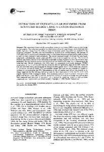
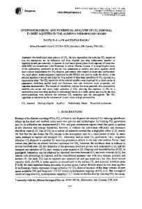
Fig. 1. Matrix description from two types of images. (a) Classical image showing column at position Xo, (b) A-type matrix from image a, (c) B-type matrix from image a, (d) HF image showing column at position x0, (e) A-type matrix from image d and (f) B-type matrix from image d.
of the noise [Fig. l(a)]. The second type of image is one where the amplitudes of one object are either side of the mean value /~ [Fig. l(d)]. This type of image corresponds to an unfiltered ultrasonic image known as the HF-type image, on which the object of the image corresponds to a distribution of the sinusoidal type multiplied by a Hamming's window in both directions of the main inertia axes. If the ultrasonic image is filtered and rectified, an ultrasonic image similar to a classical one is obtained. We shall henceforth consider these two types of images in the following part of this paper. We have represented the four types of pairs of pixels that are built with four symbols:
(1) background pair: both pixels belong to the background (black square); (2) object pair: both pixels belong to the same object (white square); (3) inter-action pair: the two pixels belong to two objects (hatched square); (4) boundary pair: one pixel belongs to the background of the image and the other belongs to an object (square with dot). If we use a vector d with a low modulus [d = dl see on Fig. l(a) and l(d)], less than d i ~ i n ( 0 ) , we then build a matrix in which the coefficients lie along the
284
G. CORNELOUP et al.
diagonal considering that the transition between the background of the image and the top of the object is slow. Let us call this type of matrix an A-type matrix [cf. Fig. l(b) and l(e)]. It is the very type of matrix which is most commonly exploited in texture analysis, as the relations with the neighboring pixels are under consideration. The search for thresholds, and hence for objects in this type of matrix, is close to an analysis of the modes of the simple histogram, the matrix coefficients' peaks along the diagonal being representative of the various objects. (17/ If we use a vector whose modulus is greater than dim_max(0) [ d = d2 see Fig. l(a) and l(d)], we will obtain a representation of the information on the transitions between background and objects or even between objects. This representation will be named hereafter as type B matrices [cf. Fig. l(c) and l(f)]. In the case that concerns us we can assume that a single threshold will allow the isolation of the objects in the image, this very background/object information is
[]b
a
>i
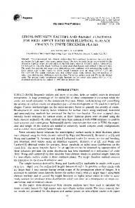
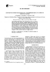
what we will try to obtain in order to bring out the b o u n d a r y between background and objects. It is possible that objects are not directly represented in a matrix. Thus, in matrices (c) and (f) the pairs of objects disappear and interaction pairs may appear according to the value of vector d. Let us now examine how these different distributions of the coefficients, which are different presentations of the information, can be exploited to define a threshold. 2.3. Division o f matrix The position of a threshold value t in the cooccurrence matrix divides the matrix into four blocks (al [Fig. 2(a)]. To present the problem we shall first consider the case of Fig. 2(a), where the image is made of a uniform background and objects of different intensities [Fig. l(a)]. The matrix coefficients represent three categories of coefficients. A threshold t may separate these categories on condition that their repre-
~t-a~
[
i
It rq(1)
i
[~ ID(1)
d=d I
~+b " -- 1)--D- "~ ~+a 1 ;
!
a
\
I
EL
\
(1) d = d 2
\
/i
1\\ b
[ I
1
c) matrix A
a)matrixA ~:~b
I
",\
d=d 3
a~
(~) d=d 4 (1) d=d 3
\,\ \\
(2) d=d 5
\
J b) matrix B
•
background
[ ] objects
d) matrix B
[ ] transitions
[ ] interactions
Fig. 2. Division of the matrix and threshold positions. Same vectors d as for Fig. 1: A-type matrix from image l(a), (b) B-type matrix from image l(a), (c) A-type matrix from image l(d) and (d) B-type matrix from image l(d).
BSCAN image segmentation sentations in the matrix be possibly connected to the successive splitting of the blocks B~= ~,4[t]. From the classical definition of the matrix (8-~ ~) the basic idea for the exploitation of these relations concerns video-type images with a vector d that is short compared with the dimensions of the objects. Figure 2(a) displays a division with a pertinent threshold of the matrix. In the block B1 [t] the included coefficients belong to the background of the image, on the contrary in the block B4[t] the coefficients correspond to the objects of the image, finally the blocks B2[t] and B3 [t], made identical by the construction of a symmetric matrix, contain the coefficients libked to the transitions between background and objects. For this type of analysis, the coefficients of transition are mostly low and negligible. The images of the HF-type cannot be studied with this classical approach (A-type matrix). Indeed the background of the image is represented in the centre of the matrix [Fig. l(e)]. The analysis of the matrix based on the blocks B1 or B4 cannot be exploited. The objects can even be present in the blocks B2 and B3 according to the configuration of the vector d [vector d2 on Fig. l(e)]. Let us now consider the second type of exploitation of the matrix (type B) illustrated by the matrices e and f of Fig. 1. It is made possible only if we apply the SGLDM for vectors d that are long in comparison with the objects. It is to be noticed that in this case it will always be possible to position the threshold to obtain only the transition coefficients in the blocks B2 and B3: on the condition that interactions be avoided. This is valid for the two types of video and H F images [e.g. vector d2 on Fig. l(c) and vector d3 on Fig. l(f)]. Thus, it becomes conceivable to suggest with this type of exploitation a global approach to the thresholding issue by means of the cooccurrence matrix. 2.4. Definition of the threshold: existin9 measures We have seen that a threshold divides a matrix into four blocks. For each successive value of t, the distribution of the coefficients in the blocks undergoes an alteration. A function has to be built which will determine the position of specific distributions of the coefficients. We have retained the word measure ~-1~) for these functions. Among the previously defined measures let us recall Weska's Busyness measure, ~s) the Conditional Probability measure by Pal and Deravi,(1 o) and Chanda's and Maj unber's~~0) measures: Entropy, Average Contrast, Weber Contrast and Average Entropy. The most efficient measure in the study by Chanda and Majnmber is the Average Contrast Measure (ACM). The principle of this measure lies in considering that in the boundary zones the intensities of a pair of pixels have a higher probability of being very different. The contrast is defined as the square of the difference between the intensities. The ACM is defined in the
285
blocks B2 and B3 by the following formulation¢ 1°) ACM[t] =
Z
(i -j)zC,j
i=t+ 1 j=O
/
C~i+ i
l j=0
~
Cij . (5)
i=Oj=t+l
In fact, the denominator corresponds to the Busyness measure that totals the coefficients in the blocks B2 and B3. It is thus possible to obtain mean values to overcome the differences in size between the blocks according to the value t. The term (i _j)2 corresponds to the contrast related to the coefficient C~j. It also corresponds to the square of the distance to the diagonal of this coefficient. The ACM reaches a maximum when the blocks B2 and B3 contain coefficients that are representative of the transitions between background and objects (boundaries). The threshold t will be defined by the position of this maximum. 2.5. Definition of the threshold: measures of the
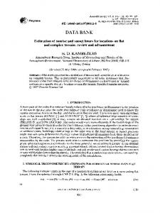
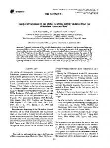
coefficients' dispersion We have seen that the SGLDM allows the creation of a new representation of the matrix (B type) and leads to the same interpretation for the two types of video and HF images [paragraph 2.3 and Fig. 2(b) and 2(d)]. The existing measures have not been defined for this type of representation of the matrix and consequently are not efficient. Thus, the ACM applied on a matrix similar to Fig. 2(a) will give, as the threshold value, the highest intensity of the last non-null coefficient Cij of the matrix, i.e. in the example of Fig. 2(a), a threshold equal to a. Indeed in the last non-empty block of the matrix (here B3 [a]) the contrast associated with the coefficient C0a reaches a maximum. Thus, we are trying to define measures that would be adapted to this type of matrix in order to evaluate the new possibilities provided by this approach. Our idea is to consider the coefficients present in the block B3 as a set of points balanced by the value of the coefficient Cij. These points belong to two categories: the points or coefficients relative to the background of the image, and the points relative to the transitions. Figure 3 provides a simplified representation of the problem on both types of images [Fig. 3(a) and 3(c)]. It shows three possibilities of matrix division, depending on the tested value for the threshold (cases 1, 2 or 3 in Fig. 3). Where the threshold corresponds to the high intensities (case 1) the block contains a set of coefficients, relative to the transitions, very little dispersed from the barycentre or the principal axis of inertia of the cloud. This dispersion will be all the fainter as the threshold is higher; on the contrary, when the threshold corresponds to a value that is close to the background of the image (case 2), the block contains a part of the cloud of points close to the mean value of the image. This compact cloud having a very strong relative impact, the dispersion around the common barycentre will then be faint. When the threshold is at
G. CORNELOUP et al.
286
(2X3)(1)
~i[t]
(1) (3)(p)2 (3) (1)
i
~"
/~j[tl
[ l'[
!
I
I
.J
I
/
)
J measure[t]
J
c)
a)
measure[t] ii~threshold (2) (3)
~threshold
(1)
(1)
(3) p (3) (2)
b)
(1)
d)
coefficients relative to background
I
]coefficients relative to transitions
Fig. 3. Analysis of the coefficient dispersion in a matrix. (a) and (b) Study of image l(a), (c) and (d) study of image l(d).
the boundary of this compact cloud, the dispersion will be maximum and will give a relative threshold value (case 3). The description perfectly follows the evolution of the signal/noise ratio (SNR). If the SNR deteriorates, the central cloud will expand and the threshold will intrinsically be higher. The expected evolution from a measure of the dispersion on this type of matrix is then provided in Fig. 3(b) and 3(d). In a previous study we used the Average Product of Variance Measure (APVM) ~4) as an indicator of the dispersion of the coefficients. This measure calculates the product of the square of the distances on both axes of inertia of the coefficients' cloud. These axes are provided by the mean values/~i and #j of these coefficients in the block B3. The description also corresponds to the product of the variances of the indexes i a n d j that are balanced in the block B3. B'[t] is the denominator that provides the sum of the coefficients of the block B3[t]. It allows to define the mean values #i a n d / i f
and K-1
t
(6)
and the APVM is given by: gK--1
t
~0 (i-"i[t])2Ci)
APVM[t] = ( 2
I
i=t j
i=t j
(7)
The mean values kti and #j depend on the value of t; in order to be able to use a recurrent definition of the measure we must re-write the expression (7) to eliminate the products between indexes and mean values. The expression of the APVM that lends itself to the recurrent calculation is given by: APVM[t] =
~ i=t
X
j=0 Z i=t
i2Ci/B'[t]-~i[t]
j=O
j.2 G/B , [t] - ~j[t] .
(8)
We also present another expression of the coefficients' dispersion that is less related to the flattening of the cloud of points around the central axis of inertia. The question is to measure the distance to the G barycentre in block 3 more simply. We shall
BSCAN image segmentation
287 A
define this measure Square of Mean Distance to the Center of Gravity Measure as follows (abbreviation
DMB): DMB[-t] =
[-(i-#i[t]) 2 + ( j - # j [ t ] ) z C i j \
vl ~Z
A d31 w ........L . . . . . . . . . i
i=t
j=0
B'[-t].
(9)
As for the A P V M the basic definition has to be modified to allow the recursive calculation, i.e.
d3 ZI1
,
Fig. 5. Dead zones in an image in accordance with vector d.
DMB[t]
\
i=t
3.1. Choosing vector d to obtain an A-type matrix
j=0
(10) 3. CHOOSING VECTORd There are m a n y possibilities to obtain a cooccurrence matrix according to vector d with the S G L D M . In this paper we present an application-specific approach to select rapidly or automatically a vector d according to the type of searched for analysis, i.e. whether we wish to use an A-type matrix and accordingly a measure of the ACM type, or prefer an analysis on a B-type matrix (background objects transitions) as well as a dispersion measure.
For a classical (video) image, a modulus r, much shorter than the m i n i m u m dimension of the object in the considered direction, is required. For an H F image the displacement of objects in the block B3 has to be prevented, which means preventing the connection between two pixels with opposite sign amplitudes [-Fig. l(e) case of the vector d2]. To avoid this displacement completely, the solution would consist of choosing the angle 0 = fl [-Fig. l(a)] as the analysis angle, then, to obtain an A-type matrix representing the objects, we should select a modulus that is largely smaller than dim~-nin(fl). 3.2. Choosing the vector d to obtain a B-type matrix
! 2 %
3
3.2.1. Definition of the characterization graphs. The point here is to build a B-type matrix, without object pairs, while limiting the interactions. According to the 0 observatio~a angle, and to avoid object pairs, a long enough vector d must be chosen. On the other hand, to avoid the relations between the objects, vector d must be shorter than the m i n i m u m distance between the objects; another solution lies in having a vector d that
a)
Research of preferential angle (characterization curve with angle)
step 1
Caracterisation
]
I
Research of vector d modulus [ ( characterization curve with distance )
step 2
1
2
3
4
5
step 3
I
I
Measure calculation
I
Segmentation
]
b) Fig. 4. Analysis of a characterization curve with a dispersion measure. (a) HF image with two objects and five vectors d and (b) characterization curve.
step 4
Fig. 6. General algorithm.
288
G. CORNELOUP et al.
>
scanning axis
a)
crack top crack bottom
weld corner
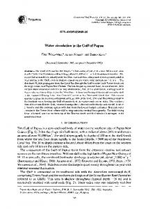
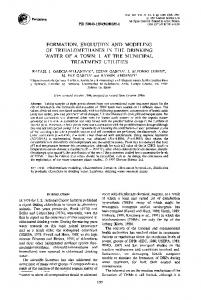
-128[~1+127 b) Fig. 7. Acquisition of a BSCAN image. (a) Ultrasonic testing of a weld by the immersion technique and (b) resulting image (421 signals of 1018 points).
would be longer than the m a x i m u m distance between the objects. As these conditions are not always wellknown a priori, specific analysis has to be made to respond to this problem. The idea, developed by several authors such as Zucker~l 3) or Harlow, Trivedi and Conners ~11,14) consists of evaluating several matrices and defining a rule to determine the optimal matrix a m o n g the matrices that have been calculated. The optimization depends on the formulated problem. To evaluate these matrices
it is in particular possible to calculate the evolution of a parameter or a measure defined from the coefficients C~j; the extrema that are obtained give the optimal value or values. We call characterization graphs the functions that make this analysis possible. As we have to select a threshold, we also have to integrate the threshold value in the analysis function of the matrix behaviour. We keep the measures to obtain this relation with the threshold values. O n the whole we may define the measure characterization graph for
BSCAN image segmentation the definition of a threshold (abbreviation GCMDS) by: GCMxDS[r, 0] = optimum [Measure(r,0)]. (11) r,OES
~ = 0 ,K -
1
Equation (11) reveals that it requires many calculations of matrices depending on the domain S where r and 0 are defined. This type of approach is thus difficult to exploit. In our study we had two possibilities to define the Measure(r, 0): the APVM and the DMB measure (cf. Section 2.5). We have seen that the problem to create a B-type matrix does not depend on the angle 0 as the analysis is similar whatever the angle, the sole dimensions of the objects vary according to the angle. Therefore, their is no real necessity for optimization according to the angle. The angle of analysis is set for/~-~/2 from the experience acquired on this type of image because it allows us to obtain configurations more easily in which the vector d is greater than the maximum distance between the objects. We can thus obtain, by increasing the value of the modulus r, all the possibilities of specific connections from the pixels of an object: within the same objects, between objects, then only between the object and the background of the image. Thus, the problem here is restricted to a characterization curve according to the modulus r. 3.2.2. Analysis of the characterization curves. To evaluate the expected behaviour of the characterization curves using the APVM and the DMB measure on B-type matrices, let us consider a pattern of the image with two neighbouring objects [Fig. 4(a)]. As both measures ~re defined as dispersion measures, it is
a)
289
the maximum dispersion value calculated for the matrices that proves of interest as discriminating parameter. The behavior of the characterization curve is displayed in Fig. 4(b). The first part of the curve concerns the lower values of the vector d; the matrix coefficients are distributed along the diagonal; consequently the dispersion is very faint and it is null when r equals zero. Then when the vector d connects the pixels with opposite sign amplitudes, the objects are displaced in the zone of the blocks B3, the matrix nearly completes a 90 ° rotation and the dispersion measured in the blocks B3 is at its maximum. Then the maximum of the measure decreases until the modulus r allows the connection of the objects; then again more coefficients outside the diagonal are created. If the maximum amplitudes of the objects are different, the measure cannot reach its maximum again as the pairs obtained cannot re-create the differences in amplitude of the object having the maximum amplitude. The curve raises to a local maximum. Finally, when the modulus r is superior to the maximum distance between two objects, i.e. longer than the zone of the image containing the defects, only coefficients of the background-objects-type are created. A B-type matrix is obtained, the general aspect of which does not evolve any more: all the pixels of the objects are connected to the noise pixels. Therefore the maximum of the measure is steady (case no. 5 in Fig. 4). For the high values of the modulus, the problem of boundary effects arises. The image really uses changes and may modify the stability of the characterization curve described above. Indeed the definition of the cooccurrence matrix according to the SGLDM creates
b)
Fig. 8. Two images of weld testing. (a) Image containing a 7 mm crack (425 signals of 1018 points) and (b) image of five cracks with a transducer movement parallel to the defect (389 signals of 1018 points).
290
G. C O R N E L O U P - 128
amplitude i
et aI.
+ 127
-12[
a m
P 1 i t
a
ae J
~ f
+127
a) matrix
b) image
amp
. j
b) measure
c) image
5
38
c) measure ~56.
9'
i
itu.e
d) measure
i
• d) image
Fig. 9. Results for A C M m e t h o d . (a) M a t r i x o b t a i n e d from i m a g e 8(a) ( m o d u l u s r = 1, angle 0 = - 9 0 ° ) , (b) curve of m e a s u r e A C M for i m a g e 8(a) ( m o d u l u s r = 1, angle 0 = - 90 °) a n d t h r e s h o l d e d i m a g e (thresholds: 43 a n d 208), (c) curve of A C M m e a s u r e for i m a g e 7(b) ( m o d u l u s r = 1, angle 0 = - 90 °) a n d t h r e s h o l d e d i m a g e (thresholds: 64 a n d 210) a n d (d) curve of A C M m e a s u r e for i m a g e 8(b) ( m o d u l u s r = 1, angle 0 = - 9 0 °) a n d t h r e s h o l d e d i m a g e (thresholds: 38 a n d 185).
BSCAN image segmentation
on the image two dead zones ( Z l l and Z12) that will never be visible through the analysis (Fig. 5). These zones are positioned in the corners of the image, they are null if vector d is vertical or horizontal. Additionally, the coordinates dx and dy of vector d are limited to half the image's dimensions, i.e. M/2 and N/2, respectively. Beyond, the central zone of the image is no longer taken into account in the matrix: respectively, it is a vertical zone (ZV) if the vector is horizontal (d3) and it is a horizontal zone if the vector is vertical (d2) (Fig. 5). In our type of image of a weld tested by ultrasound (Figs 1 and 7), the dead zones do not pose any major problems, yet the problem is not altogether solved for other types of images. F r o m the characterization curves described above two possibilities arise to select the modulus r. We first selected the global minimum of the characterization
0.00
291
curve situated behind its maximum. Secondly we considered a local minimum corresponding to the case when a vector with a short dimension is longer than the minimum dimension of the objects, but is short enough not to establish a connection between the objects. The drawback is that a local minimum does not guarantee that an ideal situation of that type has been found. The first solution is so to be chosen even if it requires more calculations.
4. GENERAL ALGORITHM Figure 6 shows the global process-of how to obtain a thresholded image. The first phase that consists of defining the optimal orientation is kept, so that the general description may be represented.
0.00
~M.~, modulus r
19~
modulus
r
199
modulus
r
149
a) DMB
a) APVM
0.00 0
modulus r
149
b) APVM
b) DMB
i.le+~S
~.~
0.00 modulus r
O
c) APVM
255
modulus r
c) DMB
Fig. 10. Characterization curves according to the modulus r. (a) Curves obtained from image 8(a), (b) curves obtained from image 7(b) and (c) curves obtained from image 8(b).
255
292
G. CORNELOUP et al.
5.
IMPLEMENTATION
AND
DISCUSSION
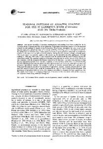
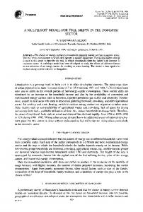
5.1. Building the image The diagram in Fig. 7 summarizes the acquisition process for ultrasonic images. The figure displays the control of a crack in a weld. The transducer operates in the emitter-receiver mode with a control angle ~ and moves perpendicularly to the defect. The signals obtained for each position of the transducer are then juxtaposed to create an image known as a BSCAN image, whose horizontal axis is a spatial axis and whose vertical axis is a temporal axis. Figure 7(b) gives the built image and its scale of colours. We have shown our results on test images, which are characteristic of the problem of crack detection in welds. Two other images are represented in Fig. 8. The first is the image of a crack (cross-view) in a block of steel (as Fig. 7); it is t h e image which is easiest to segment as the signal-to-noise ratio is very high. The third image displays five cracks examined with a transducer movement parallel to the defect. We have seen that two types of analyses may be developed according to the type of matrix that is built. Different measures to obtain threshold values were used. We shall now compare the two analyses.
avoid a subjective choice of vector d when building a B-type matrix (background transitions). Figure 10 represents the characterization curves for the three images and the two A P V M and D M B measures. The behaviour of the curves corresponds to the description in Section 3.2.2. For each of these images, when vector d is long enough, only the pairs of pixels of the background object or background background type are built. It is easy to select a value for vector d following the position of the m a x i m u m of the characterization curve that corresponds to the maximum of the internal
-
128
amplitude i
+ 127
-128
a m
p t U
d e
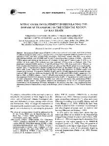
5.2. A-type matrices and A C M measure In the process of building an A-type matrix without having any internal interactions, we are significantly limited in the choice of vector d, because of the intrinsic form of H F signals. Indeed there is a temporal shifting between two signals that is created by the difference of the ultrasound's path (two different positions of the transducer); thus if dx is different from 0, this may create connections between amplitudes with opposite signs, i.e. internal interactions. Also, depending on the sampling rate, if dy is greater than 1, there may be internal interactions when the slope of the signal is very steep. With H F signals very close pixels can have very different amplitudes. An A-type matrix is thus obained with a very short vector d. For the analysis of the three images by an A-type matrix (Fig. 7 and 8) we used the following vector ( d x = 0 , dy= 1). Figure 9 provides the three thresholding curves and the segmented image. It also represents an A-type matrix obtained on an H F image. To obtain a representation in the form of an image of all the matrix coefficients, we have chosen a logarithmic scale. The results obtained on these three images show that the ACM measure does not properly fit this type of image as it gives thresholds that are too high and important echos only are thresholded.
J
• >.,. " '
: .: ~' . ~ :
~"
i
."
• ~~'
"
.
+127
a) amplitude i
-128
+127
-128
m
p !
I e
,
,
l
+127 5.3. B-type matrices and dispersion measures 5.3.1. Characterization curves. We have previously shown that a characterization curve was necessary to
b) Fig. 11. Characteristics of two matrices. (a) Matrix obtained from image 8(a) (r = 3, 0 = - 6 0 °) and (b) matrix obtained from image 8(a) (r = 108, 0 = - 60~).
BSCAN image segmentation
293
J amplitude
255
a) measure a) image
4e÷04
~,
amplitude
23~
b) measure b) image 1.2e*03
9
amplitude
240
c) measure
c)matfix Fig. 12. Results for the APVM method. (a) Curve of APVM measure for image 8(a) (modulus r = 1, angle 0 = - 9 0 °) and thresholded image (thresholds: 110 and 155), (b) curve of APVM measure for image 7(b) (modulus r = 1, angle 0 = 90°) and thresholded image (thresholds: 104 and 151), (c) curve of APVM measure for image 8(b) (modulus r = 1, angle 0 = - 9 0 °) and thresholded image (thresholds: 129 and 131).
294
G. C O R N E L O U P et al.
J
0
amplitude
255
a) measure a) image
.2e+03
amplitude
23~
b) measure b) image
amplitude
24C
c) measure
c) image Fig. 13. Results for the D M B method. (a) Curve of D M B measure for image 8(a) (modulus r = 1, angle 0 = - 9 0 °) and thresholded image (thresholds: 102 and 159), (b) curve of D M B measure for image 7(b) (modulus r = 1, angle 0 = - 90 °) and thresholded image (thresholds: 96 and 158), (c) curve of D M B measure for image 8(b) (modulus r = 1, angle 0 = - 9 0 °) and thresholded image (thresholds: 105 and 156).
BSCAN image segmentation interactions (the matrix is then established according to the second diagonal). The various secondary peaks correspond to interactions between objects. To a certain extent, the characterization curve can be compared with an inter-correlation function as it reaches successive maximum when two objects are linked by vector d. The choice of vector d is very reliable in the flat part of the characterization curves: the values of the thresholds and the behaviour of the matrix scarcely evolve. Figure 11 shows two matrices: one matrix is obtained at the maximum of the characterization curve, and the other is obtained for a vector d chosen in the flat zone of the characterization curve. This figure illustrates how very different these two matrices are and how rich the analysis of the cooccurrence matrix based on the SGLDM method is. 5.3.2. Threshold images. Figures 12 and 13 show the thresholding curves and the segmented image for the APVM and DMB curves. All the really important echos are subjected to thresholding, which will then allow an analysis of their relative positions in order to size up the defects and characterize the mechanical behaviour of the weld. The results are largely superior to the results obtained through an analysis using a classical matrix of the background object type (paragraph 5.2); they confirm that for this type of image a really innovative approach was essential. In most cases, both measures give very similar results. The calculations of the block B3 coefficients' dispersion as an indicator of the end of the homogeneous distribution of the coefficients relative to the image background seem to be reliable. Indeed the same idea expressed differently provides almost identical results. The APVM measure seems to be more sensitive as it detects fainter echos. Yet its expression (7), which, in a simplified way, corresponds to the product of the width by the length of the branches of the matrix, is revealed to be at fault on the third image. The proposed thresholds [Fig. 12(c)] are much too low. The DMB measure has therefore to be selected as the most pertinent solution. The complete approach defined in Section 4 thus allows very good thresholding results on these ultrasonic BSCAN images. We have established that the BSCAN images can be correctly analysed with our method on the condition that the signal not be saturated, which would distort the distribution of the coefficients in the matrix. This means that the surface echo should be eliminated if it were very strong (i.e. saturated). The obtained thresholds prove satisfactory to the control qperators, the method can be totally automated and allows us to consider the processing of important values of data. The calculation times depend on the number of matrices that are necessary to calculate the characterization curve and define the appropriate vector d. The mean time on an HP 715-33 workstation is about a few minutes. It is thus possible to control welds more systematically and accordingly improve the reliability of the controled systems.
295 6. CONCLUSIONS
This global analysis of a new approach to the use of the cooccurrence matrix for a thresholding problem leads to drawing several conclusions. We have seen to which extent the extension of the SGLDM approach, that allowed us to obtain spatial relations between pixels which are far from each other, may be used to obtain adequate information but different from the standard approah by cooccurrence. This proposed approach is different from the standard one which is more oriented towards the micostructures of the image. We are threfore seeking more global relations between macrostructures; objects and image background. We rather analyse the boundaries between objects and image background. We have developed a method aimed at automatically choosing the dimension of vector d, which often is the stumbling block of an approach based on the SGLDM method. There is a great number of possibilities to choose the vector. There are two parameters to set: the modulus of vector d and its angle. In the present study the angle is linked to the preferential orientation of the image caused by the propagation of ultrasounds. The necessity for selecting the modulus which depends on the properties of the image (or rather on the distribution of objects on that image) led to the definition of characterization graphs. This notion would be applicable if the choice of the angles were to be considered in the same way. We would then have twodimensional characterization graphs. On the other hand, the number of calculations required would be a handicap. Let us note that the drawback of the method is to create image zones which are not studied. For other images one would have to reconsider the problem in selecting a second vector whose angle would be of the opposite sign. The proposed measures to calculate the thresholds offer the advantages of being efficient and reliable for the two types of images (video and HF). These measures therefore have a very interesting and global character. The analysis also allows to obtain two different thresholds, on either side of the mean value; in the case of H F images, the two thresholds account for the asymmetry of the ultrasonic signals. Our results on real test images are very satisfactory for the DMB measure, which better account for the dispersion of the coefficients in the B3 block than the APVM measure whose definition was at fault about one example. The global analysis implementation matrices with particular shapes and characterization and thresholding curves whose general aspects are very similar. Thus, in the case of a purely, automated approach with a very large volume of processing without observations by the operator, it will be possible to define shape parameters for these matrices or curves. Whether or not the current analysis is still valid will be known via these parameters. This would make the problem images possible to detect: for example, images in which the signal is saturated.
296
G. CORNELOUP et al.
To place the study in its N D T context, let us recall t h a t for any a u t o m a t i c thresholding method, the suggested m e t h o d s h o u l d be coupled with a defect detection method. The p r o b l e m is to avoid the false alarms created by the systematic calculation of a t h r e s h o l d even if the image does n o t c o n t a i n any defect. This p r o b l e m concerns the defintion of the specifications of the control system t h a t should indicate the time w h e n the a u t o m a t i c analysis of the picture occurs. At last, the t h r e s h o l d a n d segmented echos can be m a n i p u l a t e d by an expert system that will identify and classify the defects. To conclude o n the possible developments of the present study let us note that the m e t h o d s for the acquisition of ultrasonic images allow us to have a volu m e of data available (several BSCANs); we shall consider in a very b r o a d perspective the use of cooecurrence matrices in a 3D volume in order to have a third axis available for defect identification.
5. 6. 7. 8. 9. 10. 11. 12.
REFERENCES
1. P. Benoist, F. Cartier, G. Pincemaille and J. Clicques, Syst6me pour l'acquisition, la recherche, le traitement et l'analyse des ultrasons (Spartacus), in Acres du let Congr~s COFREND sur les essais non destructifs, pp. 365-369, Nice (1990). 2. G.P. Singh and S. Udpa, The role of digital signal processing in NDT, N D T Int. 19, 125 132 (1986). 3. J. Moysan, G. Corneloup, I. E. Magnin, P. Benoist and N. Chapuis, D6tection et dimensionnement de d6fauts en imagerie ultrasonore, in Proc. du X I l l Ome Colloque sur le Traitement du Signal et des Images, pp. 181 184. JuanLes-Pins, GRETSI, (1991). 4. J. Moysan, G. Corneloup, I. E. Magnin and P. Benoist, Matrice de cooccurrence optimale pour la segmentation
13. 14. 15.
16. 17.
automatuque d'images ultrasonores, Traitement Signal 9, 309-323 (1992). R. M. Haralick and L. G. Shapiro, Image segmentation techniques, Comput. Vis. Graphics Image Process. 29, 100 132 (1985). R. M. Haralick, K. Shanmugan and I. Deinstein, Textural features for image classification, IEEE Trans. Systems, Man Cybnet. 3, 610-621 (1973). R. M. Haralick, Statistical and structural approaches to texture, Proc. IEEE 67, 786-804 (1979). J.S. Weszka and A. Rosenfeld, Threshold evaluation techniques, IEEE Trans. Systems Man Cybernet. 8, 622629 (1978). B. Chanda and B. B. Chaudhuri, On image enhancement and threshold selection using the gray level cooccurrence matrix, Pattern Recognition Lett. 3, 243 251 (1985). B. Chanda and D. D. Majumber, A note on the use of the gray level cooccurrence matrix in threshold selecction, Sig. Process. 15, 149-167 (1988). S. K. Pal and N. R. Pal, Segmentation using contrast and homogeneity measures, Pattern Recognition Lett. 5, 293304 (1987). R.W. Conners and C.A. Haralow, A theoretical comparison of texture algorithms, IEEE Trans. Pattern Analy. Mach. Intell. 2, 204 222 (1980). M. M. Trivedi, C. A. Harlow, R. W. Conners and S. Gob, Object detection based on gray level cooccurrence, Computer Vis. GraphicsImage Recognition28,199 219(1984). C. A. Harlow, M. M. Trivedi and R. W. Conners, Use of texture operators in segmentation, Opt. Eng. 25, 1200 1206 (1986). M. Neveu, A. Dipanda, D. Plantamp and H. Diebold, Segmentation d'images 6chocardiographiques par analyse de texture, Innov. Tech. Biol. Med. 10, 413-428 (1989). D.C. Tseng and W.S. Shieh, Plume extraction using enthropic thresholding and region growing, Pattern Recognition 56, 805-817 (1993). J. F. Haddon and J. F. Boyce, Image segmentation by unifying region and boundary information, IEEE Trans. Pattern Anal. Mach. Intell. 12, 929-948 (1990).
About the Author--GILLES CORNELOUP is the director of the LCND and a sejaior lecturer at the IUT in
Aix en Provence. He received a Ph.D. degree in 1988 for a study on the numerical processing of ultrasonic images and its applications to the detection of faults. His main research concerns signal and image processing with a view to the characterization of austenitic and heterogeneous materials. He is member of the GDR 134 TDSI team of the CNRS.
JOSEPH MOYSAN is a senior lecturer at the IUT in Aix en Provence. He received a Ph.D. degree from the National Institute of Applied Sciences of LYON (INSA) in 1992. His research interests include image processing applied to Ultrasonics and Non Destructive Testing, more particularly, the analysis of images and their segmentation that uses cooccurrence matrices. He is member of the GDR 134 TDSI team of the CNRS. About the Author
About the Author--ISABELLE E. MAGNIN has been a researcher with the National Institute for Health and Medical Research (INSERM) since 1982; she heads a team of researchers involved in the treatment of 3D images and 3D dynamics. She is an expert in medical imagery. She is an active member of the GDR 134 TDSI team of the CNRS. She is also a member of IEEE and EURASIP.